


Abstract
The COVID-19 pandemic has emphasized the need to consider multiple and often novel perspectives on contemporary policymaking in the context of technically complex, ambiguous, and large-scale crises. In this article, we focus on exploring a territory that remains relatively unchartered on a large scale, namely the relationship between economic inequalities and excess mortality during the COVID-19 pandemic, using a dataset of 25 European countries spanning 300 regions. Our findings reveal two pathways by which economic asymmetries and inequalities can observably influence excess mortality: labor market structures (capturing concentrations of industrial jobs) and income inequalities (capturing concentrations and asymmetries in income distribution). We leverage our findings to offer recommendations for policymakers toward a more deliberate consideration of the multidimensionality of technically complex, large-scale crises with a high degree of societal embeddedness. These findings also urge future scholarship to utilize a range of parameters and indicators for better understanding the relationship between cues and outcomes in such complex settings.
In hard-hitting, society-wide crises, critical policy responses have significant implications for lives and livelihoods. This makes elucidating the design underpinnings and key dynamics influencing crisis responses and their outcomes central and pressing concerns for governments worldwide (Dunlop et al., 2020; Weible et al., 2020). Throughout the COVID-19 crisis, there was somewhat of a global consensus on the broad lines of action. Since the beginning of the pandemic and even until the time of writing this article (as the fifth wave of infections struck), COVID-19 policy responses continue to rely on non-pharmaceutical interventions (NPIs; such as physical distancing, updated hygiene standards, working from home, etc.) as highly effective and key tools in the fight against the pandemic (Li et al., 2020). Naturally, such interventions are societally embedded and behaviorally moderated, hence they largely depend not only on the willingness of citizens but also on their ability and capacity to comply and cooperate (e.g., Cao et al., 2020; Hartley & Jarvis, 2020). This further emphasizes the established need for considering how policies interact with societal contexts (Weible, 2018; Zaki et al., 2022), particularly in such large-scale crises where the policy-society dynamic becomes even more entwined and as the crisis transcends sectorial and societal boundaries (Zaki & George, 2021). Within these settings, policymakers need to consider competing and even conflicting contextual factors and logics that can influence response strategies, policy fit and effectiveness (see Maor & Howlett, 2020; Zaki & Wayenberg, 2021). In addition to systemic and structural factors such as capacities, politics, governance settings, and policy legacies (e.g., Béland & Marier, 2020; Capano et al., 2020; Lee et al., 2020; Migone, 2020), policymakers also need to consider societal factors that potentially influence both citizens’ willingness and ability to comply to pandemic policies.
As a compelling aspect of such systemic and societal contexts, the concept of inequalities has been central across various fields of study, from social studies (e.g., Walker & Burningham, 2011) to development studies (e.g., Johnson & Wilson, 2000), and public health (e.g., Siu, 2020; Szreter & Woolcock, 2004). Due to their growing and far-reaching implications, research on various social inequalities has found a relatively nascent foothold in public policy research, particularly focusing on policy designs. This effort has largely focused on exploring the implications of inequalities for certain demographic groups within specific societies, and thus for ensuing policymaking (e.g., Fusaro, 2020; Huber et al., 2020; Plomien, 2019). However, public policy literature still relatively lags in exploring tangible society-wide implications of inequalities and their influence on policy outcomes, particularly in large-scale crises. Accordingly, burgeoning COVID-19 public administration literature recently began exploring how inequalities can disproportionately influence (particularly via restricting) the ability of certain groups to safely maneuver the pandemic. This remarkable (and needed) effort was focused on two distinct yet related streams, first: structural capacity and systemic disparities such as urban development and access to healthcare (e.g., Deslatte et al., 2020; Martin-Howard, 2020), second: social disparities such as those based on income, gender, race, and occupation (e.g., Beland et al., 2020; Chan, 2020; Lynch, 2020). A majority of the said literature adopts single case designs focused on assessing how the pandemic disproportionately affects certain demographic groups, thus endeavoring to partially alleviate some of their burdens of inequality (e.g., Gy et al., 2020). While this has illuminated our understanding of how inequalities play out during crises, we are still to see concerted large-scale analyses to explore how certain disparities impact key pandemic policy outcomes, while particularly looking at the ensuing implications for policymaking both inter- and intra-crisis and going beyond a limited set of directly impacted demographics using robust comparable indicators within different regions.
In this article, we push forward the understanding of the relationship between public policy and economic inequality by exploring how economic disparities could be contributing to excess mortality during the COVID-19 pandemic. We do so by constructing a panel model with observations from 25 European countries spanning 300 regions for 52 weeks starting January 2020. In constructing this model, we account for varying contextual configurations such as policy response stringency, population parameters, and healthcare capacity among several others. Here, we leverage the simultaneous occurrence of a policy crisis across multiple jurisdictions to draw critical lessons through exploring and comparing diverse responses and performance indicators. We then employ our findings to highlight how can practitioners strengthen crisis policy designs in similar future crises in light of the explored relationships.
By pursuing these inquiries, our contribution is threefold. Theoretically, we capitalize on state-of-the-art emerging data to extend our understanding of crisis policymaking and policy outcomes by exploring largely unchartered relationships between economic inequality and mortality within different contextual configurations. Empirically, we provide a novel account of how economic disparities can influence policy outcomes in society-wide crises and offer a host of explanatory parameters that helps highlight this relationship and its implications. We also advance the public policy research agenda on inequalities by repositioning the issue beyond directly impacted groups into a society-wide issue with tangible implications on the overall regional and national levels. Practically, we offer key insights for policymakers to guide future policy design across varying contexts. In doing so, we respond to the call for practical, and relevant research on COVID-19 in public administration scholarship while presenting a theoretical contribution of novelty and utility (Corley & Gioia, 2011; Dunlop et al., 2020).
This article is organized as follows: In Inequalities and pandemic policy outcomes, we construct our theoretical framework by plotting pathways between economic disparities and pandemic policy outcomes, in Methods we elaborate on the methodological framework and data used, we offer our results in Results, followed by a discussion of results, recommendations, and general conclusions in Discussion and implications.
Inequalities and pandemic policy outcomes
As previously established, there are both theoretical and empirical indications as to the far-reaching implications of inequalities. Such implications can be exacerbated in crises, particularly within the context of a global pandemic. Yet, what is inequality within this context? Binelli et al. (2015) articulate “social inequality” as a multidimensional concept that expresses a manifold of disparities within a society (e.g., wealth and income, gender, education, and housing among several others). This motivates an inquiry into what particular strand of disparity can significantly influence pandemic policy outcomes, yet can be reliably measured, and compared across various contexts? We suggest that answering this question should consider three main parameters: First, the relevance and potential influence on key entailments of pandemic policy responses. Second, the availability of robust measurements. Third, a consideration of measurement equivalence to enable cross-context comparisons (George et al., 2020). We begin by highlighting how economic inequality provides relevant and plausible theoretical pathways to influence COVID-19 policy response effectiveness.
Economic disparities and potential implications for COVID-19
Social inequalities are multidimensional (e.g., economic, gender-based, race-based, etc.). Different dimensions of inequality tend to “move together”, thus can progressively amplify and reinforce each other, particularly as they can be closely entwined within the social context (Binelli et al., 2015). Here, we postulate that economic inequality is well-positioned to meet the three above-mentioned criteria of relevance to pandemic policies, availability of robust measurements, and measurement equivalence.
In terms of relevance, entailments of COVID-19 policy responses focused on NPIs, access to healthcare, and general health are demonstrably influenced (even often shaped) by economic inequality. Economic inequality (manifested in income disparities for example) can induce implications in key areas pivotal for pandemic policy responses and their outcomes. This includes access to basic sanitation (e.g., Satur & Lindsay, 2020), access to parks and open spaces, which enhances population health and provides means for physical distancing (e.g., Sugiyama et al., 2018; Wüstemann et al., 2017; Xiao et al., 2019), disproportionate pollution burden (e.g., Gilderbloom et al., 2020), and urban density (e.g., Arundel & Hochstenbach, 2019). This is in addition to the established relationship between economic inequalities and access to healthcare (Bambra et al., 2020), increased mortality, and reduced life expectancies (Kawachi et al., 1997; Szreter & Woolcock, 2004). Recent research has also shown a significant association between socioeconomic inequality and several comorbidities that also align with those of COVID-19 such as obesity, cardiovascular diseases, asthma, diabetes, oncological complications, and arthritis among several others (e.g., Carrilero et al., 2020; Hosseinpoor et al., 2012; Khanolkara & Patalay, 2020; Mackenbach et al., 2000; Patel et al., 2020). As such, economic inequality can be considered a robust indicator of susceptibility to COVID-19 induced mortality.
Furthermore, research within the COVID-19 context has recently started pointing out the potential relationship between economic disparities and the nature of labor market structures on one hand, and the ability of citizens to comply to stay at home orders on the other. In some contexts, this was viewed to be due to factors pertinent to urban and dwelling issues (Chan, 2020) or work-type arrangements (Bonacini et al., 2020; Gallacher & Hossain, 2020). Second, economic inequality and labor market structures are established concepts; thus; robust and reliable measurements exist and are widely used, including measures such as income quintile ratios, people at risk of poverty, Gini coefficients, or employment sector statistics (e.g., Drezner et al., 2014; Hatch & Rigby, 2015; Zimm & Nakicenovic, 2020). Third, as established measures, economic inequalities and labor market structures avail standardized benchmarks suited for- and used in- cross-country comparisons. Put together, these logics position economic inequality as a robust independent variable underpinning pandemic policy outcomes across various contexts.
In sum, existing literature positions economic inequalities and labor market structures as societal sources of accrued individual exposure to key factors that influence the pandemic’s outcomes. Thus, studying economic inequalities as key parameters for understanding the evolutions and outcomes of the pandemic becomes essential. This is especially when individual panel data remain relatively scarce, neither necessarily representative of the population nor indicative of individual-level societal positioning.
Even though literature suggests the existence of a potential, general relationship between economic disparities and disproportionate effects of the pandemic, relatively little is known about the nature or key parameters shaping it. To address this, we focus on two underlying parameters or pathways through which economic inequality can impact the state of the pandemic: the labor market structure and the distribution of income. These two parameters do not necessarily capture the same underlying notions: income distribution, on its own, is a measure of inequality. However, the labor market structure (e.g., the proportion of the labor force working in the industrial and manufacturing sector)—while not necessarily identical to income inequality—models a different type of economic asymmetry, not based on an individual’s or household income but on someone’s profession. This relationship could mean that the pandemic exerts disproportionate burdens on some professions, for instance, disproportionately impacting industrial workers whose jobs cannot be easily automated or conducted remotely, particularly with the growing precariousness of industrial jobs (e.g., Kalleberg, 2012). This would then crystallize existing tensions and generate further distributional effects as the pandemic’s toll is disproportionately incurred by different groups.
In the following analysis, we take a closer look at two specific pathways by which economic inequality can influence excess mortality as one of the pandemic’s key outcomes. The first pathway is mediated through the labor market configuration. We posit that workers in the industrial sector (excluding services) are usually employed in jobs that cannot be easily (if at all) remotely conducted. Thus, a significant share of these workers will have to continue to work in situ despite potentially worsening health conditions. While indeed some of these manufacturing plants could have been temporarily closed at the onset of the pandemic, they were fast to resume work once initial restrictions were lifted. As such, workers in such sectors (whose employment was not terminated and were allowed to return to work), were not necessarily eligible for unemployment subsidies or furloughing schemes should they decide not to return to their jobs. Subsequently, workers in these sectors were more likely to face a fundamental trade-off between economic and health security, than their nonindustry counterparts. As such, industry employees can be expected to face higher infection and mortality risks (For initial indicators, see for example, Arceo-Gomez et al., 2021; Milligan et al., 2021; Sepulveda & Brooker, 2021). Accordingly, areas with higher shares of employment engaged in these industrial activities can be expected to be relatively more affected by the pandemic than areas where employment is less dependent on such activities. Emerging findings also indicate that individuals engaged in such sectors can be at a significantly higher risk of infection and mortality (e.g., Milligan et al., 2021). There are similar initial indicators to this mechanism in emerging COVID-19 public administration research, however not yet scaled up or further explored at this level of analysis (e.g., Chan, 2020).
The second pathway is focused on income concentration and inequality. When income concentration and inequality are high, several dynamics can exacerbate excess mortality. First, as we previously established, higher economic inequality is associated with relatively limited access to healthcare, smaller living spaces, overcrowding, relatively less access to sanitary resources, open spaces, and proneness to having more co-morbidities that aggravate the risk of severe COVID-19 complications (e.g., Carrilero et al., 2020; Hosseinpoor et al., 2012; Khanolkara & Patalay, 2020; Mackenbach et al., 2000; Patel et al., 2020).
Potential COVID-19-related excess mortality as a dependent variable
The COVID-19 crisis is multidimensional, with a large range of stakeholders. Hence, establishing normative or general views of success in such contexts and under complex conditions is challenging (see McConnell et al., 2020). Additionally, while such assessments require comparative perspectives, the crisis has underlined variations in data collection and measurement equivalence (George et al., 2020). As such, our main focus is on identifying robust and clear indicators that consider measurement equivalence and key common policy objectives. The choice of a dependent variable within this context is a delicate undertaking, particularly as several options exist, naturally, each with some advantages and drawbacks. A widely used variable is the number of infections. At first glance, this seems to be the best in being able to capture the spread of the pandemic. However, it suffers several issues, particularly with varying national capacities and reporting standards. This makes the variable not entirely suitable for large-scale cross-country comparisons. The same can be argued for the viral reproduction rate (commonly known as the R-value). Alternatively, COVID-19-induced fatalities can be considered. However, this also suffers from similar issues as the first two variables (infections and reproduction rate), particularly as what counts as “COVID-19”-related fatalities can significantly vary across different jurisdictions, either due to genuine capacity and standards variations or political decisions. Additionally, as nations can often change their reporting standards along the way, this potentially introduces inconsistencies in longitudinal analysis and complicates large-scale cross-comparisons (Zaki et al., 2022; George et al., 2020; Karlinsky & Kobak, 2021).
Several issues that complicate conducting robust cross-country comparisons can be significantly reduced if we are to accept a relatively limited loss of precision in the dependent variable measurement. Here, we argue for the utility of employing overall excess mortality as the dependent variable. Within this context, excess mortality, refers to a variable that captures the differential between the overall death rates in 2020, and those from previous years. This is while having the assumption that there are no other exogenous factors that could have contributed to significantly higher mortality throughout the period of observation. As such, this indicator can provide a somewhat comparable and acceptable estimate of the net mortality effects of the pandemic, at the cost of foregoing precision on the specific causes of death (which nevertheless remains a controversial issue). Accordingly, this provides an estimation of the net effect of mortality-related consequences, as such: fatalities caused by preexisting conditions and comorbidities, or depleted healthcare capacity are counted negatively, while the decrease in car accident fatalities (due to lockdown measures) would be counted positively. Hence, this measure provides only an overall estimate of the toll of the pandemic (Zaki et al., 2022). However, there is no doubt that for international comparisons, the type of bias introduced by relatively lower precision is preferable to biases due to different data generating processes. While the bias in precision is very likely to be similar across all countries, and therefore does not severely impair territorial comparisons, different recordings of what constitutes a COVID-19 fatality, or of what case incidence really measures, render cross-country comparisons far less reliable. Additionally, lending more substantiation to this variable selection, although different governments had variations in response philosophy, with some focusing on minimizing economic impact (thus mainly focusing on protecting the most vulnerable e.g., Lee et al., 2020; Pierre, 2020), and others taking harder approaches to suppress the overall community transmission (e.g., Capano, 2020); both response strategies entailed a focus on reducing mortality as a key policy outcome (Zaki et al., 2022).
Hence, given the need for temporal and geographical comparability, excess mortality is positioned as a theoretically plausible, empirically, and practically recognized dependent variable. As such, here, excess mortality is operationalized as the number of deaths that exceed what was observed under “normal conditions” as a baseline in previous years. We compute these scores as the weekly differential of mortality rates, per region, over the average for the same week for the past 10 years prior to the pandemic (In doing so, we go further beyond the statistical practice of only using baselines based on the previous 5 years). This use and operationalization of excess mortality have been robustly established and widely employed to capture pandemic-related casualties (see Achilleos et al., 2021; Chan et al., 2021; George et al., 2020; Karlinsky & Kobak, 2021). Utilizing excess mortality as our dependent variable allows us to also consider the indirect yet likely COVID-19-related fatalities (that could occur as a result of reduced healthcare capacity and decanting hospitals, medicine shortages, etc.), particularly in the absence of observable significant confounding mortality causes during within the period of analysis.
Methods
Level of analysis
To answer our central question, we leverage an econometric analysis of the relationship between inequality and excess mortality during the first year of the pandemic. Importantly, given the nature of economic inequality, differences within countries are often as important as differences between countries. Therefore, an exploration of the impact of economic inequality requires a regionalized dataset. Thus, whenever feasible, we conduct the analysis using regionally disaggregated data. This means that, in practice, we often cannot look at direct measures of economic inequality for all regions, particularly as only a subset of regions reports income inequality data. Furthermore, this also means that we cannot fully account for regional differentiations in the intensity of lockdowns (mainly as this data is not yet available). When viable, we conduct multilevel analysis at the NUTS2 regional level to account for policy differentiations at the country level, but this is nearly equivalent to introducing country fixed effects.1
Data
As discussed, our dependent variable is excess mortality, computed as weekly percentage deviations in mortality between 2020 and previous years. More in detail, for any given region in each week of the year, we compute the percentage increase in mortality over the average mortality of the same week of the year over the past 10 years prior to the pandemic. The “p-scores” so constructed provide a week-by-week overview of the progression of the pandemic for over 300 European regions. However, differently from other studies adopting a comparable methodology (Zaki et al., 2022), this article needs to consider that inequality is a slow-moving (or a creeping) phenomenon, and the collection of inequality data usually has serious temporal lags at the national level (and even more so at the regional level). As a result, the dynamic effect of the pandemic cannot be fully captured, for the static nature of inequality information available compels us to focus on the average effect in each region throughout the year. The main explanatory variables of interest are regional industry employment and economic inequality. Regional industry employment is measured by the share of the population employed in NACE sectors B-E, meaning industry, and manufacturing excluding services, agriculture, and construction. We expect this variable to be positively correlated with higher mortality; as a counterfactual, we expect employment in the services industry to be negatively correlated with excess mortality. We assess income inequalities by means of two variables: average regional income (which captures inter-regional inequalities) and Income Quintile Ratio (i.e., income disparities) which captures intra-regional inequality.
On these grounds, we estimate the effect of different measures of economic disparities on the average excess mortality of European regions. In our estimations, we compare several ways of embedding country-level information in our regional model—for instance, by using regional fixed effects, country fixed effects, multilevel models, and clustering of the standard errors. We further explore the robustness of these results against several controls, including a measure of intensity of lockdown measures—the Oxford Stringency Index (University of Oxford, 2020), and work-related mobility changes across communities as a measure of behavioral adaptation to the pandemic and its subsequent policy responses (Google Mobility Report, 2021). Both these data-series are computed at a national level, and their use, therefore, decreases the precision of the estimates. We, therefore, treat them as controls, rather than as baseline features of our models.
Overall, Table A1 in Appendix provides the main descriptive statistics for the variables used in this study, while the respective data sources are provided in the references.
Results
As introduced, we estimate the effect of different measures of economic inequality on the intensity of the pandemic in a series of econometric models. We use weekly observations on the mortality differentials from the pre-pandemic weekly averages as a dependent variable: in practice, the dependent variable captures how much more “deadly” 2020 has been, week per week, region by region. In discussing the results, we first look at linear estimates (Table 1, Figure 1); we then move to nonlinear estimates (Figure 2, Appendix Table A3). An array of additional robustness checks, including alternative inequality measures, multilevel modeling, dynamic panel models, and extra robustness checks is offered in Appendices Tables A2 and A4.
Main results.
| (a1) | (a2) | (a3) | (a4) | (a5) | (a6) | (a7) | (a8) | |
|---|---|---|---|---|---|---|---|---|
| Baseline with income per capita | Baseline with income inequality | Clustered SE (country) | Clustered (SE Region) | Controlling for mobility | Controlling for stringency | Country fixed effects | Random effects (region), country fixed effects) | |
| Income per capita (1000s of Euros) | −0.000737 | |||||||
| (0.000635) | ||||||||
| Population (millions) | 0.00225*** | 0.00182*** | 0.00182** | 0.00182 | 0.00154 | 0.00216* | 0.000975 | 0.000974 |
| (0.000522) | (0.000619) | (0.000778) | (0.00123) | (0.000957) | (0.000962) | (0.000652) | (0.000853) | |
| % of population employed in industry | 0.547*** | 0.822*** | 0.822** | 0.822*** | 0.994** | 1.196** | 0.279* | 0.285 |
| (0.0658) | (0.0959) | (0.308) | (0.168) | (0.345) | (0.392) | (0.154) | (0.203) | |
| income quintile ratio | 0.00730*** | 0.00730 | 0.00730** | 0.00767 | 0.0131 | −0.00775* | −0.00777 | |
| (0.00247) | (0.00654) | (0.00315) | (0.00751) | (0.00847) | (0.00443) | (0.00583) | ||
| Mobility to work (%. change) | −0.00463*** | |||||||
| (0.00120) | ||||||||
| stringency index (6 weeks lag) | −0.000152 | |||||||
| Country fixed effects | (0.000282) (omitted) | (omitted) | ||||||
| Constant | 0.0744*** | 0.00741 | 0.00741 | 0.00741 | −0.106* | −0.0230 | 0.189*** | 0.0809* |
| – | (0.0118) | (0.0157) | (0.0508) | (0.0265) | (0.0521) | (0.0695) | (0.0307) | (0.0452) |
| – | – | – | – | – | – | – | – | – |
| Observations | 13,339 | 6579 | 6579 | 6579 | 5848 | 4931 | 6579 | 6579 |
| R-squared | 0.007 | 0.014 | 0.014 | 0.014 | 0.079 | 0.026 | 0.045 | |
| Number of regional groups | – | – | – | – | – | – | 129 | |
Standard errors in parentheses.
p < .01.
p < .05.
p < .1.
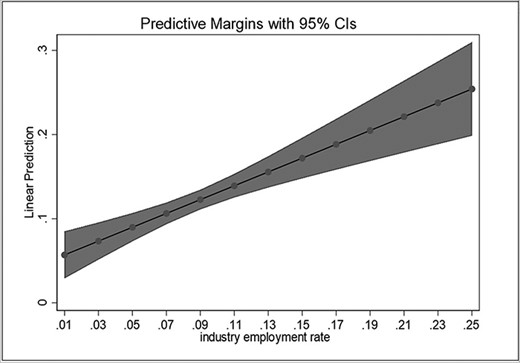
Predicted effect of industrial employment rates.
Quadratic estimates.
In our modeling strategy, we begin with simple models, increasingly adding complexity and sources of variation, as well as controlling for additional factors. The structure of the dataset motivates the selection of the alternative models chosen; as different models present different statistical trade-offs, Table 1 as well Appendices Tables A2–A4 report results for an array of specifications. As discussed in Inequalities and pandemic policy outcomes, we identified two main pathways through which economic disparities and inequality may affect the intensity of the pandemic: First, economic disparities are indirectly captured by the structural aspects of the labor market (in this case share of individuals employed in the industrial sector on the one hand, and the share of individuals employed in services on the other). Second, income inequality is directly captured by the distribution of income across the deciles of the population. Against this backdrop, Model A1 is a simple baseline OLS estimation with no constraints, to assess the baseline effects of our variables of interest. The first pathway is modeled by the share of the working-age population employed in the industrial sector, while the second pathway is modeled by the average per-capita income in the NUTS2 regions. In order to assess the robustness of the estimates across models as well as to isolate the effect of certain variables, we add several variations over the baseline. Model A2 replicates the same unconstrained model, using regional income inequality instead of average regional income, to better catch economic disparities. This alternative baseline specification offers higher precision in estimating inequality, at the cost, however, of cutting the number of observations by a half.2 Model A3 builds upon Model 2, introducing clustering of the standard errors at the country level, to control for the nested nature of the data. Clustering the standard errors at the country level allows us to account for differences in groups that may display common patterns (for instance, regions nested in countries) without introducing fixed effects, which may comport a loss of degrees of freedom and may lead to overfitting (model A7 reports the estimates for such model). For the same reason, model A4 is identical to Model A3, but with regional clustering instead of country-clustering of Standard Errors, to check whether results remain consistent when individual-level clustering is introduced. A fixed-effect estimator with regional fixed effects is reported in Appendix Table A2.3
Continuing to increase the precision of the model, Models A5 and A6 are versions of Model A3 controlling, respectively, for behavioral adaptation of the population through increases/decreases in mobility to work, measured through the Google Mobility Index, and for policy adaptation by governments, measured through changes in the Stringency Index, so to assess whether the estimates are robust with regard to important potential confounders. The Oxford stringency index is taken with a lag since stringency policies are reactionary rather than anticipatory to the evolution of the pandemic. Model A7 is equal to Model A3 but uses country fixed effects rather than clustering of the standard errors at the country level. Finally, Model A8 is a random-effects regional panel model with country fixed effects.
The results of these estimations are reported in Table 1 below. Overall, there are significant effects of economic disparities on mortality, such as the labor market preexisting structure, and, to a relatively lesser extent, by income inequality. Despite these effects being significant, the overall explained variance of excess mortality is naturally relatively limited, with the exception of the model controlling for behavioral adaptation (Model a5); economic disparities, as modeled here, explain only a fraction of the variance of excess mortality. This is understandable, particularly as the crisis in question is highly complex and builds on an array of intricate societal, economic, and epidemiological conditions.
Of the two pathways theorized in Inequalities and pandemic policy outcomes, the income distribution parameter—although obvious- seems relatively less prominent. The income effect is only statistically significant when included as inequality, despite the loss of some regions due to data availability. Including inequality improves the fit of the model, but the significance of the effect disappears when accounting for the nested structure of the data, either with clustering or with fixed effects. By contrast, the effect of industrial employment remains by far the strongest predictor and maintains a high statistical significance across all specifications (less than 1% chances of the effect being equal to 0 in Models 1–5). Figures 1 and 2, as well as models b1 and b2 in Appendix Table A2, illustrate such an effect: the regions with higher employment rate in industry4 tended to have higher excess mortality than the other regions.
As a counterfactual to this logic, model b3 in Appendix Table A2 shows the effect of services and retail employment. As expected, the share of the population employed in services and retail—which could work from home or was subsidized to close operations at the peaks of infection- is strongly and significantly negatively correlated with excess mortality, lending credibility to our intuition that, in fact, the employment characteristics of a jurisdiction do matter. This supports the fundamental intuition behind our labor market pathway: industrial activities cannot be easily performed remotely, and therefore industrial workers might have been disproportionately affected by the pandemic. This intuition remains supported also when controlling for changes in mobility and stringency, lending credibility to the idea that industrial workers were mostly only marginally affected by lockdowns; model b3 in Appendix Table A2 further controls for additional factors, such as median age and availability of hospital beds; while important, neither of these does alter the main result. While one should be wary of ecological fallacy—predicting individual-level effects from aggregate trends—our results point toward such effect, which should then be evaluated by future individual-level analysis once detailed data on the pandemic is made available to the public.
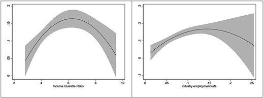
As shown, the precision of the estimate declines as industrial employment rates grow. While this is in part an effect of the lower number of regions with higher industrial employment rates, it may also be due to the presence of nonlinear effects. It may be, in fact, that regions with very high levels of income inequality or industrial employment share are somewhat less vulnerable. To test this, we explore a set of nonlinear models (Table A3 in Appendix). Models c1–c3 are simple variations over Model A3. Model c1 allows for nonlinear employment effects, Model c2 allows for nonlinear income effects, and Model c3 for both. Model c4 incorporates the behavioral and policy controls, capturing the intensity of the lockdown measures as well as the actual workers' mobility. Finally, Model c5 uses regional clusters instead of country clusters. Adopting a quadratic model substantially increases the fit of the estimation, for both the income and the employment parameters. These effects are best appreciated graphically: Figures 2A and B show the evolution of the effect of industrial employment share and income inequality if we allow such effects to follow nonlinear patterns.
For both pathways of inequality, the use of nonlinear specifications somewhat improves the fit, especially for income inequality estimations. These results, however, require some interpretation. When it comes to income inequality, three regions display a level of income inequality of 8 or above: the Yugozapaden region in Bulgaria, Sicily in Italy, and the development region of Nord-Est in Romania. For example, the Bulgarian region includes the richest areas of the country, including Sofia, which are likely to have access to far better public services than the rest of the country. Similarly, Sicily has the second healthcare spending as a percentage of their regional GDP in Italy. Furthermore, the insular nature of the region may have helped, especially in the first days of the pandemic, when mobility was heavily restricted throughout the country. With regard to industrial employment rate, the effect is mostly driven by small regions and exclaves, whose populations are relatively small and isolated. Among those, we find Ceuta, Melilla (Spain), Åland (Finland), and Mayotte (France). While not all regions with very high industrial employment are exclaves (for instance, Central Moravia and Western Moravia in the Czech Republic are also included), it is likely that the descendant trajectory of the nonlinear estimate is driven by the isolated nature of these exclaves.
As our results show, economic disparities had a clear impact on the outcomes of the COVID-19 crisis. While different parameters by which such disparities manifest show relatively varying levels of impact, their tangible effects warrant further consideration and discussion. In the next section, we elaborate on the caveats to be considered and the implications of such findings for policymaking.
Discussion and implications
Our results suggest that economic disparities within societies do have visible implications for how they fared during the COVID-19 crisis so far, particularly as the crisis mandated the engagement in behavioral and lifestyle adjustments. In this study, we found substantial evidence as to the impact of economic disparities on excess mortality. In this case, economic disparities (manifested in labor market structure) meant that regions with a higher share of industrial employment have disproportionately suffered from the pandemic. This effect is present yet relatively less visible if we use a pure income inequality lens (expressed through income quantile ratio, for example), but significant, nonetheless. Income inequality is always statistically significant when estimated in a nonlinear model, and—depending on the model—can be significant also in linear setups. We believe that the fundamental reason behind this could be that many regions of high inequality are relatively rich with respect to their countries, which likely provides them with better healthcare facilities. This in turn can relatively contain or dampen mortality rates. Hence, the curved nature of the relationship between income distribution and the pandemic comes as no surprise. These results remain robust even after controlling for a number of factors, including behavioral adaptation (as captured by Google community mobility data), policy stringency (as captured by the Oxford Stringency Index), and a number of alternative modeling choices (Appendix Tables A2–A4).
Overall, even though we find clear evidence suggesting that these influences of economic disparities are at work, the total explained variance can be perceived as relatively limited if viewed in absolute terms. In other words, while economic disparities are evidently associated with disproportionate death rates, there are also other important factors at work. In particular, accounting for behavioral effects- such as mobility to work- substantially improves the fit of the model. However, these findings should be understood within the larger context and inherent nature of the crisis at hand. The COVID-19 crisis is a complex, hard-hitting, large-scale, and socially embedded crisis (Zaki & Wayenberg, 2021), thus no single mechanism or factor can be solely attributed to explaining its key outcomes to an almost full extent. Hence, we argue that the exploration of a set of intricate and interwoven mechanisms and pathways (in this case, one of which is economic disparity) yields a better value for nuanced policymaking and lesson drawing. This takes us to the second part of our earlier inquiry, that is: How can these findings contribute to enhancing crisis policymaking within such contexts? We leverage our findings to provide a central recommendation to policymakers pertinent to acknowledging the multidimensionality of policy issues and within such contexts.
Multidimensionality of policy issues and policy designs
Our findings add to a growing stream of literature that emphasizes the multidimensional, complex, and creeping nature of some contemporary policy issues, such as the COVID-19 crisis (Boin et al., 2020). Within the context of this crisis (as well as others of similar features), our results highlight the need for dynamic contextual and societal configurations to be considered in issue definition, situational synthesis, and subsequently crisis policymaking. While policy instruments such as NPIs involve seemingly global technical standards (physical distancing parameters, standard personal protective equipment, work from home mandates, etc.), they interact with different societal, sectorial, and behavioral contexts (Zaki & Wayenberg, 2021). This process of interaction can create varying distributional effects for different groups and regions which consequently impact the ability of critical policies to achieve their desired objectives. Including behavioral, economic; and labor market experts in consultation committees can improve policymakers’ capacity to provide prompt effective responses to such crises and enhance perceived policy legitimacy and compliance. This becomes particularly important as perceptions of policy legitimacy are often constructed in relation to societal contexts at local levels (Connelly et al., 2006; Leino & Peltomaa, 2012). Overlooking these dynamics can be detrimental given the recognized impact of perceived legitimacy on compliance to policies (e.g., Siddiki, 2014).
Concluding remarks and limitations
While our results are robust across a range of modeling variations, they need to be interpreted with the context in mind. First of all, they cannot be interpreted in a causal fashion: our results show an association between variables, but do not necessarily identify a strong causal link between inequality and pandemic intensity. In terms of data availability, there are some issues to be considered. For example, classical GINI indices are only available at national level; their lack of variation within countries renders them unsuitable for non-longitudinal research. Similarly, additional data needs to be reported if future research is to account for more complex nuances of such crises at a large scale. This includes for example regionally disaggregated data on Long Term Care facilities (LTCs), among several other indicators. Regional economic data are also relatively scarce, and these data may not be missing at random. Similarly, while the Oxford university stringency index offers a robust, comparable, and widely acknowledged account of taken measures, data across standardized subnational regional units of analysis are yet to be reported.
Furthermore, one needs to acknowledge that while excess mortality is one of the most functional approaches to handle challenging attribution issues within the context of difficult cross-regional comparisons, it still potentially misses on some subtle changes in mortality for example due to mortality decreases during lockdown resulting from reduced traffic flows, etc. Its net and aggregate nature enables country comparisons, but at a cost of precision.
In terms of methodological caveats, it is important to treat our results as preliminary at this stage. First, even though economic disparity data is sourced before the pandemic (and therefore enables us to exclude reverse causality), we cannot fully exclude spurious correlations. Second and not only related to this particular study, readers should also be careful in directly transposing the results to the individual level: without individual-level data on excess death rates among professional and income groups, inferring individual behavior from the aggregate patterns revealed in our results would lead to a risk of ecological fallacy (hence micro-level transpositions are not within the scope of this study). Furthermore, this work does not investigate the individual characteristics which may lead to higher excess mortality: it would be wrong to infer from our results that societal factors are more important than individual elements such as behavioral choices, existing pathologies, old age, and others. As such, our study points out that some societal factors seem to be playing a role and should be considered as complements to individual characteristics when looking at the broad evolutions and outcomes of the pandemic.
These limitations notwithstanding, our findings provide a comprehensive and robust evidence of the impact of economic disparities on the state of the pandemic in Europe and can provide policymakers with key insights when viewed within the purview of what they intend to convey at the macro and meso levels.
Conflict of interest
None declared.
Appendix
Descriptive statistics of key variables.
| Variable | Nr. of regional observations | Mean | Std. Dev. | Min | Max |
|---|---|---|---|---|---|
| Population (1000s of people) | 15,567 | 3969.893 | 8100.169 | 29.884 | 83,166.71 |
| Excess mortality (p-scores) | 15,544 | 0.110735 | 0.279579 | −1 | 4.80304 |
| Income Quintile Ratio | 8081 | 4.876822 | 1.374734 | 2.8 | 9.5 |
| Income (1000s of Euros) | 14,943 | 15.33929 | 3.748837 | 5.8 | 23.6 |
| Material and Social Deprivation (% of population) | 10,172 | 14.26738 | 12.00166 | 1.5 | 56.2 |
| Industry employment rate (% of working-age population) | 15,359 | 0.076511 | 0.036081 | 0.012306 | 0.255059 |
| Share of population at risk of poverty (% of population) | 11,563 | 17.17839 | 7.063376 | 2.9 | 41.4 |
| Oxford Stringency Index (index) | 14,371 | 49.83409 | 25.50262 | 0 | 96.3 |
| Google Work Mobility index (index) | 13,848 | −26.045 | 15.6315 | −75.5714 | 7.571429 |
| Services employment share (% of working-age population) | 11,959 | 0.1051752 | 0.0291539 | 0.0261718 | 0.256356 |
| Median age | 10,399 | 12.14851 | 19.80169 | 0.117 | 188.909 |
| Hospital beds (1000s of beds) | 11,023 | 43.64848 | 3.771419 | 17.7 | 51.4 |
Robustness checks for baseline models.
| b1 | b2 | b3 | |
|---|---|---|---|
| Variables | Base model, regional fixed effects | additional control variables | Replacing industry for services |
| Industry employment rate | 22.43** | 0.544*** | – |
| – | (11.44) | (0.116) | – |
| Income quintile ratio | – | 0.00307 | 0.000604 |
| – | – | (0.00322) | (0.00353) |
| Population | – | −0.0253*** | −0.0329*** |
| – | – | (0.00372) | (0.00360) |
| Hospital beds | – | 0.008*** | 0.000*** |
| – | – | (0.001) | (0.000) |
| Median age | – | 0.00267* | 0.00266* |
| – | – | (0.00142) | (0.00145) |
| Mobility to work (%. change) | – | −0.00482*** | −0.00479*** |
| – | – | (0.000260) | (0.000274) |
| Services employment rate | – | – | −0.523*** |
| – | – | – | (0.178) |
| Region fixed effects | omitted (298 region coefficients) | – | – |
| Constant | −1.475* | −0.198*** | −0.0963 |
| – | (0.798) | (0.0609) | (0.0643) |
| Observations | 13,703 | 4530 | 3992 |
| R-squared | 0.068 | 0.090 | 0.092 |
p=.01.
p=.05.
p=.1.
Quadratic estimates.
| c1 | c2 | c3 | c4 | c5 | |
|---|---|---|---|---|---|
| Industrial employment | Income | Income and industrial employment (clustered standard errors: national level) | Income and industrial employment (clustered standard errors: national level) +mobility and stringency controls | Income and industrial employment (clustered standard errors: regional level) | |
| % of population employed in industry | 1.829*** | 0.682** | 1.966*** | 2.893*** | 1.965*** |
| (0.603) | (0.281) | (0.603) | (0.799) | (0.330) | |
| Industrial employment (squared) | −6.149** | −6.657*** | −9.425*** | −6.653*** | |
| – | (2.309) | – | (2.239) | (2.997) | (1.285) |
| Income quintile ratio | 0.00676 | 0.0649* | 0.0728** | 0.109** | 0.0728*** |
| – | (0.00596) | (0.0336) | (0.0326) | (0.0393) | (0.0223) |
| Income Quintile ratio (squared) | – | −0.00508* | −0.00573** | −0.00860** | −0.00573*** |
| – | – | (0.00269) | (0.00252) | (0.00323) | (0.00184) |
| Population (millions) | 0.000275 | 0.000294 | 0.000104 | −0.000012 | 0.000103 |
| – | (0.000503) | (0.000507) | (0.000500) | (0.000576) | (0.000525) |
| Mobility to work (% change) | – | – | – | −0.00440*** | – |
| – | – | – | – | (0.00117) | – |
| Stringency index (6 weeks lag) | – | – | – | 0.000230 | – |
| – | – | – | – | (0.000307) | – |
| Constant | −0.0206 | −0.130 | −0.202* | −0.466*** | −0.202*** |
| – | (0.0479) | (0.114) | (0.116) | (0.114) | (0.0696) |
| – | – | – | – | – | – |
| Observations | 8523 | 8523 | 8523 | 5940 | 8524 |
| R-squared | 0.012 | 0.011 | 0.015 | 0.083 | 0.015 |
Standard errors in parentheses.
p<.01.
p<.05.
p<.1.
Additional estimates & alternative inequality measures.
| d1 baseline (model 3) | d2 multilevel model (2 levels) | d3 dynamic model | d4 industrial employment only | d5 income quintile ratio only | d6 material & social deprivation only | d7 poverty risk only | |
|---|---|---|---|---|---|---|---|
| Excess mortality (previous week) | 0.864*** | ||||||
| (0.0104) | |||||||
| % of population employed in industry | 0.647** | 0.372** | 0.152*** | 0.470** | |||
| −0.266 | (0.153) | (0.0299) | −0.187 | ||||
| Population (millions) | 0.000434 | 0.000529 | 0,000 | 0.00057 | 0.000491 | 0.000561 | 0.000633 |
| −0.000514 | (0.000401) | (0,000) | −0.000594 | −0.000505 | −0.000558 | −0.000571 | |
| Income quintile ratio | 0.00636 | −0.00452 | 0.00155*** | 0.00338 | |||
| −0.00602 | (0.00454) | (0.000502) | −0.00735 | ||||
| Material & social deprivation | 0.000143 | ||||||
| −0.000829 | |||||||
| At Risk of Poverty | −0.000333 | ||||||
| −0.00137 | |||||||
| Constant | 0.0274 | 0.0846*** | 0.00188 | 0.0724*** | 0.0945* | 0.110*** | 0.119*** |
| −0.0483 | (0.0312) | (0.00434) | −0.0157 | −0.0503 | −0.0233 | −0.0304 | |
| Observations | 8523 | 8523 | 8360 | 15,855 | 8523 | 10,551 | 11,903 |
| No. of groups | 29 | ||||||
| R-squared | 0.009 | 0.742 | 0.005 | 0.001 | 0 | 0.001 |
p=.01.
p=.05.
p=.1.
A: Change in death rates in low- industrial employment regions. B: Change in death rates in high- industrial employment regions (exclaves excluded).
Main Data Sources
Excess Mortality: Manually Calculated from https://ec.europa.eu/eurostat/statistics-explained/index.php?title=Mortality_and_life_expectancy_statistics
Population employed in industry:https://ec.europa.eu/eurostat/statistics-explained/index.php?title=Employment_-_annual_statistics
Population (millions):https://ec.europa.eu/eurostat/statistics-explained/index.php?title=Population_and_population_change_statistics#EU-27_population_continues_to_grow
Income quintile ratio:https://appsso.eurostat.ec.europa.eu/nui/show.do?dataset=ilc_di11&lang=en
Material & social deprivation:https://ec.europa.eu/eurostat/web/products-eurostat-news/-/DDN-20171212-1
Gini Coefficients:http://appsso.eurostat.ec.europa.eu/nui/show.do?lang=en&dataset=ilc_di12
People At Risk of Poverty:https://ec.europa.eu/eurostat/databrowser/view/t2020_50/default/table?lang=en
Policy Stringency:https://www.bsg.ox.ac.uk/research/research-projects/covid-19-government-response-tracker
Healthcare Capacity Data:https://ec.europa.eu/eurostat/statistics-explained/index.php?title=Healthcare_resource_statistics_-_beds
Median population age:https://ec.europa.eu/eurostat/statistics-explained/index.php?title=Population_structure_and_ageing
Endnotes
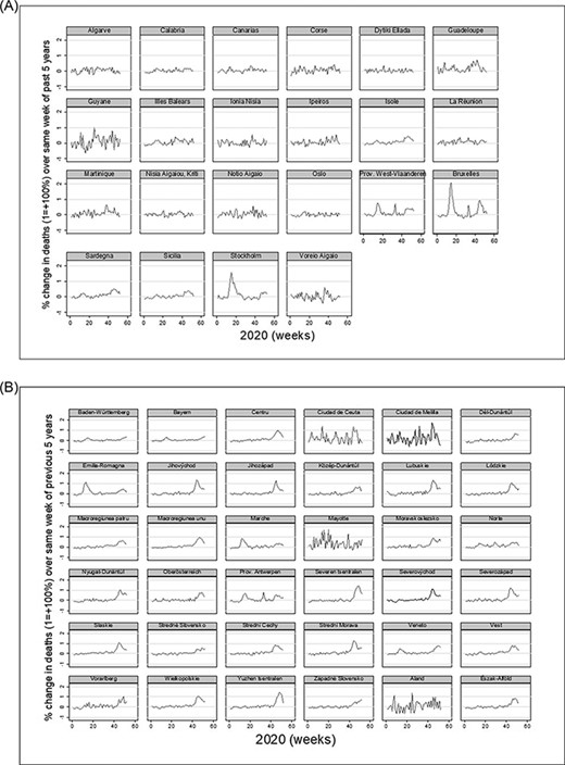
NUTS 2 Nomenclature of Territorial Units for Statistics) regions are the European Union’s defined basic regions for the application of regional policies. Figure A1 in appendix depicts the weekly excess mortality in high- and low- industrial employment regions.
Such differences in reporting not only reduce the quality of the estimation by reducing the sample size, but also risk of introducing biases as missing information might be non-random.
Note that introducing regional fixed effects- over 300 variables- severely decreases the Degrees of Freedom.
These include NACE review 2 codes B-E, excluding construction and services.
