Modelling Cross-Shore Shoreline Change on Multiple Timescales and Their Interactions

Abstract

In this paper, a new approach to model wave-driven, cross-shore shoreline change incorporating multiple timescales is introduced. As a base, we use the equilibrium shoreline prediction model ShoreFor that accounts for a single timescale only. High-resolution shoreline data collected at three distinctly different study sites is used to train the new data-driven model. In addition to the direct forcing approach used in most models, here two additional terms are introduced: a time-upscaling and a time-downscaling term. The upscaling term accounts for the persistent effect of short-term events, such as storms, on the shoreline position. The downscaling term accounts for the effect of long-term shoreline modulations, caused by, for example, climate variability, on shorter event impacts. The multi-timescale model shows improvement compared to the original ShoreFor model (a normalized mean square error improvement during validation of 18 to 59%) at the three contrasted sandy beaches. Moreover, it gains insight in the various timescales (storms to inter-annual) and reveals their interactions that cause shoreline change. We find that extreme forcing events have a persistent shoreline impact and cause 57–73% of the shoreline variability at the three sites. Moreover, long-term shoreline trends affect short-term forcing event impacts and determine 20–27% of the shoreline variability.

1. Introduction

Sandy beaches are constantly adapting to changing wave forcing over a variety of temporal scales [1,2,3], which can be traced in changes in cross-shore shoreline positions. Coastal variability, and particularly erosion, can expose human and ecosystems in the littoral zone to risk, which implies that understanding and predicting shoreline evolution is of paramount importance. However, it is not straightforward to predict shoreline variability at a multitude of natural temporal scales from storm events to seasonal and inter-annual evolution because the governing processes are complex. On top of that, there is often a lack of sufficient observations of shoreline change, which hampers the prediction of shoreline variability even more. Furthermore, these observational strategies generally focus on a particular spatial-temporal scale (e.g., monthly observations at a certain shoreline transect or short-term field campaigns [4,5]). The same is true for many of the equilibrium-based shoreline models [6] that are optimized during the calibration process for the single most dominant timescale of shoreline variability in the training set. Quite often this results in models being skillful at either the short-term (e.g., storm or monsoon) timescale or optimized for the longer (seasonal to inter-annual) timescales [7]. Addressing all the timescales together is a major challenge and as a result, current understanding on how the shorelines respond to different timescales and how these timescales influence shoreline change is limited.

The understanding and prediction of coastal evolution are often simulated using models that simulate hydrodynamics linked to morphodynamics that can roughly be divided into three categories: the more complex and time-consuming process-based models [8,9,10,11], hybrid models (usually based on the equilibrium concept [6,12,13]) and, more recently, machine learning models [6,14]. Each of these models are typically bound to the dominant spatial and temporal scales of key processes to model, and as a result they struggle, or become too computational expensive, in order to account for dynamics at different timescales. Hybrid (equilibrium) models are generally more computationally efficient in comparison to process-based models and have been proven reliable on seasonal or inter-annual timescales to simulate shoreline behavior [15,16,17,18,19]. However, they typically account for a single dominant physical process and need a large, site-specific dataset for calibration purposes [20]. Another limitation to these models is that only coastal processes observed during the calibration timeframe are accounted for [21]. Moreover, hybrid models do not explicitly account for all individual processes that drive shoreline change but seek an overall behavior pattern as a response to the different processes.

The single-timescale equilibrium ShoreFor model [17] (SF-ST, see Appendix A for a model description) seeks the best relation between the raw wave forcing and raw shoreline position data through the fitting of several calibration parameters (c and φ) using the knowledge of how the beach responds to incoming wave forcing. For example, a beach in equilibrium with the current and antecedent forcing conditions will try to adapt to a new equilibrium if wave conditions change, like in the case of a high-intensity forcing event (e.g., a storm or monsoon) impacting the coastline. During such an event, the beach will erode and the shoreline moves landward. The new established shoreline is then more in equilibrium with the prevailing forcing. However, several characteristics of the high-intensity forcing event play a role in how the (modelled) shoreline position responds to the considered wave forcing. The first aspect is the forcing duration: only if the duration is long enough (i.e., stationary conditions), a new equilibrium is established. Secondly, the intensity of the wave forcing determines how far the beach retreats. Thirdly, in the case of multiple high-intensity forcing events, the sequence of these forcing events (e.g., a storm cluster) determines to a large extent the shoreline change [16]. A prerequisite, for the sequencing to be important, is that the beach has no time to fully recover in between the high-intensity forcing events that make up the cluster [22,23]. To what extent a beach recovers from the antecedent high-intensity forcing conditions mainly depends on the characteristics of the post-storm hydrodynamic conditions relative to the antecedent conditions [24].

Within SF-ST, the key model-free parameter is the memory decay factor (φ), which indicates the single most dominant response time of cross-shore sediment exchange. However, due to this single memory decay factor, model skill deteriorates considerably if multiple dominant forcing and beach response timescales are present [3,19,21]. Moreover, the SF-ST model is only applicable on locations where wave-driven, cross-shore processes dominate sediment transport and where anthropological influences are minimal [17]. SF-ST was originally established using data in microtidal environments (see [17]), but the subsequent model of [18] was established covering a wide range of tidal ranges. Furthermore, [25] showed that the model yields significant skill in reproducing post-storm recovery in a macrotidal environment as well. Nevertheless, in this paper, model training sites with a limited tidal range are used in order to minimize the influence of the tide on the shoreline location (see Section 2).

Recent studies identified the persistent nature of short wave events on longer beach response timescales [3,22,23,26,27,28]. This link between the different timescales is often missing when modelling the seasonal to inter-annual evolution of the coastline and storm impact persistence. For example, extremes (e.g., storms and tropical cyclones) have both a transient and persistent impact, individually or in sequence [27]. Moreover, [22] showed the influence of average winter storms on beach response and revealed that not only the storm energy is important, but also the frequency of recurrence, highlighting interactions between short-term storms and long-term evolution. They showed the importance of the recurrence frequency of extremes to beach erosion and post-event reconstruction, such that the shoreline retreat was most governed by the first storm in the sequence, while the impact of subsequent forcing events was less pronounced (low cumulative impact), something that is also observed in [29] and follows the general equilibrium response of a beach [16,17,18]. Furthermore, a main outcome of recent studies in tropical South East Asia [3,30] is the long lag (50–60 days) observed between monthly-averaged waves and shoreline location, while the envelope of intra-seasonal monsoon events is in closer phase with the shoreline location. Hence, the shoreline variation appears to be in equilibrium with energetic wave conditions, rather than the monthly-averaged waves. In this paper, we aim to account for these processes by linking different timescales in forcing and response.

Recent work by [7,19] showed that timescales of beach change and forcing may be temporally dependent, with beaches undergoing rapid adjustment to the changes in the dominant wave forcing over time and where single-timescale models can fail to capture the observed shoreline signal. The authors of [19] showed that the beach at Gold Coast (Australia) was subjective to two different beach response frequencies corresponding to two consecutive 4-year time periods. The movement of the shoreline at this site changed from a seasonally-dominated mode (annual cycle) to a storm-dominated (∼monthly) mode. The authors of [7] used an approach whereby model-free parameters are allowed to vary in time, adjusting to potential non-stationarity in the underlying model forcing. They revealed that time-varying model-free parameters are linked through physical processes to changing characteristics of the wave forcing. Here, we aim to implement the fact that beach response to dominant timescales in wave forcing may be dependent on large timescale shoreline variations by using a time dependent model-free parameter.

In this paper, we evaluate to what extent multiple timescales of dominant forcing and beach response behavior co-exist and to what extent such behaviors can interact with different timescales of forcing and response. We aim to improve cross-shore multi-timescale shoreline predictions by using the single-timescale ShoreFor model [17] (SF-ST, see Appendix A for a model description) as a baseline model.

2. Model Training Sites Covering Different Wave Environments

To train the SF-ST model, shoreline location and wave measurements are required. A source of shoreline data are shore-based video cameras that generally collect data during daylight on a 30 min basis [31]. In comparison to shoreline-walking GPS surveys, these video-based shorelines provide significantly better temporal resolution, which makes video-derived shorelines particularly suitable to study the importance of different, multiple, response timescales [2,32].

In order to make the video data suitable for SF-ST and to cover a wide range of timescales (1 day to inter-annual timescales), the shoreline dataset at Nha Trang and all wave forcing datasets are interpolated (upsampled, corresponding to the value every 24-h), such that they have a temporal resolution of 1 day. The shoreline datasets at Narrabeen and Tairua have a daily interval corresponding to the procedures outlined in [6,33], respectively. Moreover, the raw shoreline position data is detrended by a second-order polynomial in order to filter out shoreline trends which have a larger temporal scale than the duration of the dataset. The importance of multiple beach response timescales will be investigated at three different study sites: Narrabeen (Australia), Nha Trang (Vietnam) and Tairua (New Zealand). These sites were chosen to cover different wave environments and for the availability of daily shoreline data. All three beaches are subjected to a small tidal range (microtidal, <2.0 m, <1.6 m and <2.0 m, respectively), such that SF-ST has an optimal model performance [3,34,35], respectively. Moreover, the beach dynamics are either dominated or largely influenced by cross-shore processes. Furthermore, major differences between the wave conditions are present at the three study sites. The wave climate at Narrabeen consists of small (daily) timescale storms (and swell waves) and a larger temporal scale, but less intense seasonal cycle. At Nha Trang, three distinct wave forcing timescales are present: typhoons (daily), monsoons (monthly) and a seasonal variation (annual). At Tairua, the wave climate is largely influenced by small timescale storm and swell waves [36].

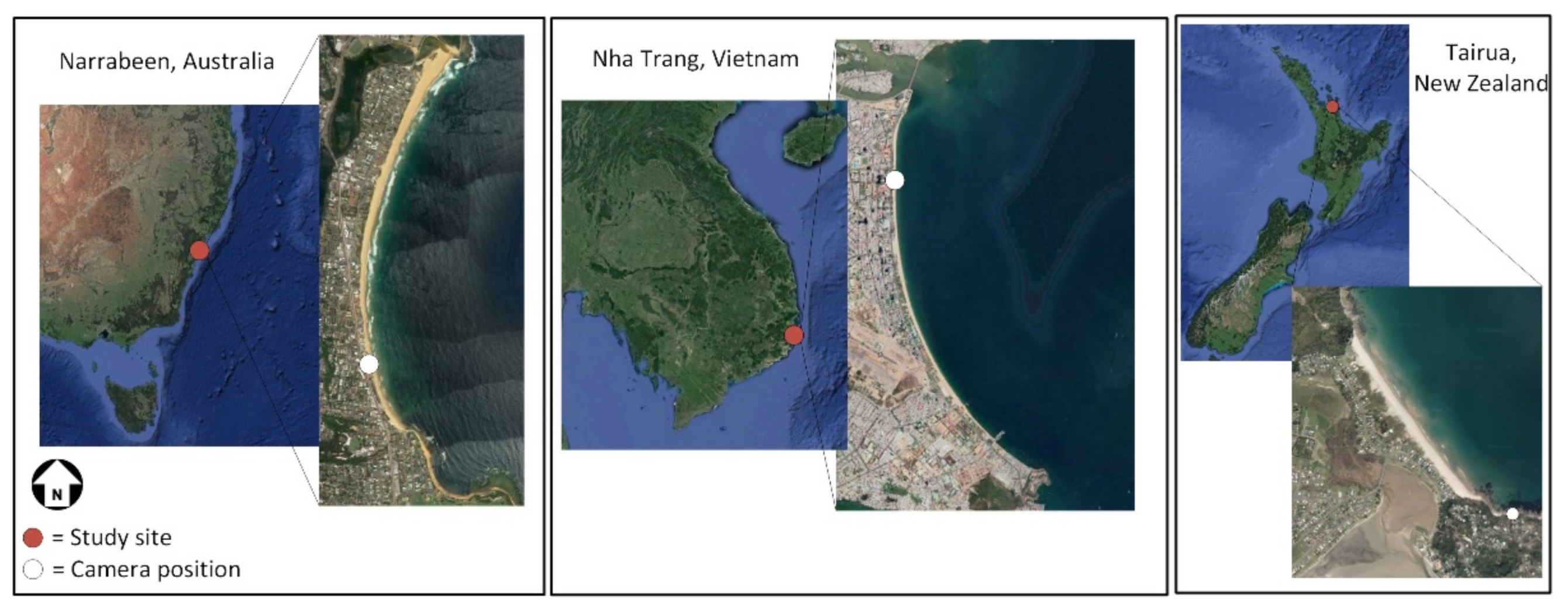
2.1. Narrabeen-Collaroy Beach, Australia

The Narrabeen-Collaroy beach (34° S) is situated near Sydney in the southeast of Australia (Figure 1). The embayed beach is bound at the north and south by two headlands. Narrabeen beach is situated in the north of the embayment and Collaroy beach is situated in the south. In 2004, an ARGUS system [31,37] was installed, from which shorelines can be extracted. In this paper, alongshore averaged shoreline data a bit southwards of the center of the embayment is used (2400 m to 2800 m from the northern edge of the embayment), in line with previous studies at this beach [17,33]. Narrabeen beach is characterized by sand with a D50 of 0.4 mm. The wave climate is largely influenced by swells from the SSE (mean H_s = 1.6 m and mean T_p = 10 s). Additionally, the wave climate consists of larger waves (H_s = 3 m) that originate from storm events and can hit the coastline in any direction. For example, in June 2007 an energetic storm sequence hit the coastline and caused roughly 35 m of shoreline retreat [38]. Furthermore, a small seasonal cycle is present with on average higher waves in the Australian winter and milder waves in the Australian summer months [38]. On larger timescales, effects of El-Nino Southern Oscillation (ENSO) can play a role as well [37,39,40]. In this study, nearshore wave timeseries at the 10 m depth contour are used.

2.2. Nha-Trang Beach, Vietnam

A video system [41,42] was installed in 2013 at Nha Trang beach in Vietnam (12° N) (Figure 1). The camera location is considered far enough for the beach not to be influenced by the edges of the bay [3]. Cross-shore shoreline positions are estimated from this camera data on a daily basis. The shoreline location used in this paper is retrieved by alongshore averaging the video-derived shoreline data (over 75 m) from the northern part of the bay relative to the camera location. Nha Trang beach is characterized by sand with a D50 of 0.3 mm. Interestingly, the tropical wave climate at Nha Trang is characterized by multiple wave conditions with a distinct timescale, of which the seasonal variation is the most pronounced. The offshore annual mean significant wave height (H_s) is 0.95 m, with an associated averaged peak period (T_p) of 6.2 s. Typhoons typically occur on average 4–6 times per year between August and November. Intriguingly, typhoons were abundant in 2013, where the most extreme one occurred in November of that year [3]. The wave climate is also characterized by summer and winter monsoons, where the summer monsoons mainly consist of wind waves and the winter monsoons of swell waves. The winter monsoons (October to April), which do not occur at the same time as the typhoons, can generate waves up to 4.0 m, which can heavily affect shoreline change. During fall and winter (October to April), the mean H_s is 1.2 m and T_p is 6.8 s, while during spring and summer (May to September), the mean H_s is reduced to 0.6 m, with a shorter T_p below 5 s [30].

2.3. Tairua Beach, New-Zealand

Tairua Beach is situated at the east coast of New Zealand’s northern island (37° S) (Figure 1). This 1.2 km long beach is situated in between two headlands, where on the southern headland, a video camera was installed in 1998. In this study, high-resolution shoreline data (alongshore averaged over the bay: 1050 m, see [6]) is used, which is extracted from those camera images. Tairua beach is characterized by sand with a D50 of 0.3 mm. The beach is subjected to easterly and northeasterly swell and storm waves [35]. The offshore wave climate has a mean H_s of 1.4 m, and can reach values of up to 6 m during storm events [43]. In the winter (southern hemisphere) of 2000 a series of huge storms occurred, which caused erosion of the shoreline of roughly 20 m [44].

3. Implementing Multiple Timescales and Links between Timescales in the Cross-Shore Shoreline Model

We propose four steps to implement multiple dominant forcing and beach response timescales within the SF-ST model and to assess its performance. The first step is to distinguish timescales in the measured data using a filter function and subsequently determine which timescales are dominant in the raw forcing and shoreline position signals (Section 3.1). Then, an approach to implement these multiple dominant timescales in the SF-ST model is proposed (Section 3.2). This implementation uses a threefold correspondence between the isolated timescales of the wave data to the isolated timescales in shoreline data where the timescales that are smaller, identical or larger are linked in a direct forcing, upscaling and downscaling procedure (Section 3.2.1, Section 3.2.2, Section 3.2.3, respectively). The combined model is referred to as ShoreFor Multiple Timescales (SF-MT). Subsequently, the modelling calibration and validation phases are elaborated in Section 3.3. In Appendix B, model skill assessment and performance are discussed.

3.1. Distinguishing Multiple Timescales

To distinguish timescales, the raw shoreline position and wave forcing (H_s, T_p) data is filtered using a running average filter with varying (enlarging) window sizes. The running average filter is used to allow for data gaps in the datasets. Per window, and hence timescale (i.e., 1 until the length of the timeseries, with steps of 1 day), a residual variance of the shoreline position and wave forcing timeseries is calculated. With residual variance of the filtered signals a temporal spectrum is constructed. In other words, we can plot the temporal spectrum as the (remaining) variance of all filtered signals as a function of the timescale. Dominant timescales are defined by the largest variance. In contrast to, for example, Fourier spectra, the linear superposition of all filtered signals is not equal to the raw signal since the filter function is shape preserving but not energy conserving. By dividing the filtered signals by a weighting value proportional to the window size of the running average filter, energy is conserved and the raw signal can be reconstructed through linear superposition. As a consequence, the energy (i.e., variability) for each filtered signal reduces, where the difference is largest for the largest timescales, because the window width increases with increasing timescales. A second temporal spectrum can be constructed from the resulting signals, which is used to construct timescale clusters by dividing the spectrum into bins (i.e., bands). These steps to distinguish timescales are summarized in Figure 2A–C.

When filtered wave forcing and shoreline position signals are directly related (i.e., on a corresponding timescale) using SF-ST, the corresponding calibration parameters and resulting modelled shoreline position signals are partly dependent on the variability of the related (input) signals. For example, the response value (i.e., c, Equation (A1)), becomes smaller if the variability of the wave forcing becomes larger (for the same shoreline signal), because the rate parameter (c) and wave energy flux (P) determine the magnitude of the shoreline response [18]. Hence, the variability of all (filtered) input signals has to be identical, when considering an inter-comparison of modelled shoreline position signals on multiple timescales. Therefore, timescale clusters are used, of which each cluster has an identical variability. To that end, the previously obtained spectrum is employed (Figure 2C) and will determine the number of timescale clusters that is used for the multi-timescale implementation. Timescale clusters are formed by dividing the obtained temporal spectrum into bins. Within such a bin a particular number of filtered signals can be found. The linear superposition of all filtered signals within a bin results in a timeseries which represents a particular timescale (i.e., a timescale cluster). The bin distribution is based on an equal amount of shoreline response variation within each bin. In this way, all resulting timescale clusters, which represent certain timescales, will have the same variance. The variability within a bin is equal to the signal with the largest variability in the spectrum, otherwise the variability of that signal does not fit within the bin. This means that only one filtered signal fits within the bin at the point corresponding to the peak of the spectrum. For other bins, multiple filtered signals can fit in a bin, because the variability of those individual signals is lower. The lower the local variability of the spectrum, the wider the bins, the more filtered signals fit within a bin (Figure 2D). Hence, the bin distribution is determined by adding up filtered signals (starting with the signal that has a timescale of 1 day), until that summation reaches the maximum variability of the bins. For the remaining filtered signals, a new bin is used. This procedure is continued up to the point where all filtered signals fall within a bin.

In the wave forcing spectra (i.e., the individual spectra for H_s and T_p), an identical bin distribution is used such that corresponding timescale clusters are formed. Thereafter, the different timescale clusters in the wave forcing data (H_s,i and T_p,i, where i indicates the timescale cluster) are related to ones in the shoreline data on multiple scales. The interactions between the wave forcing and shoreline position timescale clusters on multiple timescales are based on three approaches: the direct forcing, the upscaling and downscaling approach. The combined model is referred to as Shoreline Forecast Multiple Timescales (SF-MT).

3.2. Implementing Multiple Timescales

In this section, the multi-timescale implementation within the SF-ST model is governed by introducing the three separate terms: the direct forcing, upscaling and downscaling approach (Section 3.2.1, Section 3.2.2, Section 3.2.3, respectively). The direct forcing approach relates corresponding timescale clusters in the wave and shoreline position data. The upscaling approach accounts for the persistent effect of short wave events on the shoreline position. The downscaling approach accounts for the effect of the longer timescales in beach variation on the impact to shorter forcing events by introducing a time-dependent response factor.

3.2.1. Direct Forcing

In the direct forcing approach, all timescale clusters in the wave forcing data (H_s,i and T_p,i, where i indicates the timescale cluster) are related to corresponding timescale clusters in the shoreline position data (x_i), following:

$$\frac{d{x}_i\left(t\right)}{dt}=c_i\left(F^{+}\left({\mathrm{\varphi }}_i,t\right)+r_i{F}^{-}\left({\mathrm{\varphi }}_i,t\right)\right)$$

(1)

in which i indicates that corresponding timescale clusters in the wave forcing and shoreline position data are linked to each other, and calibrated by using a separate c and φ for every timescale cluster. Note that the standard single-timescale ShoreFor model (SF-ST, see Appendix A) is not adapted in the direct forcing approach (except for the linear trend term), but it is applied multiple times: for each timescale cluster with a distinct timescale. The linear trend term (b) is omitted from the model, because otherwise a linear trend will be present for every band. Within each band, no linear trend is present as the filter function only captures timescales which are smaller than the full length of the dataset. Hence, b should be zero when the full timeframe is considered. However, during the calibration phase only part of the entire dataset is used such that a (small) trend can be present. Subsequently, this trend will be assigned to b (or partly, depending on the wave characteristics). As this linear trend will be extrapolated during the validation phase, it will result in a wrong shoreline prediction as no trend is present over the full period.

3.2.2. Upscaling: The Long-Term Persistence of Short Timescales

To include the relation between small wave forcing timescales and larger timescales in shoreline response, as small timescale wave forcing events (e.g., storms or monsoons) can have a considerable and persistent effect on larger beach response timescales [3,26,27], an upscaling approach is proposed. This is described mathematically as follows:

$$\frac{d{x}_j\left(t\right)}{dt}=c_j\left(F^{+}{\left({\mathrm{\varphi }}_j,t\right)}_{i\to j}+r_j{F}^{-}{\left({\mathrm{\varphi }}_j,t\right)}_{i\to j}\right)$$

(2)

wherein the subscript indices i and j indicate the timescales: i is the small wave forcing timescale and j the larger timescale (j > i). The upscaling effect is indicated with an arrow. Hence, applied to the synthetic spectra in Figure 2E, i is equal to timescale cluster 1 (or 2) and where j can be equal to either II or III (or III). Note that all combinations (i.e., timescale interactions) are calculated. In this model improvement step the ShoreFor model equation has kept its original form (Equation (A1)), while only the forcing is represented differently.

This upscaling effect is evaluated by using an envelope (based on spline interpolation) of wave forcing timescale clusters that links the two different timescales. Figure 3 shows an example of an envelope (black-dashed) of a significant wave height timescale cluster (black-solid), where it is clearly visible that the envelope has a larger timescale than the wave height signal. A similar approach is followed for the wave period. The envelopes representing the wave height and wave period will be related to the corresponding shoreline timescale cluster (red-solid). The resulting modelled shoreline is represented by the red-dashed timeseries in Figure 3.

3.2.3. Downscaling: The Changing Response Efficiency of Short Timescales Due to Long-Term Shoreline Variations

The incorporation of the effect of large timescale shoreline variations on the efficiency with which smaller timescale wave forcing events induce cross-shore sediment transport is achieved by a so-called downscaling approach. This step ensures that smaller beach response timescales can be accounted for, if larger ones dominate. The downscaling approach is slightly adapted compared to SF-ST and can be mathematically described as follows:

$$x_i\left(t\right)=c_j\left(t\right){{\displaystyle \int }}_0^t\left(F^{+}\left({\mathrm{\varphi }}_i,t\right)+r_i{F}^{-}\left({\mathrm{\varphi }}_i,t\right)\right)dt$$

(3)

in which the subscript indices i and j indicate the timescales, where j > i. Note that c is now a function of time and has the shape of the time-varying shoreline signal with timescale j. Hence, applied to the synthetic spectra in Figure 2E, i is equal to timescale cluster 1 (or 2) in the wave data, and I (or II) in the shoreline data. Thus, the approach is similar to the direct forcing approach, but now c is time-varying and has the shape of the large timescale shoreline cluster II or III (or III). Note that all combinations (i.e., timescale interactions) are calculated.

The justification of the downscaling approach consists of three components: (1) the influence of large timescale shoreline variations on beach response to small timescale high-intensity forcing events as observed in measurements, (2) modelling of small beach response timescales with the direct forcing approach and (3) modelling of small beach response timescales with the downscaling approach.

When a high-intensity forcing event of a small temporal scale (e.g., storm/monsoon) impacts the coastline, the beach response can depend on whether that coastline is eroded or accreted on a larger temporal scale (e.g., due to a seasonal variation). Or stated otherwise, on the initial state of the beach [45]. For a beach in the state of erosion, a minor retreat of the shoreline location is expected due to the presence of a dissipative beach profile. For an accreted beach a larger beach response is expected [16]. If the period between two similar high-intensity forcing events is very small compared to the calibrated memory decay factor (<2φ), the direct forcing approach is already able to model the fact that the subsequent forcing events correspond to a different beach response. The (modelled) response to the second forcing event is lower, because the coastline is already closer to the equilibrium with the high-intensity forcing conditions. This is due to the dynamic equilibrium condition (Equation (A4)) which introduces a negative feedback mechanism (i.e., damping): the disequilibrium between the present and the antecedent forcing is lower during the second forcing event. This mechanism ensures that if two high-intensity forcing events approach the coastline shortly after each other, the cumulative shoreline recession is limited [17]. However, if the period between two similar high-intensity forcing events is considerably larger than the memory decay factor (>2φ), the direct forcing approach is not able to model a different beach response due to a different initial state of the beach (i.e., a varying shoreline location on a larger timescale). Due to the constant response factor (i.e., c_i; Equation (1)) and the large period between the two short high-intensity forcing events, the direct forcing approach will model two beach responses with the same erosional amplitude. Hence, no connection is present between the larger timescale shoreline variation and the modelled small timescale beach response to high-intensity forcing conditions.

To implement the dependency of small timescale beach response (to short high-intensity forcing events) on large timescale beach variations, a time-varying response factor is used (i.e., c_j(t); Equation (3)). This dynamic response factor represents the changing efficiency over time with which waves induce cross-shore sediment transport and is a function of the spatial separation between the shoreline and the more offshore sediment source (e.g., sand bar(s)). This spatial separation normally scales with the surfzone width imposed by the antecedent waves, with lower response rates for dissipating profiles (wide surfzone) due to the inefficient transfer of sediment between the more offshore region and the beach face. Conversely, as the more offshore sand supply is migrated closer to the shoreline (narrow surfzone; accreted beach), the sediment transport efficiency increases, facilitating faster response. Therefore, the dynamic response factor can be seen as an adjustment time scale and is a function of, for example, the current shoreline position, antecedent forcing conditions and morphological components such as sandbars. Therefore, within SF-MT the dynamic response factor has the shape of a large timescale shoreline signal, such that the response to a short high-intensity forcing event is higher (large sediment transport efficiency) when the beach (on a larger time scale) is accreted and lower (small efficiency) when the beach is already eroded.

Downscaling can be further illustrated by the timeseries in Figure 4. The dynamic response factor (c_j(t)) (black-dashed) has the shape of the considered large timescale shoreline variation to account for a variable sediment transport efficiency, because beach response to small timescale high-intensity wave forcing events (red-solid) can depend on this larger timescale shoreline variation (i.e., the initial state of the beach). The figure shows that if the shoreline on a larger timescale is accreted (e.g., October 2013, high dynamic response factor), the relative (compared to the wave forcing, black-solid) shoreline response on a smaller timescale (red-solid) is large (higher sediment transport efficiency). Conversely, if it is eroded (e.g., January 2014, low dynamic response factor), the relative shoreline response is low (limited sediment transport efficiency). The resulting modelled shoreline timeseries is indicated by the dashed red line in Figure 4B.

3.3. Model Calibration and Validation

The modelling of cross-shore shoreline change on multiple timescales is divided in two phases: model calibration and model validation. During model calibration the site-specific model-free parameters (c_i and φ_i) are determined using the wave forcing (H_s,i and T_p,i) and shoreline data (x_i), where the subscript i indicates the multiple predictions from the direct forcing, upscaling and downscaling approaches. At the time of model validation, wave forcing data is used as model input only and together with the calibrated parameters shoreline predictions are generated.

Table 1. Calibration and validation timeframes of the Narrabeen, Nha Trang and Tairua dataset, as well as the percentages of data gaps in the shoreline position data (based on daily data).

Dataset	Calibration Timeframe	Validation Timeframe	Data Gaps in Shoreline Position [%]
Narrabeen	1 August 2004/10 July 2010	11 July 2010/19 April 2015	25
Nha Trang	27 July 2013/31 December 2014	1 January 2015/1 November 2015	20
Tairua	2 January 1999 /31 December 2008	1 January 2009/31 December 2013	0

presents the calibration and validation timeframes for all three datasets. Furthermore, note the difference in the percentages of data gaps in the shoreline position data (the wave forcing data is continuous for all three study sites).

3.3.1. Calibration of the Downscaling Approach

While the calibration method for the direct forcing and upscaling approach for every timescale cluster is similar to that of the SF-ST model, the calibration method for the downscaling approach is slightly different considering that the dynamic response factor (c_j(t), Equation (3)) has the shape of a larger timescale shoreline signal. However, this dependency poses a problem as during validation the model must generate shoreline predictions which are solely based on wave forcing (shoreline data is not available as model input). Hence, a different approach is needed to generate the dynamic response factor (i.e., the larger timescale shoreline signal). Note that the modelled shoreline signals from the direct forcing and upscaling approach are available before applying the downscaling approach. Therefore, those modelled signals will be used to capture the total shoreline response to come up with a shoreline signal. Subsequently, that shoreline signal will be filtered to generate shoreline timescale clusters that can be used as dynamic response factors.

However, during the direct forcing and upscaling approach multiple shoreline timeseries with different timescales are generated (Equations (1) and (2)) and not all those signals will equally contribute to the total shoreline change signal at the considered site; some will have no contribution at all. Therefore, a linear least-squares solver with bounds is used (after the determination of the model-free parameters for each band/bin) to find which combination of modelled shoreline signals fits best to the raw measured shoreline position data. The procedure can be written down in the following manner:

$$\underset{k}{\min }\frac{1}{2} {\left|\left|C\cdot \underset{\_}{k}-\underset{\_}{d}\right|\right|}^2 with 0\le \underset{\_}{k}\le 1$$

(4)

in which the matrix C contains all the individual modelled shoreline signals (timeseries) with a distinct timescale that are generated using the direct forcing and upscaling approach, d the vector containing the measured shoreline data, the double vertical lines represent the mathematical norm and k the calculated vector containing values between the lower (zero) and upper (one) bound. Individual modelled shoreline signals (resulting from Equations (1) and (2) which are not important for the total modelled shoreline signal attain a value of zero, whereas the most important signals attain a value of one (i.e., the bounds determine the variability of the signal). The upper bound needs to be one as the optimization of the variability of the modelled shoreline signal to the shoreline data per timescale cluster is already performed at the time of the determination of the model-free parameters. Note that ΣC·k thus represents a linear combination of the individual shoreline change timescale clusters. Moreover, this optimization procedure only determines the variability of the individual modelled signals to the total modelled shoreline signal. Before this procedure a different optimization process determined the values of c and φ per timescale cluster. Thus, a two-fold optimization process is used to come up with the total shoreline signal.

The matrix C only contains modelled shoreline signals that have a relatively high correlation with the corresponding measured timeseries. Modelled shoreline signals with a relatively low correlation (with the corresponding measured timeseries) result from a poor relation between the wave forcing and shoreline data and are therefore not used. The thresholds indicating a low/high correlation are determined through the fitting of a normal distribution to all correlation values per model improvement step. The thresholds indicating a high correlation are set to an optimized probability of exceedance of 90%, for both the direct forcing and upscaling approach. This ensures that most signals will be used as input for the linear least-squares solver, while only the poorest modelled shoreline signals are omitted. Subsequently, the resulting total shoreline signal is filtered and timescale clusters are formed following the same bin distribution as was used to determine the timescale clusters for the direct forcing and upscaling approach. These modelled shoreline timescale clusters are used as the dynamic response factor, such that all shoreline predictions in the validation phase, using the three modelling approaches, can be generated by the wave forcing only. Note that this procedure implies that shoreline predictions generated with the downscaling approach are partly based on shoreline predictions generated with the direct forcing and upscaling approach.

3.3.2. Predicting the Total Shoreline Change

Now, the procedure following Equation (4) is applied again, but with modelled shorelines of all three approaches. The thresholds indicating a low/high correlation were adapted, which resulted in the P90, P75 and P50 probability of exceedance for the direct forcing, upscaling and downscaling approach, respectively. The probability of exceedance is higher for the direct forcing approach as there are less shoreline signals generated using that approach (N in the case of N timescale clusters, while for the up- and downscaling approach (N² − N)/2 signals are generated). Note that the combination of modelled shoreline signals that will model the total shoreline change during the calibration phase (∑C·k), is also responsible for modelling shoreline change during model validation (∑D·k, where D is the matrix containing the individual predicted shoreline signals for the validation phase).

4. Results

In this section, calibration (Section 4.1) and validation (Section 4.2) results are presented, when SF-ST and the multi-timescale model (SF-MT) are applied to all three datasets. An overview of model results assessed by four different model skill indicators (correlation, NMSE, BSS and AIC), is presented in Section 4.2 as well.

Table 2. Information of the Narrabeen, Nha Trang and Tairua dataset. Dominant timescales are defined as local maximums in the temporal spectra (see Appendix C).

Dataset	Timescale Bins	Dominant Timescale Shoreline Position [Days]	Dominant Timescale Wave Forcing [Days]
Narrabeen	45	322	2–14 and 350
Nha Trang	35	302	10–26 and 314–342
Tairua	23	34 and 434–806	2–10

provides information regarding the three datasets at the model training sites used in this study: Narrabeen, Nha Trang and Tairua. The number of timescale bins is presented, which represents the number of timescale clusters used in the multi-timescale implementation. Or stated otherwise, in how many bins the temporal spectra are divided. The most striking difference between the datasets is the number of dominant timescales in the shoreline position and wave forcing data (i.e., local maximums in the temporal spectra, Section 3.1 and Figure A1).

At Narrabeen, only one dominant timescale is found in the shoreline position signal that is related to the seasonal variation (i.e., 322 days, Table 2). Besides the seasonal variation, the storm/swell timescale is dominant in the wave forcing data (i.e., 2–14 days). At Nha Trang, two dominant timescales are present in the wave forcing: the monsoon and seasonal timescale, which implies that typhoons are not dominant. In the shoreline position signal, only the seasonal variation is dominant. At Tairua, a monthly and seasonal to inter-annual timescale is dominant in the shoreline position signal, while storms/swells dominate the wave climate. The dominant timescales in the wave conditions observed during the research period correspond well with the literature mentioned in Section 2 and are thus considered representative for each of the study sites.

4.1. Calibration

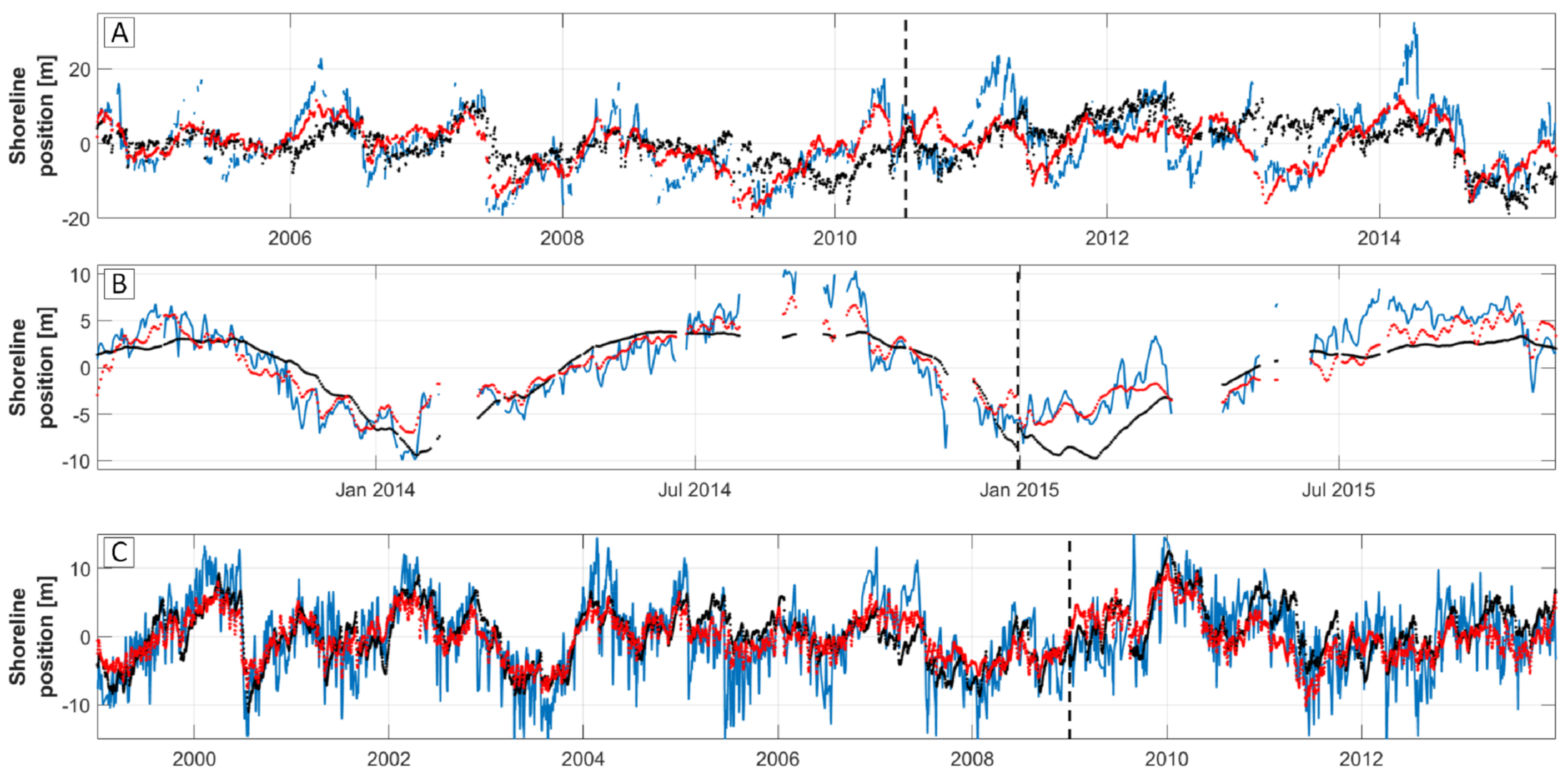
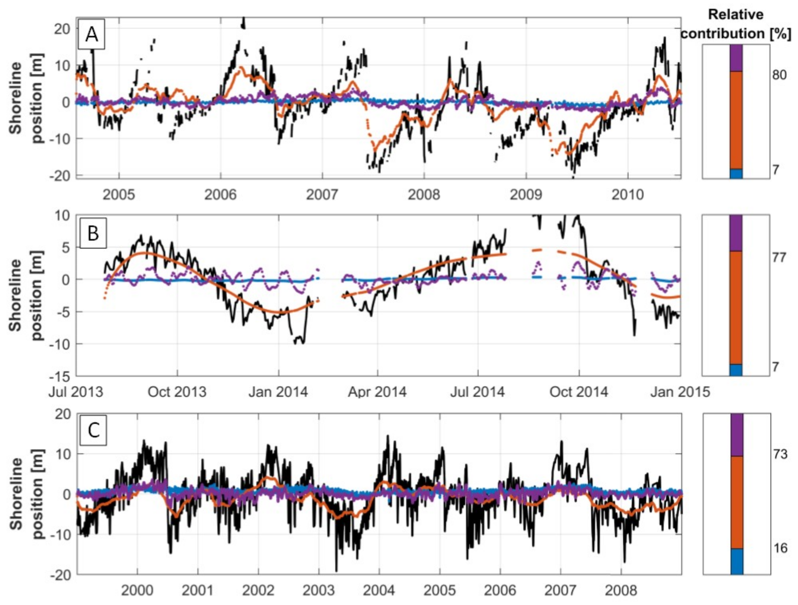
Figure 5 presents the results (calibration and validation) when SF-ST (black) and SF-MT (red) are applied to the datasets at Narrabeen (Figure 5A), Nha Trang (Figure 5B) and Tairua (Figure 5C). The transition between the calibration and validation time periods is indicated with a dashed black line. Figure 6 presents the contribution of each model improvement step over time (left, in similar order) and the corresponding relative contribution of each model improvement step (right) for the calibration period only. The blue, orange and purple lines correspond to the direct forcing, upscaling and downscaling approaches, respectively. In Figure 7 the standard deviation per timescale cluster is shown (left panels) for the shoreline position data (green), the SF-ST (black) and SF-MT (red) model result (calibration + validation) for all datasets (in similar order as Figure 5 and Figure 6). Note that, to show the standard deviation per timescale cluster for SF-ST, the filter function is applied to the SF-ST model result. In the middle panel, the correlation between the SF-MT model result (and SF-ST) and the shoreline position data is presented on all different timescales. In the right panels, a model score is given for each of the three model improvement steps for all different timescales. The score for every timescale consists of the correlation coefficient (model result—data on that particular timescale) multiplied by standard deviation of that modelled signal, timescale and model improvement step. Using this modelling result score means that (1) if the correlation between the data model is high, the model is able to reproduce shoreline change at this timescale, (2) if the standard deviation of the model result is high, that particular shoreline signal is important in determining shoreline change according to Equation (4).

For the Narrabeen dataset (Figure 5A) SF-ST (black) is able to capture the smaller timescale storm/swell response (order of days), but the larger timescale shoreline variations are captured to a lesser extent (φ = 3 days and c = 1.96 × 10⁻⁷ (m/s)/(W/m)^0.5). The SF-MT model (red) also captures the storm timescale to a certain extent, but yields a considerable increase in skill (BSS of 0.61 or an ‘excellent’ rating) by better capturing shoreline change on larger timescales (larger than the storm timescale). This occurs, for example, in 2009, where first the large erosion period halfway through 2009 is captured well by the SF-MT model and poorly by SF-ST, while the same occurs for the accretive period during the second half of 2009. Regarding the energetic storm sequence in June 2007 (see Section 2), neither model is capable of capturing the rapid shoreline recession. Overall, the SF-MT model yields a better fit to the data, compared to SF-ST, which seems to underestimate the amplitude of shoreline accretion/erosion most of the time. This is emphasized by the NMS error between the data and model result, which is 0.71 for SF-ST and reduces to 0.29 for the SF-MT model. This corresponds to a ‘fair’ and ‘excellent’ rating for SF-ST and SF-MT, respectively. The correlation coefficient is substantially larger for SF-MT as well (63%). The standard deviation and correlation plot per timescale (Figure 7A) shows that for storm/swell timescales (1–12 days) SF-ST has a higher standard deviation and a similar correlation. Hence, the smaller storm timescales are better captured by the SF-ST model. However, for SF-MT the standard deviation multiplied with the correlation is higher for timescales larger than 33 days (up to 2285 days). Hence, the dominant seasonal timescale is better captured by the SF-MT model, which contributes most to the model improvement. Moreover, the upscaling approach contributes considerably (73%) to the total shoreline signal (orange line in Figure 6A). The larger timescales are captured by the upscaling and downscaling (purple, Figure 7A) approaches whereas the smaller (storm/swell) timescales are captured by the downscaling approach as well. The direct forcing approach (blue) has a limited contribution to the total model result (7%, Figure 6A), compared to the upscaling (73%) and downscaling (20%) approach. The ∆AIC score (difference in AIC score between SF-ST and SF-MT) is larger than 1, which indicates that a considerable model improvement is acquired during the calibration phase.

At Nha Trang considerable improvement is made by implementing multiple timescales within the SF-ST model (Figure 5B), which is emphasized by a BSS of 0.62 (i.e., an ‘excellent’ rating). Where SF-ST (φ = 180 days and c = 4.61 × 10⁻⁸ (m/s)/(W/m)^0.5) only partially captures the seasonal timescale (the most dominant timescale, see Table 2 and Figure A1), the SF-MT model captures both the response to monsoons and the seasonal variation in wave data (i.e., the two dominant timescales in the wave data). The response to the energetic typhoon in November 2013 is not captured by SF-ST nor SF-MT. The NMS errors for SF-ST and SF-MT with the data is 0.31 (‘good’) and 0.13 (‘excellent’), respectively. Figure 7B shows that the standard deviation and correlation per timescale for SF-MT (red) are high and relatively uniformly distributed across the different timescales. This states that all timescales are well captured (except for the typhoons with a daily timescale). For SF-ST (black) the correlation is lower for all timescales except for the seasonal variation, where the correlation is similar. The standard deviation is lower/higher for timescales smaller/larger than 78 days. If both indicators are combined, it becomes clear that the largest contributor to the model improvement of SF-MT are the smaller timescales (i.e., the monsoons). Furthermore, note that an improvement is already made by using the upscaling approach only (orange line Figure 6B). However, in that case, only the response to the seasonal variation is captured. The response to monsoons (timescale of ≈ 20 days) is captured by the downscaling approach (purple). The relative contribution of each model improvement step indicates as well that the seasonal timescale (upscaling) is the most dominant (70%) in determining coastline evolution, followed by the monsoon response (downscaling, 23%). Figure 7B implies as well that the downscaling approach captures the smaller timescales (monsoons), while the larger timescales (seasonal variation) are captured by the upscaling approach. The ∆AIC score is larger than 1, which implicates that the larger number of calibration parameters in the SF-MT model is justified by a considerably better model fit (relative to SF-ST).

From Figure 5C it becomes clear that the SF-ST (black, φ = 150 days and c = 1.03 × 10⁻⁷ (m/s)/(W/m)^0.5) and SF-MT (red) model both capture shoreline change well for the dataset at Tairua and at first sight model differences are less pronounced than for the dataset at Narrabeen and Nha Trang. The NMS error indicates that there are differences: 0.51 for SF-ST and 0.36 for SF-MT. However, they both correspond to a ‘good’ rating, although the error is considerably lower for SF-MT. This difference is also emphasized by the BSS of 0.3, indicating that SF-MT is a ‘good’ improvement compared to SF-ST. The better model capability of SF-MT to capture shoreline change is emphasized as well in Figure 7C: both the standard deviation and the correlation for storm to monthly dominant timescales are higher for SF-MT. Those figures show as well that for the dominant seasonal to inter-annual timescales shoreline change is captured well by both models. However, there are certain moments in time where the SF-MT model outperforms SF-ST. This occurs, for example, at the end of 2006/beginning of 2007, where the accretion period is not well captured by SF-ST (Figure 5C). The rapid response to the series of huge storms that occurred in the winter of 2000 is captured reasonably by both models. From Figure 6C and Figure 7C becomes clear that the larger dominant seasonal to inter-annual timescales are modelled using the upscaling approach (orange, 57%), the smaller timescales are modelled using the downscaling (monthly timescale, purple, 27%) and direct forcing approach (storm/swell timescale, blue, 16%). Moreover, the ∆AIC score is larger than 1, which indicates that a considerable model improvement is acquired. Note that the correlation coefficient is higher for SF-MT as well (0.85 compared to 0.70 for SF-ST).

4.2. Validation

During model validation, wave data in combination with the calibrated free parameters found in Section 4.1 are used to predict shoreline evolution. However, measured shoreline data is still available and is used to compare with the shoreline predictions.

For the validation phase, shoreline predictions are shown in Figure 5 as well.

The validation results at Narrabeen reveal that the result of SF-MT outperforms that of SF-ST, but differences are less pronounced as for the calibration phase (BSS of 0.26 or a ‘good’ rating, compared to 0.61 or an ‘excellent’ rating for the calibration phase). From the timeseries in Figure 5A, it becomes clear that especially after 2013, the prediction of SF-MT is closer to the data than the prediction of SF-ST. The NMS error between the data and model prediction is 0.83 for the SF-ST model, which reduces to 0.61 for the SF-MT model. This corresponds to a ‘poor’ and ‘fair’ rating, respectively. The overall variability of the beach is better represented by the SF-MT model, which is emphasized by the correlation coefficient (0.45 compared to 0.62, for SF-ST and SF-MT, respectively). The ∆AIC score is smaller than 1. This indicates that SF-ST is preferred according to this score, due to the trade-off between the model’s simplicity and goodness of fit. The ∆AIC score indicates that for the SF-MT model the number of calibration parameters (i.e., decreased model simplicity), which is penalized for by the AIC score (Equation (A7)), is too large compared to the goodness of fit (relative to SF-ST).

The model validation phase at Nha Trang shows similar characteristics as for the calibration phase as the seasonal variation and the response to summer and winter monsoons are well predicted by SF-MT, while the SF-ST model only partially captures the seasonal variation (Figure 5B). The NMS error for SF-ST and the SF-MT model is 0.63 and 0.26, which corresponds to a ‘fair’ and ‘excellent’ rating, respectively. The similar characteristics for the calibration and validation phase are also emphasized by the BSS, which is 0.61 for the validation phase while it was 0.62 for the calibration phase (i.e., an ‘excellent’ rating). The ∆AIC score is smaller than 1, which indicates that the SF-ST model is preferred due to the model’s simplicity compared to the relative goodness of fit.

A comparison of the validation results for both models at Tairua (Figure 5C) shows that some improvement is made by implementing multiple timescales in SF-ST, especially during the last 2 to 3 years of the dataset (BSS of 0.18 or a ‘fair’ model improvement). Overall, the SF-MT model predicts shoreline change better than SF-ST, which results in a decrease in the NMS error of 18% and an increase in the correlation coefficient of 8% (

Table 3. Model skill during the calibration and validation phase, for the SF-ST and SF-MT model, at all three sites, using four model skill indicators.

Site	Indicator	Calibration			Validation
		SF-ST	SF-MT	%	SF-ST	SF-MT	%
Narrabeen	R	0.52	0.85	63	0.45	0.62	38
	NMSE	0.71	0.29	−59	0.83	0.61	−27
	BSS	-	0.61	-	-	0.26	-
	∆AIC	-	>1	-	-	<1	-
Nha Trang	R	0.83	0.94	13	0.86	0.89	3
	NMSE	0.31	0.13	−58	0.63	0.26	−59
	BSS	-	0.62	-	-	0.61	-
	∆AIC	-	>1	-	-	<1	-
Tairua	R	0.70	0.85	21	0.60	0.65	8
	NMSE	0.51	0.36	−29	0.71	0.58	−18
	BSS	-	0.3	-	-	0.18	-
	∆AIC	-	>1	-	-	<1	-

). The rating of the NMS error for SF-ST and SF-MT is ‘fair’ and ‘good’, respectively. The ∆AIC score is smaller than 1, which indicates that the SF-ST model is preferred due to the model’s simplicity compared to the relative goodness of fit.

5. Discussion

This work was motivated by the fact that single memory decay models fail to reproduce shoreline evolution at sites where multiple forcing timescales are present, such as seasonal and monsoon forcing. In this paper, we focused on a single memory decay hybrid model that predicts temporal changes of the shoreline location due to varying wave conditions. Although there are hybrid models that account for shoreline change due to, for example, cross-shore processes, longshore processes, sea level rise and include the beach-dune system [21,46,47,48], here the focus was on shoreline changes due to cross-shore and wave induced processes only. The hybrid model used here as a base is the ShoreFor model (SF-ST; Shoreline Forecast—Single Timescale—see description in Appendix A), by [17]. This model uses a holistic understanding of how a beach responds to several high-intensity forcing event characteristics (duration, intensity, clustering and recovery, see Section 1), but model skill deteriorates considerably if multiple dominant forcing and beach response timescales are present. The Shoreline Forecast Multiple Timescales (SF-MT) model basically uses the same holistic understanding as SF-ST of how a beach responds to wave forcing. However, it is not optimized once for the raw wave and shoreline position timeseries, but multiple times for each timescale separately (including upscaling and downscaling procedures). In [49], an extensive research about the behavior and structure of the SF-ST model was performed, where it was shown and confirmed that within SF-ST the shoreline change is solely dependent on the past and present wave conditions, the SF-ST model mainly has one characteristic timescale and the model has a sort of implicit damping timescale introduced by φ in Equation (A4). Hence, it is possible to create a model for multiple timescales, based on SF-ST, that represents a sum of individual components (i.e., timescale clusters) from several equilibrium shoreline models with different timescales.

In [50], a different approach to model multiple timescales (from storm events to decadal time-scales) was developed (based on the Complete Ensemble Empirical Mode Decomposition method), and applied to the Narrabeen and Tairua dataset. Their approach first identifies and subsequently links the primary timescales in the large-scale sea level pressure and/or waves with identical timescales in the shoreline position (i.e., a direct forcing approach). Intriguingly, they found similar results as presented in this paper. For Narrabeen they found timescales of 181, 363 and 709 days to be important shoreline position timescales (besides the long-term trend). Other timescales of 17, 45, 85 and 1291 days were important as well, but showed less shoreline variability. Here, Figure 7A shows a high standard deviation and correlation (and thus high shoreline variability) of the SF-MT shoreline prediction for timescales of approximately 52, 98, 184, 368, 528, 752 and 1900 days. For Tairua [50] found timescales of 980, 146 and 352 days to be important shoreline variability timescales, and to a lesser extent timescales of 15, 39, 73, 1125, 1911 and 4537 days. The SF-MT model showed similar results here (although to a lesser extent compared to Narrabeen), where Figure 7C shows that the important shoreline variability timescales (high correlation and standard deviation) are approximately all timescale clusters between 236 and 1962 days and 14 days. Hence, good agreement with results from a different multi-timescale model is achieved.

Apart from an increase in model prediction skill (Table 3), compared to SF-ST, the SF-MT model also gains insight in how a beach responds to the considered wave forcing on multiple scales. The contribution of each model improvement step to shoreline evolution (Figure 6 and Figure 7) illustrates, for example, that at all sites’ extreme forcing events have a considerable and persistent shoreline impact (i.e., upscaling approach). It showed that these forcing events are responsible for 57 to 73% of the variability of shoreline evolution. Moreover, at all study sites long-term shoreline trends affect short-term forcing event impacts (i.e., downscaling approach). These affected short-term forcing event impacts are responsible for 20 to 27% of the variability of shoreline evolution. Moreover, the distribution of shoreline variability over the different modelling approaches and timescale clusters in SF-MT (last column in Figure 7), showed that the upscaling approach is responsible for capturing shoreline change on the largest timescales in the dataset, which is logical, as this approach is modelling the persistent effect of short high-intensity wave forcing events on larger shoreline response timescales. Conversely, the modelled shorelines generated with the downscaling approach correspond better to shoreline data on smaller timescales, which is logical as well, as this approach is modelling the effect of the larger timescales in shoreline variation on the efficiency with which smaller timescale wave forcing events induce cross-shore sediment transport. The direct forcing approach does not account for particular shoreline response timescales as it seems to be dataset dependent.

Besides the literature mentioned in Section 2, the temporal spectra (Section 3.1 and Figure A1) reveal the presence of multiple dominant timescales. These spectra can be considered before model application and can be used to determine if the SF-MT model is more favorable to use with respect to SF-ST (considering model complexity): multiple dominant forcing timescales lead to a substantial improvement (e.g., Narrabeen and Nha Trang, BSS of 0.61 and 0.62, respectively), while if a single timescale is present, a less substantial improvement can be expected (Tairua, BSS of 0.30). For all study sites, the ∆AIC score is larger than 1 for the calibration phase, indicating a considerable model improvement is acquired when accounting for model skill and complexity. However, for the validation phase the ∆AIC score is smaller than 1. In the case of a low/negative ∆AIC score and a limited number of observed dominant timescales, a reduced number of bins can also be tested to increase the ∆AIC score. Nevertheless, SF-MT currently handles a large number of ‘blind’ bins by giving low/no weight to timescale clusters where low variability is observed to have an unbiased result regarding timescale interactions (rather than hardwire on dominant timescales before model application). The multi-timescale model outperforms SF-ST at sites where short-term (2–3 years) and long-term (10–14 years) data is available. Interestingly, for longer period simulations, climate variability induces changes in wave regimes at all scales, storminess of storm tracks in mid-latitudes, tropical cyclones, but also monsoons and seasonal to inter-annual average conditions [21,51]. Moreover, as a variable climate is expected, multiple timescales of shoreline adjustment to forcing likely exist almost everywhere. In that context, the humble simplified approach developed in SF-MT can be an attractive way to capture shoreline change to climate modes, climate change and their timescale-interactions.

Although the SF-MT model outperforms SF-ST at three hydrodynamic and morphologically dissimilar sites, it is far from a perfect shoreline prediction model as it still does not capture a large part of the observed shoreline variability, which can have several reasons:

• Although camera-derived shorelines give a shoreline proxy, instantaneous and/or time averaged imagery is going to be affected by the role of tidal fluctuations, sea level anomalies and wave run-up. Moreover, sediments can be built up as a berm above the mean high water line and may not show up at all when using a single contour for the shoreline location. All those mechanisms/effects can have an influence on the shoreline location and are not accounted for in the model.
• Due to the linear interpolation of the shoreline location (for Nha Trang) and wave forcing parameters (i.e., H_s and T_p) for all study sites to a single value uniformly spaced every 24 h apart, information is lost, which could induce errors when predicting shoreline change (e.g., storm and tidal aliasing effects). This data handling has a larger effect on the storm timescales compared to seasonal and inter-annual timescales (which were generally captured well by the model). Figure 7 shows that sub-weekly timescales are captured to a lesser extent compared to larger timescales (small standard deviation and correlation). Moreover, at these smaller timescales detailed morphodynamics can become critical for beach response, but they are not incorporated in SF-MT, and besides that, the equilibrium concept is at its limit for those small timescales. All these effects can be the cause for the relatively bad prediction skill for sub-weekly timescales. This is emphasized by the fact that the rapid response to the energetic (series of) storms, highlighted in Section 2, was not captured well by both models at Narrabeen and Nha Trang (and fairly reasonable at Tairua).
• A second-order polynomial was used to detrend the raw shoreline position timeseries to remove timescales which are larger than the length of the dataset. However, it is possible that there is a relation between this second-order polynomial trend and how the beach responds to incoming wave forcing. For example, a strong erosive trend throughout the timeframe of the dataset would mean that the impact of monsoons become less as time progresses. This phenomenon is not implemented in SF-MT.
• As all study sites comprise embayed beaches, it is possible that longshore effects play a role due to, for example, long-term rotation of the beach, whereas the current model only accounts for cross-shore processes. At Narrabeen and Nha Trang, this mechanism is minimized to a certain extent as the shoreline location was determined by longshore averaging a certain stretch of the beach which is close to the center of rotation. Moreover, there could be an effect on the shoreline location of the angle of wave incidence (or sea level pressure variations as was shown by [50]) as it may also vary on different timescales. Those phenomena are not implemented in the model.

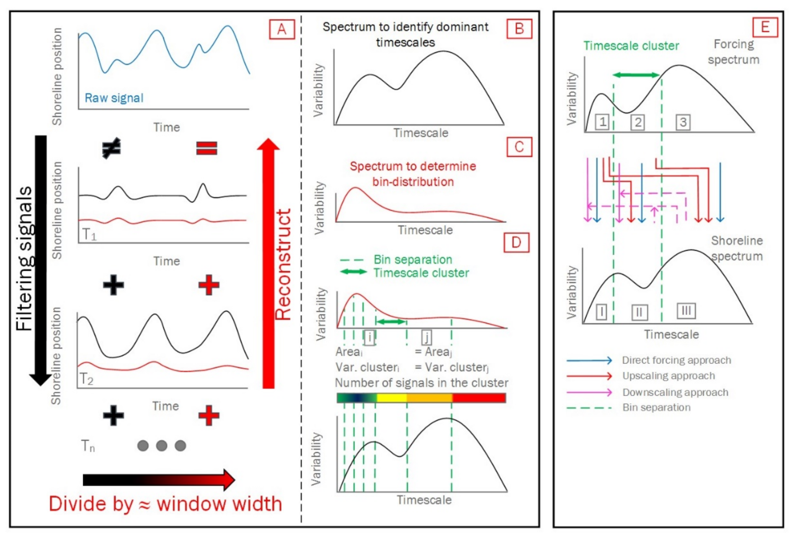
Timescale Interactions

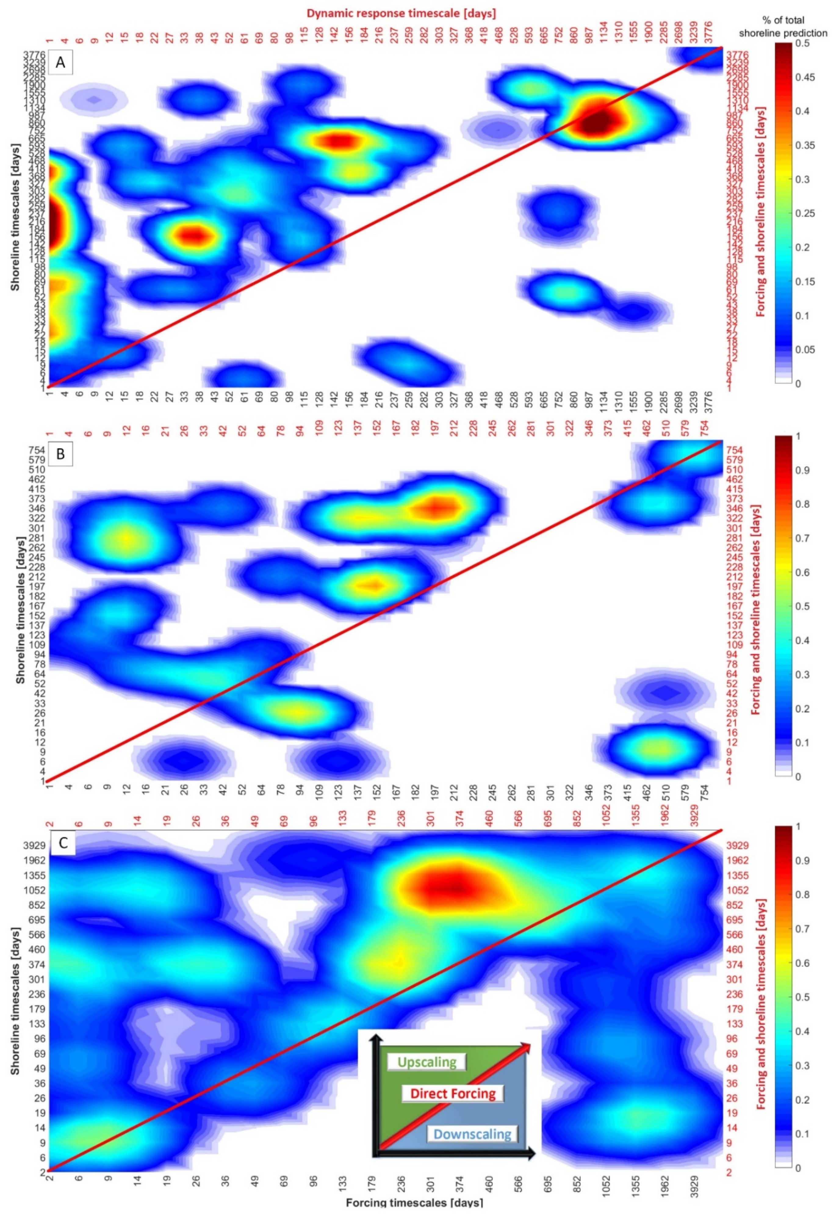
The SF-MT model generates multiple individual signals, in which each signal (i.e., timescale cluster) has a unique timescale relation between the wave forcing and shoreline signal. A certain selection of all these generated signals make up the total shoreline signal (Section 3.3, Equation (4)). To visualize these unique timescale relations of all chosen modelled signals, a grid of timescale interactions is presented (Figure 8). In those grids, the percentage to the total shoreline signal per individual modelled signal (i.e., timescale cluster) is plotted, revealing the most important timescale interactions per dataset. The axes can be used to check which timescales are considered and the diagonal, upper left corner and lower right corner correspond to signals generated with the direct forcing, upscaling, and downscaling approach, respectively. Figure 8 presents the timescale interactions at Narrabeen (Figure 8A), Nha Trang (Figure 8B) and Tairua (Figure 8C).

The interactions between timescales shown in Figure 8A show that at Narrabeen the short-term high-intensity forcing events with a timescale of approximately 1 to 6 days have a large and persistent impact on the large timescale shoreline variation (quasi-seasonal). Moreover, shoreline variability on inter-annual timescales is driven by variations in the wave climate with a similar timescale, but it is sensitive to whether the coastline is eroded or accreted on a mildly larger timescale of approximately 860–1134 days (i.e., downscaling approach). This means that the impact to inter-annual forcing events is dependent on whether that coastline is eroded or accreted on a similar to larger timescale.

In contrast, Figure 8B shows that at Nha Trang small(er) timescales in the wave forcing (especially those with a timescale of 123–197 days) have a persistent and considerable effect on coastline evolution, and which is together with the persistent effect of monsoons the cause of the seasonal variability (i.e., upscaling). Furthermore, as indicated by the timeseries in Figure 6B, shoreline response to both summer and winter monsoons is affected by longer-term shoreline variations (i.e., downscaling). This means that the response to these monsoons is not equal throughout the year. Beach response to monsoons (with a timescale of approximately 10–30 days) is larger when the shoreline is already accreted on a larger timescale (3 months or 1.5 year, see Figure 8B). This supports the fact that due to an overall accreted beach state, the sand supply from within the surf zone is close to the shoreline, which yields a high sediment transport efficiency and faster response to monsoons. Conversely, when the coastline is already eroded on a larger timescale, the monsoon response is relatively smaller: a large spatial separation between the shoreline and the more offshore sediment source yields an inefficient transfer of sediment between the more offshore region and beach face, causing a lower response rate.

Figure 8C visualizes the timescale interactions at Tairua. It shows that the wave forcing with an annual timescale has a large and persistent impact on the inter-annual shoreline response (852–1355 days). Moreover, shoreline response on the smallest (storm/swell) timescales (6–9 days) is driven by wave forcing events on a similar timescale (i.e., direct forcing). Furthermore, the inter-annual shoreline change (i.e., timescales of 1052 to 1355 days) has an influence on how the beach responds to the short timescale wave forcing events with a timescale of approximately 9 to 19 days (i.e., downscaling).

6. Conclusions

In this study, a new approach is presented to allow for multiple wave forcing and beach response timescales within the single-timescale equilibrium shoreline prediction model ShoreFor (SF-ST; Shoreline Forecast—Single Timescale). While SF-ST was only capable of accurately predicting shoreline change on the single most dominant beach response timescale, multiple dominant timescales can determine shoreline evolution. The multi-timescale implementation (SF-MT; Shoreline Forecast—Multiple Timescales) is governed by filtering and identifying all of the wave forcing and shoreline response timescales. Subsequently, timescales in the wave forcing and shoreline signals are linked through a direct forcing term (as used in SF-ST) and two additional terms: a time-upscaling and a time-downscaling term. In the direct forcing term, the shoreline is forced by waves on the corresponding timescales (e.g., a beach erodes and recovers to an individual storm). The upscaling term accounts for the persistent effect of short(er) forcing timescales on longer shoreline response timescales (e.g., seasonal persistence of summer and winter monsoons). This is modelled using the envelope of the filtered wave signals, which provides the timescale link. The downscaling approach governs the effect of long(er) timescales of shoreline evolution on shoreline response to short(er) wave forcing timescales (e.g., storm impact during accreting or eroding trends). This effect is modelled by introducing a time-dependent response factor from a filtered longer timescale shoreline evolution signal. The multi-timescale model showed improvement compared to SF-ST at the three sandy, microtidal, but hydrodynamic and morphologically contrasted sites used in this study: the normalized mean square error was improved during validation by 27, 59 and 18% for Narrabeen, Nha Trang and Tairua, respectively. In the case of multiple dominant forcing timescales, a substantial improvement is achieved (i.e., Narrabeen and Nha Trang), otherwise improvement is less substantial (i.e., Tairua). For all sites, we found that extreme forcing events have a considerable and persistent shoreline impact (i.e., upscaling term, responsible for 57 to 73% of the variability of shoreline evolution). This effect was the most pronounced at Narrabeen, where short-term high-intensity forcing events with a timescale of approximately 1 to 6 days have a large and persistent impact on the quasi-seasonal shoreline evolution. Moreover, at all study sites long-term shoreline trends affect short-term forcing event impacts (i.e., downscaling term, responsible for 20 to 27% of the variability of shoreline evolution). This effect was the most striking at Nha Trang, where we showed that shoreline response to both summer and winter monsoons is affected by longer-term shoreline variations: in the case of an overall accreted (eroded) beach state, the sand supply from within the surf zone is close to (far from) the shoreline, which yields a high (low) sediment transport efficiency and faster (slower) response to monsoons. Dealing with multiple timescales and their interactions, this combined approach leads to several interests when considering interplay between climate modes and storminess under climate change when forecasting future shoreline evolution.

References

1. Larson, M.; Kraus, N.C. Prediction of cross-shore sediment transport at different spatial and temporal scales. Mar. Geol. 1995, 126, 111–127. [Google Scholar] [CrossRef]
2. Pianca, C.; Holman, R.; Siegle, E. Shoreline variability from days to decades: Results of long-term video imaging. J. Geophys. Res. Ocean. 2015, 120, 2159–2178. [Google Scholar] [CrossRef]
3. Almar, R.; Marchesiello, P.; Almeida, L.P.; Thuan, D.H.; Tanaka, H.; Viet, N.T. Shoreline response to a sequence of typhoon and monsoon events. Water 2017, 9, 364. [Google Scholar] [CrossRef] [Green Version]
4. Plant, N.G.; Aarninkhof, S.G.J.; Turner, I.L.; Kingston, K.S. The Performance of Shoreline Detection Models Applied to Video Imagery. J. Coast. Res. 2007, 233, 658–670. [Google Scholar] [CrossRef]
5. Bergsma, E.; Almar, R. Coastal coverage of ESA’ Sentinel 2 mission. Adv. Space Res. 2020, 65, 2636–2644. [Google Scholar] [CrossRef]
6. Montaño, J.; Coco, G.; Antolínez, J.A.A.; Beuzen, T.; Bryan, K.R.; Cagigal, L.; Castelle, B.; Davidson, M.A.; Goldstein, E.B.; Ibaceta, R.; et al. Blind testing of shoreline evolution models. Sci. Rep. 2020, 10, 2137. [Google Scholar] [CrossRef] [PubMed] [Green Version]
7. Ibaceta, R.; Splinter, K.D.; Harley, M.D.; Turner, I.L. Enhanced Coastal Shoreline Modeling Using an Ensemble Kalman Filter to Include Nonstationarity in Future Wave Climates. Geophys. Res. Lett. 2020, 47. [Google Scholar] [CrossRef]
8. Walstra, D.J.R.; Reniers, A.J.H.M.; Ranasinghe, R.; Roelvink, J.A.; Ruessink, B.G. On bar growth and decay during inter-annual net offshore migration. Coast. Eng. 2012, 60, 190–200. [Google Scholar] [CrossRef]
9. Walstra, D.J.R.; Wesselman, D.A.; van der Deijl, E.C.; Ruessink, G. On the Intersite Variability in Inter-Annual Nearshore Sandbar Cycles. Mar. Sci. Eng. 2016, 4, 15. [Google Scholar] [CrossRef] [Green Version]
10. Callaghan, D.P.; Ranasinghe, R.; Roelvink, D. Probabilistic estimation of storm erosion using analytical, semi-empirical, and process based storm erosion models. Coast. Eng. 2013, 82, 64–75. [Google Scholar] [CrossRef]
11. Roelvink, D.; Reniers, A.; van Dongeren, A.; van Thiel de Vries, J.; McCall, R.; Lescinski, J. Modelling storm impacts on beaches, dunes and barrier islands. Coast. Eng. 2009, 56, 1133–1152. [Google Scholar] [CrossRef]
12. Bruun, P. Coast. Erosion and the Development of Beach Profiles; US Beach Erosion Board: Washington, DC, USA, 1954; Volume 44. [Google Scholar]
13. Dean, R.G. Equilibrium Beach Profiles: US Atlantic and Gulf Coasts; Department of Civil Engineering and College of Marine Studies, Newark, University of Delaware: Newark, DE, USA, 1977. [Google Scholar]
14. Goldstein, E.B.; Coco, G.; Plant, N.G. A review of machine learning applications to coastal sediment transport and morphodynamics. Earth-Sci. Rev. 2019, 194, 97–108. [Google Scholar] [CrossRef] [Green Version]
15. Miller, J.K.; Dean, R.G. A simple new shoreline change model. Coast. Eng. 2004, 51, 531–556. [Google Scholar] [CrossRef]
16. Yates, M.L.; Guza, R.T.; O’Reilly, W.C. Equilibrium shoreline response: Observations and modeling. J. Geophys. Res. 2009, 114. [Google Scholar] [CrossRef] [Green Version]
17. Davidson, M.A.; Splinter, K.D.; Turner, I.L. A simple equilibrium model for predicting shoreline change. Coast. Eng. 2013, 73, 191–202. [Google Scholar] [CrossRef]
18. Splinter, K.D.; Turner, I.L.; Davidson, M.A.; Patrick, B.; Castelle, B.; Oltman–Shay, J. A generalized equilibrium model for predicting daily to interannual shoreline response. Geophys. Res. Earth Surf. 2014, 119, 1936–1958. [Google Scholar] [CrossRef] [Green Version]
19. Splinter, K.D.; Turner, I.; Reinhardt, M.; Ruessink, B. Rapid adjustment of shoreline behaviour to changing seasonality of storms: Observations and modelling at an open-coast beach. Earth Surf. Process. Landf. 2017, 42, 1186–1194. [Google Scholar] [CrossRef]
20. Splinter, K.D.; Turner, I.L.; Davidson, M.A. How much data is enough? The importance of morphological sampling interval and duration for calibration of empirical shoreline models. Coast. Eng. 2013, 77, 14–27. [Google Scholar] [CrossRef]
21. Vitousek, S.; Barnard, P.L.; Limber, P.; Erikson, L.; Cole, B. A model integrating longshore and cross-shore processes for predicting long-term shoreline response to climate change. J. Geophys. Res. Earth Surf. 2017, 122, 782–806. [Google Scholar] [CrossRef]
22. Angnuureng, D.B.; Almar, R.; Senechal, N.; Castelle, B.; Addo, K.A.; Marieu, V.; Ranasinghe, R. Shoreline resilience to individual storms and storm clusters on a meso-macrotidal barred beach. Geomorphology 2017, 290, 265–276. [Google Scholar] [CrossRef]
23. Karunarathna, H.; Pender, D.; Ranasinghe, R.; Short, A.D.; Reeve, D.E. The effects of storm clustering on beach profile variability. Mar. Geol. 2014, 348, 103–112. [Google Scholar] [CrossRef] [Green Version]
24. Morton, R.A.; Paine, J.G.; Gibeaut, J.C. Stages and durations of post-storm beach recovery, southeastern Texas Coast, U.S.A. J. Coast. Res. 1994, 10, 884–908. [Google Scholar]
25. Dodet, G.; Castelle, B.; Masselink, G.; Scott, T.; Davidson, M.; Floc’h, F.; Jackson, D.; Suanez, S. Beach recovery from extreme storm activity during the 2013-14 winter along the Atlantic coast of Europe. Earth Surf. Process. Landf. 2019, 44, 393–401. [Google Scholar] [CrossRef] [Green Version]
26. Frazer, L.N.; Anderson, T.R.; Fletcher, C.H. Modeling storms improves estimates of long-term shoreline change. Geophys. Res. Lett. 2009, 36. [Google Scholar] [CrossRef] [Green Version]
27. Anderson, T.R.; Frazer, L.N.; Fletcher, C.H. Transient and persistent shoreline change from a storm. Geophys. Res. Lett. 2010, 37. [Google Scholar] [CrossRef] [Green Version]
28. Long, J.W.; Plant, N.G. Extended Kalman Filter framework for forecasting shoreline evolution. Geophys. Res. Lett. 2012, 39, L13603. [Google Scholar] [CrossRef]
29. Bergsma, E.; Conley, D.; Davidson, M.; O’Hare, T.; Almar, R. Storm Event to Seasonal Evolution of Nearshore Bathymetry Derived from Shore-Based Video Imagery. Remote Sens. 2019, 11, 519. [Google Scholar] [CrossRef] [Green Version]
30. Thuan, D.H.; Almar, R.; Marchesiello, P.; Viet, N. Video Sensing of Nearshore Bathymetry Evolution with Error Estimate. J. Mar. Sci. Eng. 2019, 7, 233. [Google Scholar] [CrossRef] [Green Version]
31. Holman, R.A.; Stanley, J. The history and technical capabilities of Argus. Coast. Eng. 2007, 54, 477–491. [Google Scholar] [CrossRef]
32. Ondoa, G.A.; Almar, R.; Jouanno, J.; Bonou, F.; Castelle, B.; Larson, M. Beach adaptation to intraseasonal sea level changes. Environ. Res. Commun. 2020, 2, 051003. [Google Scholar] [CrossRef]
33. Phillips, M.S.; Harley, M.D.; Turner, I.L.; Splinter, K.D.; Cox, R.J. Shoreline recovery on wave-dominated sandy coastlines: The role of sandbar morphodynamics and nearshore wave parameters. Mar. Geol. 2017, 385, 146–159. [Google Scholar] [CrossRef]
34. Harley, M.D.; Turner, I.; Short, A.; Ranasinghe, R. A reevaluation of coastal embayment rotation: The dominance of cross-shore versus alongshore sediment transport processes in SE Australia. J. Geophys. Res. 2011, 116. [Google Scholar] [CrossRef]
35. Blossier, B.; Bryan, K.R.; Daly, C.J.; Winter, C. Shore and bar cross-shore migration, rotation, and breathing processes at an embayed beach. J. Geophys. Res. Earth Surf. 2017, 122, 1745–1770. [Google Scholar] [CrossRef]
36. Bradshaw, B.; Healy, T.R.; Dell, P.M.; Bolstad, W. Inner Shelf Dynamics on a Storm-Dominated Coast, East Coromandel, New Zealand. J. Coast. Res. 1991, 7, 11–30. [Google Scholar]
37. Turner, I.L.; Harley, M.D.; Short, A.D.; Simmons, J.A.; Bracs, M.A.; Phillips, M.S.; Splinter, K.D. A multi-decade dataset of monthly beach profile surveys and inshore wave forcing at Narrabeen, Australia. Sci. Data 2016, 3. [Google Scholar] [CrossRef] [Green Version]
38. Davidson, M.A.; Splinter, K.D.; Turner, I.L.; Harley, M.D. Annual prediction of shoreline erosion and subsequent recovery. Coast. Eng. 2017, 130, 14–25. [Google Scholar] [CrossRef] [Green Version]
39. Ranasinghe, R.; McLoughlin, R.; Short, A.; Symonds, G. The Southern Oscillation Index, wave climate, and beach rotation. Mar. Geol. 2004, 204, 273–287. [Google Scholar] [CrossRef]
40. Harley, M.D.; Turner, I.L.; Short, A.D.; Ranasinghe, R. Interannual variability and controls of the Sydney wave climate. Int. J. Climatol. 2010, 30, 1322–1335. [Google Scholar] [CrossRef]
41. Lefebvre, J.P.; Almar, R.; Viet, N.T.; Thuan, D.H.; Binh, L.T.; Ibaceta, R.; Duc, N.V. Contribution of swash processes generated by low energy wind waves in the recovery of a beach impacted by extreme events: Nha Trang, Vietnam. J. Coast. Res. 2014, 70, 663–668. [Google Scholar] [CrossRef]
42. Thuan, D.H.; Binh, L.T.; Viet, N.T.; Hanh, D.K.; Almar, R.; Marchesiello, P. Typhoon impact and recovery from continuous video monitoring: A case study from Nha Trang Beach, Vietnam. J. Coast. Res. 2016, 75, 263–267. [Google Scholar] [CrossRef]
43. Smith, R.K.; Bryan, K.R. Monitoring Beach Face Volume with a Combination of Intermittent Profiling and Video Imagery. J. Coast. Res. 2007, 234, 892–898. [Google Scholar] [CrossRef]
44. van de Lageweg, W.; Bryan, K.; Coco, G.; Ruessink, B. Observations of shoreline–sandbar coupling on an embayed beach. Mar. Geol. 2013, 344, 101–114. [Google Scholar] [CrossRef]
45. Aagaard, T.; Kroon, A.; Andersen, S.; Sørensen, R.M.; Quartel, S.; Vinther, N. Intertidal beach change during storm conditions; Egmond, the Netherlands. Mar. Geol. 2005, 218, 65–80. [Google Scholar] [CrossRef]
46. Antolínez, J.A.A.; Méndez, F.J.; Anderson, D.; Ruggiero, P.; Kaminsky, G.M. Predicting Climate-Driven Coastlines with a Simple and Efficient Multiscale Model. J. Geophys. Res. Earth Surf. 2019, 124, 1596–1624. [Google Scholar] [CrossRef] [Green Version]
47. Robinet, A.; Idier, D.; Castelle, B.; Marieu, V. A reduced-complexity shoreline change model combining longshore and cross-shore processes: The LX-Shore model. Environ. Model. Softw. 2018, 109, 1–16. [Google Scholar] [CrossRef]
48. Robinet, A.; Castelle, B.; Idier, D.; Harley, M.; Splinter, K. Controls of local geology and cross-shore/longshore processes on embayed beach shoreline variability. Mar. Geol. 2020, 422, 106118. [Google Scholar] [CrossRef] [Green Version]
49. Vitousek, S.; Cagigal, L.; Montaño, J.; Rueda, A.; Mendez, F.; Coco, G.; Barnard, P.L. The application of ensemble wave forcing to quantify uncertainty of shoreline change predictions. J. Geophys. Res. Earth Surf. 2021. [Google Scholar] [CrossRef]
50. Montaño, J.; Coco, G.; Cagigal, L.; Mendez, F.; Rueda, A.; Bryan, K.R.; Harley, M.D. A Multiscale Approach to Shoreline Prediction. Geophys. Res. Lett. 2021, 48. [Google Scholar] [CrossRef]
51. Melet, A.; Almar, R.; Hemer, M.; Cozannet, G.L.; Meyssignac, B.; Ruggiero, P. Contribution of Wave Setup to Projected Coastal Sea Level Changes. J. Geophys. Res. Ocean. 2020, 125. [Google Scholar] [CrossRef]
52. Wright, L.D.; Short, A.D.; Green, M.O. Short-term changes in the morphodynamic states of beaches and surf zones; an empirical predictive model. Mar. Geol. 1985, 62, 339–364. [Google Scholar] [CrossRef]
53. Gourlay, M.R. Beach and dune erosion tests. In Delft Hydraulics Laboratory Report M935/M936; Delft, The Netherlands, 1968; Unpublished Report. [Google Scholar]
54. Dean, R.G. Heuristic models of sand transport in the surfzone. In Proceedings of the 1st Australian Conference on Coastal Engineering, Engineering Dynamics in The Surf Zone, Sydney, Australia, 14–17 May 1973; pp. 209–214. [Google Scholar]
55. Stokes, C.; Davidson, M.; Russell, P. Observation and prediction of three-dimensional morphology at a high-energy macrotidal beach. Geomorphology 2015, 243, 1–13. [Google Scholar] [CrossRef] [Green Version]
56. van Rijn, L.; Walstra, D.; Grasmeijer, B.; Sutherland, J.; Pan, S.; Sierra, J. The predictability of cross-shore bed evolution of sandy beaches at the time scale of storms and seasons using process-based Profile models. Coast. Eng. 2003, 47, 295–327. [Google Scholar] [CrossRef]
57. Sutherland, J.; Peet, A.; Soulsby, R. Evaluating the performance of morphological models. Coast. Eng. 2004, 51, 917–939. [Google Scholar] [CrossRef]
58. Bosboom, J.; Reniers, A. The Deceptive Simplicity of the Brier Skill Score. Handb. Coast. Ocean Eng. Expand. Ed. 2017, 2, 1639–1663. [Google Scholar]
59. Akaike, H. A new look at the statistical model identification. IEEE Trans. Autom. Control 1974, 19, 716–723. [Google Scholar] [CrossRef]
Figure 1. Overview of the model training sites and positions of the camera stations from which high-resolution shoreline data is extracted. Left: Narrabeen and Colleroy beach embayment. Middle: the Nha Trang beach in Vietnam. Right: Tairua beach in New Zealand.
Jmse 09 00582 g001
Figure 2. Multi-timescale implementation within SF-ST. (A) Schematic overview of the filtering and reconstruction method of the raw (either shoreline or wave) signal (blue timeseries). Due to filtering, multiple signals emerge with different timescales (T1, T2, Tn; black timeseries). By dividing each filtered signal by a value which is proportional to the window width of the filter function, the linear superposition of the resulting timeseries (red) does yield the raw signal. Subsequently, two spectra are constructed: one is used to identify dominant timescales (black, (B), the other is used to construct timescale clusters (red, (C)). (D) shows an example of how bins (i.e., bands) are distributed and how corresponding timescale clusters are formed. The linear superposition of all filtered signals in a bin (in between two green vertical lines), result in one timescale cluster. The color-bar shows the number of filtered signals within a cluster, which is related to the variability of the filtered signals: the higher the variability, the lower the number of filtered signals in a bin, such that the total variability within a bin is constant. (E) shows a schematic overview of the multi-timescale implementation in SF-ST using synthetic spectra. The signals corresponding to a timescale cluster in the wave forcing (Hs, Tp, indicated with 1, 2 and 3) and shoreline spectrum (indicated with I, II and III) are related in three ways: through direct forcing, upscaling and downscaling.
Jmse 09 00582 g002
Figure 3. The upscaling approach: modelling the persistent effect of extreme forcing events on the longer-term state of the beach. The effect of the small timescale wave height timeseries (black-solid) on a larger shoreline position timescale (red-solid) is modelled using the envelope of the wave height timeseries (black-dashed), which creates the timescale link. A similar approach is followed for the wave period. The resulting modelled shoreline is given by the dashed red line.
Jmse 09 00582 g003
Figure 4. The downscaling approach: modelling the effect of long-term shoreline trends on extreme event impacts. The effect of the larger timescales in shoreline variation on the efficiency with which smaller timescale wave forcing events induce cross-shore sediment transport is modelled (and shown in (A)) by using a dynamic response factor (black-dashed), which has the shape of the larger timescale shoreline variation signal. (B) Shows that if the shoreline on a larger timescale is accreted (e.g., October 2013, high dynamic response factor), the relative (compared to the wave forcing) shoreline response on a smaller timescale is large (higher sediment transport efficiency). Conversely, if it is eroded (e.g., January 2014, low dynamic response factor), the relative shoreline response is low (limited sediment transport efficiency).
Jmse 09 00582 g004
Figure 5. Model calibration and validation results using SF-ST (black) and SF-MT (red) for the dataset at Narrabeen (A), Nha Trang (B) and Tairua (C). Note that the measured data is indicated in blue. The black dashed line indicates the discrimination between the calibration and validation period.
Jmse 09 00582 g005
Figure 6. Contribution of each model improvement step over time (left panels) for the dataset at Narrabeen (A), Nha Trang (B) and Tairua (C). Note that the measured data is indicated in black and the direct forcing, upscaling and downscaling approach are indicated in blue, orange and purple, respectively. Right: the corresponding relative contribution of the three model improvement steps.
Jmse 09 00582 g006
Figure 7. Standard deviation of the shoreline signals per timescale cluster (left) for the data (green), SF-ST (black) and SF-MT (red), considering the dataset at Narrabeen (A), Nha Trang (B) and Tairua (C). The second column indicates the correlation coefficient between the model result and data for SF-ST (black) and SF-MT (red) for every timescale cluster and dataset. The third column shows a modelling score per timescale cluster and model improvement step. The score consists of the correlation coefficient (data model result) multiplied by the standard deviation (of the model result) for every timescale cluster and for every model improvement step. The blue-, orange and purple lines represent the direct forcing upscaling and downscaling approach, respectively.
Jmse 09 00582 g007
Figure 8. Timescale interactions at Narrabeen (A), Nha Trang (B) and Tairua (C) and the corresponding legend (C). The diagonal represents signals modelled with the direct forcing approach where the black axes (from x to y) can be used to check which timescales are involved. For the upscaling approach (all patches in the upper left corner) the black axes can be used as well. The lower right corner of the grid represents signals generated with the downscaling approach. For those patches the red axes need to be used. The color indicates the percentage of those signals to the total modelled shoreline. A smooth function is used to visually highlight the most dominant timescale interactions.
Jmse 09 00582 g008