Solution Approaches for the Management of the Water Resources in Irrigation Water Systems with Fuzzy Costs

Abstract

Currently, the management of water networks is key to increase their sustainability. This fact implies that water managers have to develop tools that ease the decision-making process in order to improve the efficiency of irrigation networks, as well as their exploitation costs. The present research proposes a mathematical programming model to optimize the selection of the water sources and the volume over time in water networks, minimizing the operation costs as a function of the water demand and the reservoir capacity. The model, which is based on fuzzy methods, improves the evaluation performed by water managers when they have to decide about the acquisition of the water resources under uncertain costs. Different fuzzy solution approaches have been applied and assessed in terms of model complexity and computational efficiency, showing the solution accomplished for each one. A comparison between different methods was applied in a real water network, reaching a 20% total cost reduction for the best solution.

1. Introduction

1.1. Sustainability Concept in Water Systems

The use of water resources is crucial in irrigation water systems, and currently, their management is also of the utmost importance since their sustainability must be improved by developing an Integrated Water Resources Management (IWRM). The work in [1] defined this as “a process, which promotes the coordinated development and management of water, land and related resources in order to maximize the resultant economic and social welfare in an equitable manner without compromising the sustainability of vital ecosystems”. The IWRM requires the application of Adaptative Water Resources Management (AWRM), which is a process to improve the water policies and practices by applying the experience from previous years [2]. The need for increased sustainability and resilience, as well as the improvement of drought management results in water managers needing to develop or use mechanisms that support, make more resilient, and ease the decision-making process [3]. Different research works have analyzed the management of water sources in a basin, defining the optimized water level, the volume transfer between rivers, and/or the maximum farmer demand in the case of drought [4,5]. However, there are not many research works addressing the analysis and management of water networks when the system supplies an irrigation community. Such irrigation systems usually have different water sources. For this reason, the development of supporting tools is critical to apply optimization strategies that reduce the exploitation costs and ensure the required demand is met. Currently, the decision about the water source is usually done in a traditional manner, and it is not focused on the optimization of economic costs.

The modernization of irrigation systems supposes the use of new efficient techniques of cultivation with a positive margin where the climatic conditions are not favorable (e.g., long periods of drought, high temperatures, or other factors). However, the modernization of irrigation systems also presents some disadvantages. The main setback of this type of system is that the installed power should be increased by 2 kW/ha to guarantee the pressure in the irrigation system, and therefore, this increase directly causes the increase of energy costs and reduces the sustainability indicators [6].

Currently, the relationship between energy and water is evolving as we search for a new concept of sustainability [7]. Pressurized irrigation systems demand more energy, and this is currently one of the main uses of water linked to energy (49%) together with hydroelectric production (30.6%) and the highest (92%) in terms of water consumption. Furthermore, in recent years, the use of energy in this sector has grown rapidly [8].

1.2. Political Context

The growing demand for water joined with increasing water scarcity [9] has led to increasing interest in global modeling of water resources [10]. There are several factors that influence the supply and industrial and agricultural water use. These factors are characterized by an uncertain context (e.g., climatic conditions and energy prices, among others). This requires that decision-makers be resilient enough to deal with uncertainty in an efficient manner [11].

Based on the review [12], the United Nations Conference on Water held in Argentina in 1977 defined a set of objectives to work on before the end of the 20th Century. One of these main objectives was to ensure an adequate supply of quality water to meet the planet’s socioeconomic needs [12]. Afterwards, during the International Conference on Water and Environment, held in Dublin in 1992, it was agreed that water should be considered as an economic good, a principle that has been greatly discussed during and after this event. At the International Conference on Freshwater held in 2001 in Bonn, a set of actions necessary to mobilize financial resources was identified, and among these actions, the improvement of economic water-use efficiency was defined as a priority. Based on the recent historical milestones of water management, the definition of efficient water resource management strategies that administer water in a sustainable and resilient direction seems necessary. These strategies should not only focus on basin management; they must consider the distribution in the water systems.

In particular, the Mediterranean is a region characterized by water scarcity and increasing energy demand [13]. The irrigation systems need energy to be: (i) originated from them, (ii) distributed to the users, and (iii) regenerated during waste-water treatment [14]. These interdependencies across water, energy, and food define the Water-Energy-Food (WEF) nexus that highlights the importance of the interactions among these sectors [15]. This study is focused on the WEF nexus, as it is addressed to the optimization of the provision of water to be used in irrigation systems to produce food, taking into account the energy costs, in particular the extraction costs, which depend on the water’s source.

The literature shows different water pricing approaches to obtain the appropriate prices to allocate water efficiently [16,17]. Every day, water becomes increasingly vital as demand for food and water increases and water scarcity becomes a reality [16]. In Spain, the relationship between water and energy has reached great significance as a consequence of the increase in energy prices since 2007. Moreover, the modernization of irrigation systems has led to a reduction in water consumption per area, but the increase in hydraulic efficiency has also led to an increase of energy consumption [9]. Water prices are determined by the EU Water Framework Directive [18], which provides a range of water-pricing tools that have been adopted by law in the EU Member States and have been applied in Southeast Europe on a voluntary basis [13]. Therefore, based on the recovery cost principle of water, which was defined by the Directive, an improvement of the water management is necessary to define the new sale prices for users, as well as the increase in the energy efficiency of these water systems. Decreasing the recovery cost principle and minimizing the water price that is paid by farmers in order to improve the efficiency are the main objectives of this study, as well as the resilience and sustainability of the water supply systems.

Moreover, it is worth mentioning that there is also a great cost variability of irrigation water depending on the water source and the location of the water source. In particular, the water scarcity and the low profit margins are the main problems for the farmers in the Mediterranean area. Therefore, these problems represent a high percentage of the production costs. In Spain, the sale price of water varies from 0.08 €/m³ in some areas of Valencia (located in the mid-eastern part of Spain in the Mediterranean region) to 0.60 €/m³ in Alicante (the southeast of Spain) (desalinated water) or Andalusian (the south of Spain) (groundwater source) [9]. It is common that the same irrigation community has different water sources, which usually have different extraction costs (e.g., an irrigation water system can receive water from groundwater that has a different piezometric head, water transferred between basins, or reused water that was treated in a wastewater treatment plant). For this reason, the decision about the most adequate water source from an economic viewpoint is critical. This selection significantly affects the final price that farmers have to pay [19], showing that there is a vital need for resilient and effective resource management strategies. This management has to be focused on societal, environmental, and economic aspects to promote sustainable development. Moreover, they also pointed to the need for decision-making mechanisms in order to address the question of resource utilization completely. To deal with this imperative need, different solution approaches have been developed.

1.3. Mathematical Programming Modelling Applied to Water Systems: Initial Overview

The aforementioned approaches were mainly focused on mathematical programming modelling and optimization aspects. To have more detailed knowledge about these solution approaches, a systematic literature review was carried out using the Web of Science database, covering all years and domain categories. The first approximation was focused on the definition of sets of general keywords to quantify the number of publications related to the mathematical approaches.

Table 1. Number of publications according to the different searches performed in the literature review.

Keywords		And “Water”	And “Irrigation”	Number of Publications Per Year and “Irrigation” Limited to Related Areas
	Total			2009	2010	2011	2012	2013	2014	2015	2016	2017	2018	2019
“mathematical model”	238,864	14,810	403	11	6	9	12	13	10	10	8	11	15	6
“mathematical modelling”	18,655	1862	60	1	1	2	3	5	1		3		2	1
“mathematical programming”	11,092	643	150	4	8	10	6	8	6	4	10	9	10	9
“mathematical optimisation”	2630	276	10			2	1	1
“fuzzy mathematical programming”	362	12	4								1

shows a summary of the results obtained. As an example, to illustrate the importance of mathematical approaches, the search of the keyword “business model” generated 10,465 results compared to the more than 200,000 results provided by the keyword “mathematical model”. In light of this, it seems suitable to address the research on solution approaches related to mathematical programming modelling.

The first sets of keywords were then extended with the word “water”. This combination of keywords provided a smaller number of results. As the search focused on the main topic of this research, the number of results decreased considerably. This tendency showed that mathematical solution approaches seemed to be universally accepted as reasonable mechanisms to solve miscellaneous problems. Therefore, they are also suitable for the management of the water sources. When the search was narrowed down further, adding “irrigation” to the set of originals keywords, and after the analysis of such results, it could be evinced that the proposal of solution approaches related to irrigation systems has been under-researched. Moreover, with the objective of delimiting the search further and excluding results that were not directly related to the main topic of the present research, only the following areas were chosen as the most connected with this study: water resources, agronomy, environmental sciences, agricultural engineering, agriculture multidisciplinary, engineering environmental, and green sustainable science technology. The results obtained in terms of the number of publications per year are also shown in Table 1, from 2009 to 2019. These findings were in concordance with the ones found by [20], who performed a review of mathematical programming applications in water resource management under uncertainty. Based on this review, it is worth highlighting the growing importance of developing pricing strategies to improve the water management in water irrigation networks.

In the literature, several and different mathematical programming methods were used to support water management in water irrigation networks under uncertainty. These methods, together with some developments and applications, are described below:

• Multistage stochastic programming: Some studies use this method. For example, the work in [21] developed an interval multistage water allocation model to optimize water allocation between different growth stages to obtain the maximum food production in reservoir irrigation systems characterized by inputs’ uncertainties. The study developed by [22] considered a fuzzy probability distribution based multistage stochastic robust programming method. This model supported regional water supply management. The developed model was applied to a water resources management system with three water users.
• Stochastic dynamic programming: Among the references analyzed and in order to show their applications, the work in [23] used stochastic dynamic programming to model a farmer’s choice whether to invest in a sprinkler irrigation system or in a more water efficient drip irrigation system under uncertainty. The work in [24] developed a stochastic dynamic programming model, but in this case, in the context of hydro-economic models to maximize irrigation benefits while minimizing the costs of power generation within a power market. The work in [25] also developed a stochastic dynamic programming model with fuzzy state variables for irrigation of multiple crops. This model, in which the reservoir storage and soil moisture of the crops are considered as fuzzy numbers and the reservoir inflow is considered as a stochastic variable, has the main objective of minimizing crop yield deficits, resulting in optimal water allocations to the crops by maintaining storage continuity and soil moisture balance.
• Inexact programming including fuzzy and interval based programming: The work in [26] formulated a fuzzy mathematical programming model for a multi-reservoir system applied to a three reservoir system in the Upper Cauvery River basin, South India. The study tried to minimize the sum of deviations of the irrigation withdrawals from their target demands, on a monthly basis, over a year. Another study developed an interval-fuzzy two stage stochastic quadratic programming model. The goal was to allocate the limited irrigation water to different crops, maximizing the net benefit under uncertainty and to analyze how water allocation schemes change under different climate change scenarios [27].
• Nonlinear programming: The work in [28] used a non-linear programming model to estimate farmers’ willingness-to-pay for irrigation water that maximizes revenue from crop production under different shortage levels. In this case, Monte Carlo simulation was implemented considering model parameters’ uncertainty to assess the variation of farmers’ willingness-to-pay and avoid water shortage [28]. Other authors used nonlinear programing for the optimization of profitability and productivity in an irrigation command area with conjunctive water use options [29].
• Multiobjective fuzzy linear programming: The work in [30] proposed a multiobjective fuzzy linear programming irrigation planning model for the evaluation of the management strategy in the case study of the Jayakwadi irrigation project, Maharashtra, India. Three conflicting objectives, net benefits, agricultural production, and labor employment, were considered in the irrigation planning scenario. However, the objectives pursued in this study are far from the main aim of the present research. In the same line, the work in [31] proposed a model of multiobjective fuzzy linear programming based on fuzzy parametric programming to solve the problem of optimal cropping pattern in an irrigation system. The objective of the irrigation planning model is to find out an optimal cropping pattern that maximizes simultaneously the net benefits, crop production, employment generation, and manure utilization.

In some cases, a combination of the previous methods has also been used to deal with aspects related to water irrigation networks under uncertainty.

Water management in water irrigation networks to satisfy the growing demand of water from different water sources is a subject that involves various uncertain impact factors. However, to our best knowledge, no evidence in the literature about the uncertainty in the different water source costs has been identified. For this reason, the present research is focused on developing strategies to improve the water management in water irrigation networks, studies related to water management resources in basins being outside the scope of this paper.

The different mathematical programming methods offer valuable information for water managers who will be able to choose more resiliently the water source depending on extraction costs. However, the aforementioned real cases were characterized through uncertainty scenarios in which statistical data were not reliable or even available. In these cases, the determination based models of the probability distributions for uncertain data may not be the best option, and therefore, stochastic approaches are not a feasible solution method [32,33]. In this context, fuzzy mathematical programming can prove to be an alternative approach, in which water managers can model the different types of uncertainties inherent to water source management processes. In this sense, the fuzzy approach can be employed to incorporate epistemic uncertainty or a lack of knowledge in the input parameters with analytical models or fuzziness in their objectives and also as a resolution technique of multi-objective programming models. Two main fuzzy mathematical applications can be highlighted. On the one hand, fuzzy mathematical programming can be employed to incorporate epistemic uncertainty or lack of knowledge in the input parameters to analytical models or fuzziness in their objectives [32,33,34,35,36,37]. On the other hand, fuzzy optimization can be used as a resolution technique of multi-objective programming models [36,37,38].

Based on all these findings, mathematical approaches are vital to make water management decisions more resilient and efficient. Moreover, due to the uncertainty that characterizes the operation of some irrigation systems, fuzzy techniques are fundamental to deal with these difficulties.

1.4. Research Goals

The previous section showed the needs to go in depth into the development of management techniques that improve the exploitation costs of water systems. In this line, the present research develops a mathematical programming model that considers the inherent uncertainty regarding operation costs. To do so, three fuzzy approaches were considered: (i) the first index of Yager, (ii) the third index of Yager, and (iii) Lai and Hwang. In the last case, the proposed approach generates multiple objectives considering the three different objectives. In order to transform this multi-objective model into an equivalent mixed integer linear programming model able to be solved by a commercial solver, several fuzzy multi-objective approaches were applied: Zimmerman, Werners, Selim, and Ozkarahan, and Torabi and Hassini.

The use of fuzzy methods is crucial to deal with the uncertainty of the results, and as previously mentioned, the use of fuzzy modelling is scarce with respect to the enhancement of irrigation systems. The proposed model is able to make several and interrelated decisions with many variables and inaccurate or imprecise data in order to choose the most adequate origins of the water sources, minimizing the sale price and, therefore, improving the evaluation of water managers. The main objective of the present study is to develop a comparison, using different approaches, of the total acquisition cost of water sources. The comparison will be used to establish future research lines, which will support the decision-making process about the water sources as a function of different variables (e.g., quality, aquifer levels, and crops, among others).

This manuscript is structured as follows: The Introduction is given in this section. Section 2 defines the methodology of the formulation model, as well as the solution approaches. The third section presents a case study and the results obtained when the mathematical model is applied, to summarize finally the main conclusions in Section 4.

2. Methodology

The methodology of this research was focused on getting the minimum exploitation costs in a water irrigation system considering both maximum inlet flows, the maximum available volume of each water source, as well as the cost of each water resource, which can be fixed or variable. This methodology could be applied to any water pressurized systems and for their validation; it was applied in a real case study. The procedure has greater applicability and serves as a supporting mechanism for water irrigation managers to improve the sustainability of their systems.

2.1. Formulation Model

This section proposes the mathematical programming formulation for the management of the water sources problem [39]. This programming incorporates fuzzy costs in order to analyze the variation of source acquisition as a function of water costs. The hydraulic balance is proposed in Equation (2). The hydraulic balance is subject to different restrictions of the maximum flow and consumed volume. These constraints are defined in Equations (3)–(10). Moreover, the mathematical model considers the costs, which can be fixed or variable as they depend on the electric power price. The consideration of the costs is given in Equation (1), as well as the constrain (11). The sets of indexes, parameters, and decision variables in the fuzzy model are defined as follows:

Indexes:

i ∈ I

Procurement water sources of the water network

m ∈ M

Procurement methods

t ∈ T

Time periods; in this case, 8760 periods were considered (one year)

k ∈ K

Months in the year

Sets:

$M_t^K$ 

Set of time periods in month k (720 periods for months that have 30 days)

Constants of the model:

d_t 

Required demand in period t (in m³); it includes the evaporation, leakages, and non-measured volume of the water network; the data were obtained through the irrigation water manager

CM_it 

Maximum flow for source i in period t (in m³/h)

CMT_i 

Monthly maximum volume for source i (in m³)

CH_i,m 

Monthly available time for the procurement from source i with method m (in hours); CH is used when the water source requires grid consumption to procure it

SMIN_t 

Safety stock of stored volume in period t (in m³)

SMAX_t 

Maximum stored volume in period t (in m³)

${\widetilde{cpv}}_{imt}$ 

Variable cost for source i with method m in period t (in €/m³)

${\widetilde{cpf}}_{imt}$ 

Fixed cost for source i with method m in period t (in €/m³)

${\widetilde{ci}}_t$ 

Storage cost in period t (in €/m³)

${\widetilde{cf}}_{im}$ 

Fixed cost for source i with method m over the planning horizon (in €/m³)

Decision variables:

S_t 

Storage in period t (in m³)

Q_imt 

Flow from source i with method m in period t (in m³/h)

Y_imt 

1 if any amount of water is required from source i with method m in period t, and 0 otherwise

F_im 

1 if any procurement from source i with method m is placed over the planning horizon, and 0 otherwise

Objective function:

$$\begin{array}{cc}\hfill Min z={\displaystyle {\displaystyle \sum }_t}{\widetilde{ci}}_t\cdot & S_t\hfill \\ & +{\displaystyle {\displaystyle \sum }_i{\displaystyle \sum }_m{\displaystyle \sum }_t}{\widetilde{cpv}}_{imt}\cdot Q_{imt}\hfill \\ & +{\displaystyle {\displaystyle \sum }_i{\displaystyle \sum }_m{\displaystyle \sum }_t}{\widetilde{cpf}}_{imt}\cdot Y_{imt}+{\displaystyle {\displaystyle \sum }_i{\displaystyle \sum }_m}{\widetilde{cf}}_{im}\cdot F_{im}\hfill \end{array}$$

(1)

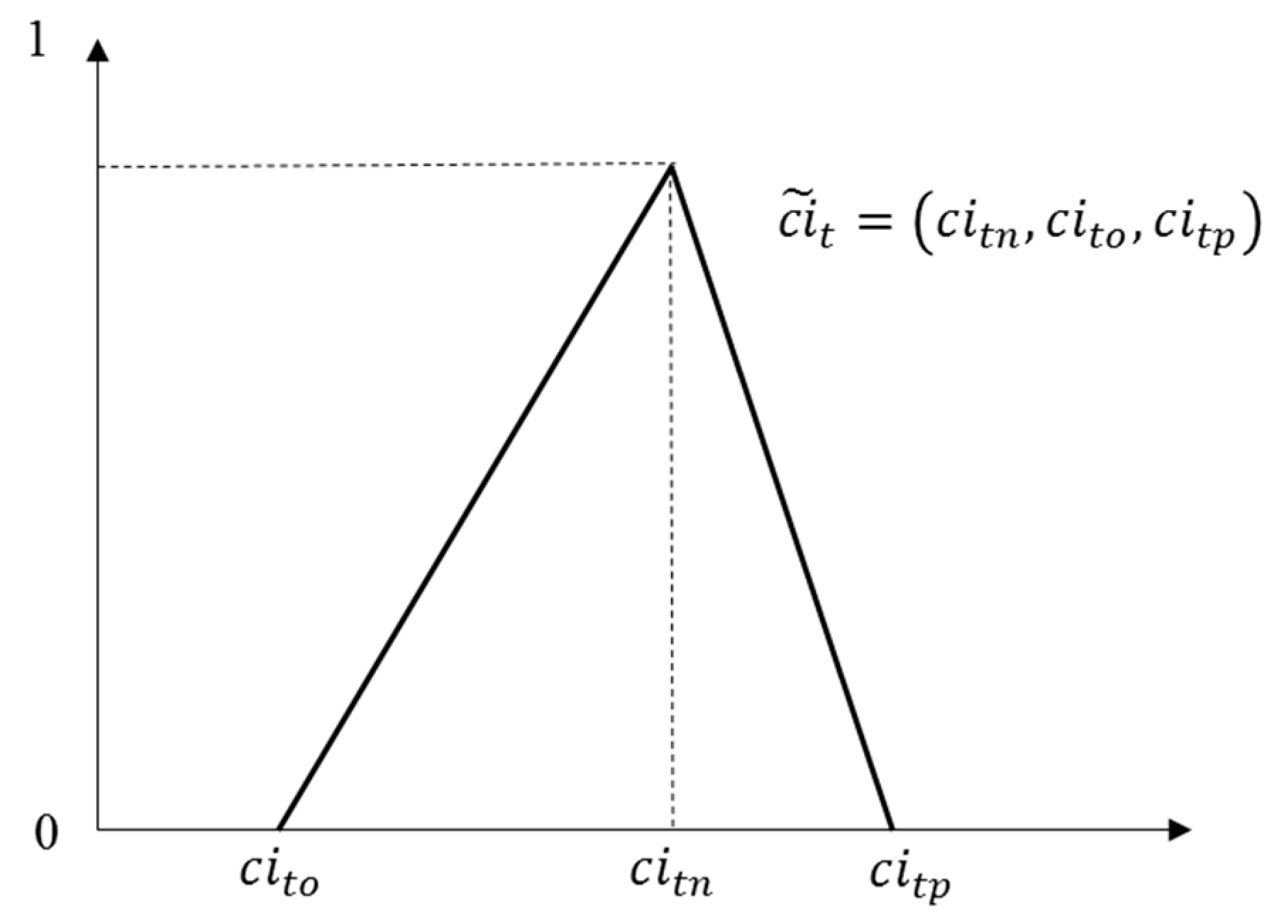
Objective Function (1) aims to minimize the total costs related to the procurements of water from the different sources, including storage costs and also fixed and variable procurement costs. Figure 1 shows a triangular possibility distribution, which represents the fuzziness of storage costs, ${\widetilde{ci}}_t=\left(c{i}_{tn},c{i}_{to},c{i}_{tp}\right)$, variable procurement cost, ${\widetilde{cpv}}_{imt}=\left(cp{v}_{imtn},cp{v}_{imto,}cp{v}_{imtp}\right),$ fixed procurement costs, ${\widetilde{cpf}}_{imt}=\left(cp{f}_{imtn},cp{f}_{imto,}cp{f}_{imtp}\right),$ and fixed procurement costs over the planning horizon, ${\widetilde{cf}}_{im}=\left(c{f}_{imn},c{f}_{imo,}c{f}_{imp}\right)$. This type of possibility distribution is represented by a triangular fuzzy number determined by the average or the most frequent value, the most optimistic, and the most pessimistic. For example, Figure 1 represents the possibility distribution for the fuzzy storage costs.

This is subject to:

$$S_t=S_{t-1}+{\displaystyle \sum }_i{\displaystyle \sum }_m{Q}_{imt}-d_t\hspace{1em}\hspace{1em}\hspace{1em}\forall t$$

(2)

Constraint (2) corresponds to the storage balance equation in the reservoirs.

$$S_t=S_{t-1}+{\displaystyle \sum }_i{\displaystyle \sum }_m{Q}_{imt}-d_t\hspace{1em}\hspace{1em}\hspace{1em}\forall t$$

(3)

$$S_t\le SMA{X}_t\hspace{1em}\hspace{1em}\hspace{1em}\forall t$$

(4)

Constraints (3) and (4) establish the safety stock and maximum storage capacity constraint, respectively.

$${\displaystyle \sum }_m{Q}_{imt}\le C{M}_{it}\hspace{1em}\hspace{1em}\hspace{1em}\forall i\forall t$$

(5)

Constraint (5) limits the required amounts from each source in each time period with respect to its maximum supply capacity.

$${\displaystyle \sum }_m{Y}_{imt}\le 1\hspace{1em}\hspace{1em}\hspace{1em}\forall i\forall t$$

(6)

Constraint (6) ensures that only one method is used for each source in each period.

$$Q_{imt}\le C{M}_{it}\cdot Y_{imt}\hspace{1em}\hspace{1em}\hspace{1em}\forall i\forall m\forall t$$

(7)

Constraint (7) generates the activation of decision variable Y_imt when decision variable Q_imt is higher than 0.

$${\displaystyle \sum }_m{\displaystyle \sum }_{t\in M_t^K}{Q}_{imt}\le CM{T}_{it}\hspace{1em}\hspace{1em}\hspace{1em}\forall i$$

(8)

$${\displaystyle \sum }_{t\in M_t^K}{Y}_{imt}\le C{H}_{im}\hspace{1em}\hspace{1em}\hspace{1em}\forall i\forall m$$

(9)

Constraints (8) and (9) correspond to the limitation of the monthly volume for each source and the time limitation for each source and method, respectively.

$$S_t,Q_{imt}\in ℝ$$

(10)

$$Y_{imt}, F_{im}\in \left\{0,1\right\}$$

(11)

The real and binary values for decision variables are determined by Constraints (10) and (11).

2.2. Solution Approaches

In this section, different approaches for considering fuzzy costs in mathematical programming models are applied to the previously presented model. The considered approaches are the first index of Yager, the third index of Yager, and Lai and Hwang’s approach.

A mathematical programming model with fuzzy costs may be formulated as follows:

$$\mathrm{Min}z= {\displaystyle \sum }_{j\in N}{\tilde{c}}_j{x}_j$$

(12)

$$\mathrm{s}.\mathrm{t}.{\displaystyle \sum }_{j\in N}{a}_{ij}{x}_j\le b_i\hspace{1em}\hspace{1em}\hspace{1em}i\in M$$

$$x_j\in ℝ\hspace{1em}\hspace{1em}j\in N$$

a_ij, b_i$\in$M, j$\in$N, and ${\tilde{c}}_j\in F(ℝ)$ where $F(ℝ)$ is the set of fuzzy numbers whose membership function ${\mu }_j$ represents the lack of precision of the values in objective function costs. The membership function is defined as follows:

$${\mu }_j:ℝ\to (0,1]\hspace{1em}j\in N$$

If triangular fuzzy numbers are considered in the form ${\tilde{c}}_j=\left(r_j,c_j,R_j\right)$, where r_j, c_j, and R_j correspond to the left (optimistic), center, and right (pessimistic) values, the membership function is given in the following way:

$$\forall u\in ℝ, j\in N,{\mu }_{c_j}\left(u\right)=\{\begin{array}{c}h\left(u\right)=\frac{\left(u-r_j\right)}{\left(c_j-r_j\right)},\hspace{1em}{r}_j\le u\le c_j\\ g\left(u\right)=\frac{\left(R_j-u\right)}{\left(r_j-c_j\right)},\hspace{1em}{c}_j\le u\le R_j\\ 0,\hspace{1em}\hspace{1em}\hspace{1em}otherwise\end{array}$$

(13)

According to Herrera and Verdegay [40,41], if the linear expression $\tilde{y}={\displaystyle \sum }_j{\tilde{c}}_j{x}_j$ is considered, in which ${\tilde{c}}_j$ are the fuzzy numbers with memebership functions similar to (13) and x_j ≥ 0, then the membership function of $\tilde{y}$ can be formulated as follows:

$$\mu \left(z\right)=\{\begin{array}{cc}\frac{\left(z-rx\right)}{\left(cx-rx\right)}& if rx\le z\le cx,\\ \frac{\left(Rx-z\right)}{\left(Rx-cx\right)}& if cx\le z\le Rx,\\ 0& otherwise\end{array}$$

(14)

where $r=\left(r_1,\dots ,r_n\right),c=\left(c_1,\dots ,c_n\right)$, and $R=\left(R_1,\dots ,R_n\right)$. The lateral margins (right and left, respectively) of the fuzzy number ${\tilde{c}}_j$ correspond to the expressions $d·x$ and $d\prime \cdot x$ if the vectors d and d′ are defined such that $d=R-c$ and $d^{\prime }=c-r$.

In order to obtain the optimal solution for (12), a ranking function f could be applied as Herrera and Verdegay [40,41] demonstrated. According to them, the first and third indices of Yager correspond to the following formulations.

2.2.1. First Index of Yager

The first function defuzzifies the uncertain costs by applying the concept of the center of gravity considering the following expression:

$$f_1\left({\tilde{u}}_j\right)=\frac{{{\displaystyle \int }}_0^{1}g\left(z\right){\mu }_{{\tilde{u}}_j}\left(z\right)dz}{{{\displaystyle \int }}_0^1{\mu }_{{\tilde{u}}_j}\left(z\right)dz}$$

(15)

where the measure of the importance of the value z is expressed by g(z). If linear weights and triangular fuzzy numbers are considered, the problem (12) corresponds to the following equivalent formulation [40,41]:

$$\mathrm{Min}z= \left(c+\left(d-d\prime \right)/3\right)x$$

(16)

$$\mathrm{s}.\mathrm{t}.\hspace{1em}\hspace{1em}\hspace{1em}Ax\le b$$

$$x_j\in ℝ\hspace{1em}\hspace{1em}\hspace{1em}j\in N$$

2.2.2. Third Index of Yager

The expression of the third index of Yager is as follows:

$$f_3\left({\tilde{u}}_j\right)={{\displaystyle \int }}_0^{1}M\left(U_j^{\alpha }\right)d\alpha$$

(17)

where $U_j^{\alpha }$ is the α-level set of ${\tilde{u}}_j$ and $M\left(U_j^{\alpha }\right)$ is the mean value of the elements of $U_j^{\alpha }$. Therefore, the optimal solution of (12) could be obtained by solving the following problem [40,41]:

$$\mathrm{Min}z= \left(c+\left(d-d\prime \right)/4\right)x$$

(18)

$$\mathrm{s}.\mathrm{t}.\hspace{1em}\hspace{1em}\hspace{1em}Ax\le b$$

$$x_j\in ℝ\hspace{1em}\hspace{1em}\hspace{1em}j\in N$$

2.2.3. Lai and Hwang’s Approach

Considering the problem defined by (12), each fuzzy cost is formulated as a triangular fuzzy number, which defines a fuzzy objective function with a triangular shape defined by the pessimistic, average or central, and optimistic values, according to the considered uncertain costs. In this sense, Lai and Hwang proposed to transform a mathematical programming model with fuzzy costs into a multiobjective mathematical programming model. This transformation was composed by three objective functions, which had the aim of minimizing the average costs (z₁), as well as the difference between pessimistic and average costs (z₃). Besides, simultaneously, the model maximized the difference between normal and optimistic costs (z₂). Thus, minimization of the original fuzzy objective can be obtained by pushing these three critical points in the direction of the left-hand side. Therefore, the following auxiliary problem is obtained taking into account the previous nomenclature:

$$\mathrm{Min}{z}_1= cx$$

(19)

$$\mathrm{Max}{z}_2= dx$$

$$\mathrm{Min}{z}_3= d\prime x$$

$$\mathrm{s}.\mathrm{t}.\hspace{1em}\hspace{1em}\hspace{1em}Ax\le b$$

$$x_j\in ℝ\hspace{1em}\hspace{1em}\hspace{1em}j\in N$$

In order to solve the obtained multiobjective mathematical programming model, several approaches can be applied, for example based on the use of fuzzy sets theory and goal programming. Readers are referred to the studies by Alavidoost et al. [42] and Torabi and Hassini [43].

2.3. Application of the Solution Approaches

2.3.1. First Index of Yager

According to the first index of Yager [40,41] the following equivalent model is obtained:

Objective function:

$$\begin{array}{cc}\hfill Min z=& {\displaystyle {\displaystyle \sum }_t}\frac{c{i}_{tn}+c{i}_{to}+c{i}_{tp}}{3}\cdot S_t\hfill \\ & +{\displaystyle {\displaystyle \sum }_i{\displaystyle \sum }_m{\displaystyle \sum }_t}\frac{cp{v}_{imtn}+cp{v}_{imto}+cp{v}_{imtp}}{3}\cdot Q_{imt}\hfill \\ & +{\displaystyle {\displaystyle \sum }_i{\displaystyle \sum }_m{\displaystyle \sum }_t}\frac{cp{f}_{imtn}+cp{f}_{imto}+cp{f}_{imtp}}{3}\cdot Y_{imt}\hfill \\ & +{\displaystyle {\displaystyle \sum }_i{\displaystyle \sum }_m}\frac{c{f}_{imn}+c{f}_{imo}+c{f}_{imp}}{3}\cdot F_{im}\hfill \end{array}$$

(20)

and Constraints (2) to (11).

2.3.2. Third Index of Yager

An auxiliary crisp model is obtained by applying the third index of Yager [44,45] for ranking fuzzy numbers as follows:

Objective function:

$$\begin{array}{cc}\hfill Min z=& {\displaystyle {\displaystyle \sum }_t}\frac{c{i}_{tn}+2c{i}_{to}+c{i}_{tp}}{4}\cdot S_t\hfill \\ & +{\displaystyle {\displaystyle \sum }_i{\displaystyle \sum }_m{\displaystyle \sum }_t}\frac{cp{v}_{imtn}+2cp{v}_{imto}+cp{v}_{imtp}}{4}\cdot Q_{imt}\hfill \\ & +{\displaystyle {\displaystyle \sum }_i{\displaystyle \sum }_m{\displaystyle \sum }_t}\frac{cp{f}_{imtn}+2cp{f}_{imto}+cp{f}_{imtp}}{4}\cdot Y_{imt}\hfill \\ & +{\displaystyle {\displaystyle \sum }_i{\displaystyle \sum }_m}\frac{c{f}_{imn}+2c{f}_{imo}+c{f}_{imp}}{4}\cdot F_{im}\hfill \end{array}$$

(21)

and Constraints (2) to (11).

2.3.3. Lai and Hwang’s Approach

The work in [46] introduced a solution method using uncertain costs, in which a fuzzy objective function is modelled with triangular possibility distributions into three different objective functions. According to [46], the original model for the management of water sources is converted into the following multiple objective model:

$$\begin{array}{cc}\hfill Min z_1=& {\displaystyle {\displaystyle \sum }_t}c{i}_{tn}\cdot S_t\hfill \\ & +{\displaystyle {\displaystyle \sum }_i{\displaystyle \sum }_m{\displaystyle \sum }_t}cp{v}_{imtn}\cdot Q_{imt}\hfill \\ & +{\displaystyle {\displaystyle \sum }_i{\displaystyle \sum }_m{\displaystyle \sum }_t}cp{f}_{imtn}\cdot Y_{imt}+{\displaystyle {\displaystyle \sum }_i{\displaystyle \sum }_m}c{f}_{imn}\cdot F_{im}\hfill \end{array}$$

(22)

$$\begin{array}{cc}\hfill Max z_2=& {\displaystyle {\displaystyle \sum }_t}\left(c{i}_{tn}-c{i}_{to}\right)\cdot S_t\hfill \\ & +{\displaystyle {\displaystyle \sum }_i{\displaystyle \sum }_m{\displaystyle \sum }_t}\left(cp{v}_{imtn}-cp{v}_{imto}\right)\cdot Q_{imt}\hfill \\ & +{\displaystyle {\displaystyle \sum }_i{\displaystyle \sum }_m{\displaystyle \sum }_t}\left(cp{f}_{imtn}-cp{f}_{imto}\right)\cdot Y_{imt}+{\displaystyle {\displaystyle \sum }_i{\displaystyle \sum }_m}\left(c{f}_{imn}-c{f}_{imo}\right)\cdot F_{im}\hfill \end{array}$$

(23)

$$\begin{array}{cc}\hfill Min z_3=& {\displaystyle {\displaystyle \sum }_t}\left(c{i}_{tp}-c{i}_{tn}\right)\cdot S_t\hfill \\ & +{\displaystyle {\displaystyle \sum }_i{\displaystyle \sum }_m{\displaystyle \sum }_t}\left(cp{v}_{imtp}-cp{v}_{imtn}\right)\cdot Q_{imt}\hfill \\ & +{\displaystyle {\displaystyle \sum }_i{\displaystyle \sum }_m{\displaystyle \sum }_t}\left(cp{f}_{imtp}-cp{f}_{imtn}\right)\cdot Y_{imt}{\displaystyle +{\displaystyle \sum }_i{\displaystyle \sum }_m}\left(c{f}_{imp}-c{f}_{imn}\right)\cdot F_{im}\hfill \end{array}$$

(24)

This model minimizes the most possible value of the uncertain costs (14), whereas it maximizes the possibility of obtaining the lowest costs (15) and minimizes the possibility of obtaining the highest costs (16). The rest of the model is composed of Constraints (2) to (11).

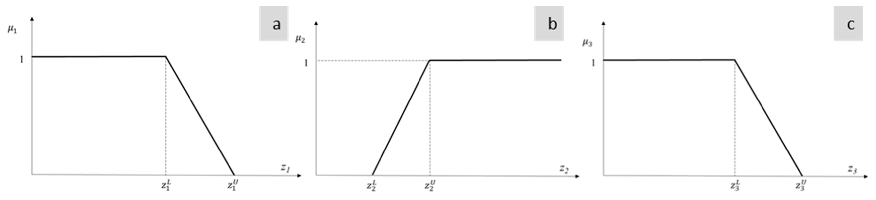
In order to solve the previous multiple objective model, applying the fuzzy goal programming approaches of Zimmermann [47], Werners [48], Selim and Ozkarahan [49], and Torabi and Hassini [43], the membership functions (μ₁, μ₂, μ₃) for each objective function (z₁, z₂, z₃) are formulated according to [50] as follows:

$${\mu }_1=\{\begin{array}{cc}1& z_1<z_1^l\\ \frac{z_1^u-z_1}{z_1^u-z_1^l}& z_1^l<z_1<z_1^u\\ 0& z_1>z_1^u\end{array}$$

(25)

$${\mu }_2=\{\begin{array}{cc}1& z_2>z_2^u\\ \frac{z_2-z_2^l}{z_2^u-z_2^l}& z_2^l<z_2<z_2^u\\ 0& z_2<z_2^l\end{array}$$

(26)

$${\mu }_3=\{\begin{array}{cc}1& z_3<z_3^l\\ \frac{z_3^u-z_3}{z_3^u-z_3^l}& z_3^l<z_3<z_3^u\\ 0& z_3>z_3^u\end{array}$$

(27)

where $z_1^l,z_2^l,z_3^l$ and $z_1^u,z_2^u,z_3^u$ are the lower and upper bounds of each objective function. These values can be determined by the decision-maker according to his/her experience and personal criteria or by minimizing and maximizing separately each objective function as suggested by several authors such as [45] or [49]. Figure 2 shows the boundaries of the membership curves denoted by Equations (25)–(27) related to the objective functions.

2.3.4. The Zimmerman Solution Method

The previous multiple objective linear programming model can be transformed into an equivalent model with a single objective, according to the approach of [46], maximizing an auxiliary variable ${\lambda }_0\in \left[0,1\right]$, which represents the minimum degree of fulfilment of all the objectives:

$$Max {\lambda }_0$$

(28)

subject to:

$$z_1\le z_1^u-{\lambda }_0\left(z_1^u-z_1^l\right)$$

(29)

$$z_2\ge z_2^l+{\lambda }_0\left(z_2^u-z_2^l\right)$$

(30)

$$z_3\le z_3^u-{\lambda }_0\left(z_3^u-z_3^l\right)$$

(31)

and Constraints (2) to (11).

2.3.5. The Werners Solution Method

According to [47], the multiple objective model can be transformed into an equivalent single objective models as follows:

$$Max \lambda \left(x\right)=\gamma {\lambda }_0+\left(1-\gamma \right)\frac{1}{3}\left({\lambda }_1+{\lambda }_2+{\lambda }_3\right)$$

(32)

subject to:

$$z_1\le z_1^u-\left({\lambda }_0+{\lambda }_1\right)\left(z_1^u-z_1^l\right)$$

(33)

$$z_2\ge z_2^l+\left({\lambda }_0+{\lambda }_2\right)\left(z_2^u-z_2^l\right)$$

(34)

$$z_3\le z_3^u-\left({\lambda }_0+{\lambda }_3\right)\left(z_3^u-z_3^l\right)$$

(35)

and Constraints (2) to (11).

Besides, λ₀ has an equivalent meaning to Zimmermann’s solution method. In contrast, γ corresponds to the compensation coefficient among the objectives.

2.3.6. Selim and Ozkarahan’s Solution Method

Based on the solution method proposed by [47,48], a new fuzzy goal programming approach was proposed based on a weighted sum to incorporate the relative importance degree of each objective function in order to represent the decision-maker’s preferences. The equivalent model obtained applying the Selim–Ozkarahan solution method is presented as follows:

$$Max \lambda \left(x\right)=\gamma {\lambda }_0+\left(1-\gamma \right)\left(w_1{\lambda }_1+w_2{\lambda }_2+w_3{\lambda }_3\right)$$

(36)

and Constraints (2) to (11) and (33) to (35).

2.3.7. Torabi and Hassini’s Solution Method

The fuzzy goal programming approach proposed by [49] considers a convex combination of the minimum satisfaction degree and the weighted sum of the membership function values for each objective function. In this sense, the obtained single objective equivalent crisp model applying the Torabi–Hassini approach is:

$$Max \lambda \left(x\right)=\gamma {\lambda }_0+\left(1-\gamma \right)\left(w_1{\mu }_1+w_2{\mu }_2+w_3{\mu }_3\right)$$

(37)

and Constraints (2) to (11) and (29) to (31).

Among the solution approaches considered, the first and third indices of Yager are characterized by their simplicity of application since they perform the defuzzification of uncertain values through average operations. The model considers the central, the more optimistic, and the more pessimistic values of the triangular fuzzy numbers. However, the approach proposed by Lai and Hwang is based on the resolution of a multi-objective mathematical programming model. If this proposal is compared with Yager’s indices, this presents a higher level of difficulty in order to obtain a solution by using additional proper solution methods, such as weighting objectives, the ξ-constraint, metaheuristics, or goal programming, among others. In this study, different fuzzy goal programming approaches have been considered. The obtained solution by applying Zimmerman’s [47] solution method might be neither unique nor efficient because it is focused on the optimization of the objective with a lower degree of satisfaction according to the decision-maker. Similar to Zimmerman’s approach, the Werners [48] solution method does not take into account the preferences of the decision-maker regarding their relative importance, although it introduces a compensation coefficient among them. In order to overcome the previous deficiencies, Selim and Ozkarahan [49] and Torabi and Hassini [43] presented solution methods in which the coefficient of compensation allowed accounting for the effect of the change in objective weights. According to [42], in these two approaches, a small change in the coefficient of compensation may yield a large amount of variability in the obtained solution (especially for lower values), and therefore, it is difficult to set this value in a precise way. Moreover, the formulations of Selim and Ozkarahan [49] and Torabi and Hassini [43] are more complex than those of Zimmerman or Werners and need more decision variables and computational time, but nevertheless, they can obtain better results.

3. Results and Discussion

3.1. Case Study

A real irrigation network was analyzed in order to show the innovation developed by this research. The water supply was used by [39] in order to analyze the necessary storage to supply the irrigation demand. The water system under study was located in Alicante province, supplying 260 hectares where there were vineyard crops. The water system was supplied from a small reservoir (its useful volume was 527,500 m³). The storage is defined as a function of water level using Equation (38):

S = 1259 WL² + 43,556 WL

(38)

where S is the storage in m³ and WL is the water level of the reservoir in m.

The consumption nodes (there were 110 irrigation consumption nodes) were located between 380 and 590 m above sea level. The pipelines that transport the water to the consumption nodes were manufactured from, iron and their range of diameters was from 80 to 550 mm.

The model was implemented with the MPL modelling language v5.0 [51], and the resolution was carried out with the optimization solver Gurobi v7.5.2 [52] in which a time limit of 180 s was set. Finally, it is worth mentioning that a Microsoft Access 2010 database managed the input and output data of the model.

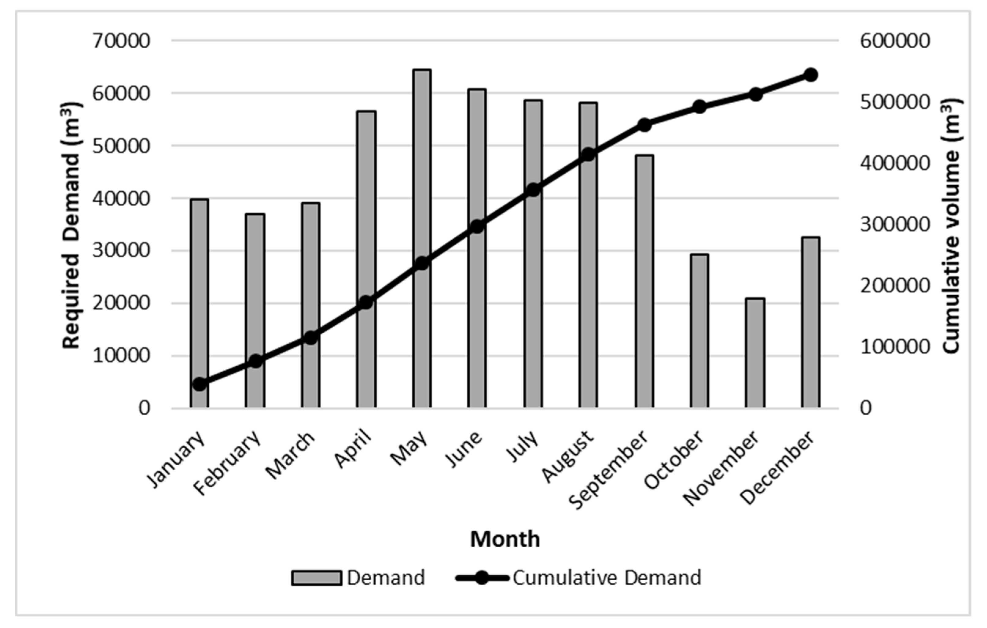
The data used in this model were the same as those used by [39] to make a comparison between both mathematical programming methods applied on the same water system. However, in this case, the total costs were determined considering the cumulative storage cost to make possible the comparison among the different proposed methods. Figure 3 shows the water demand of the case study for each month, as well as the annual cumulative required water. This water demand was satisfied from different water sources. Source 1 came from water transfer of another basin, and its price was fixed over time. The water of Source 2 was obtained from wastewater treatment, and its price was also fixed over time. Finally, the water from Source 3 came from desalination. The prices of Sources 4 and 5 were variable since they came from wells, and therefore; their prices depended on the energy price.

Table 2. Water prices as a function of the different sources according to [39].

Source	Method	Price
		(€/m3)
Source 1	Fixed	0.25
Source 2	Fixed	0.35
Source 3	Fixed	0.60
Source 4	Variable	−
	P1	0.56
	P2	0.50
	P3	0.35
	P4	0.30
	P5	0.20
	P6	0.12
Source 5	Variable	−
	P1	0.70
	P2	0.65
	P3	0.49
	P4	0.42
	P5	0.35
	P6	0.25

shows water prices for each of the five water sources. When the price was variable (Sources 4 and 5), the water price was also variable, and therefore, Table 2 shows the price for each period depending on the type of agreement (

Table 3. Period differentiation as a function of hour and month to define the energy consumption.

Hour	Month
	January	February	March	April	May	1–15 June	16–30 June	July	August	September	October	November	December
0	P6	P6	P6	P6	P6	P6	P6	P6	P6	P6	P6	P6	P6
1	P6	P6	P6	P6	P6	P6	P6	P6	P6	P6	P6	P6	P6
2	P6	P6	P6	P6	P6	P6	P6	P6	P6	P6	P6	P6	P6
3	P6	P6	P6	P6	P6	P6	P6	P6	P6	P6	P6	P6	P6
4	P6	P6	P6	P6	P6	P6	P6	P6	P6	P6	P6	P6	P6
5	P6	P6	P6	P6	P6	P6	P6	P6	P6	P6	P6	P6	P6
6	P6	P6	P6	P6	P6	P6	P6	P6	P6	P6	P6	P6	P6
7	P6	P6	P6	P6	P6	P6	P6	P6	P6	P6	P6	P6	P6
8	P2	P2	P4	P5	P5	P4	P2	P2	P6	P4	P5	P4	P2
9	P2	P2	P4	P5	P5	P3	P2	P2	P6	P4	P5	P4	P2
10	P1	P1	P4	P5	P5	P3	P2	P2	P6	P4	P5	P4	P1
11	P1	P1	P4	P5	P5	P3	P1	P1	P6	P4	P5	P4	P1
12	P1	P1	P4	P5	P5	P3	P1	P1	P6	P4	P5	P4	P1
13	P2	P2	P4	P5	P5	P3	P1	P1	P6	P4	P5	P4	P2
14	P2	P2	P4	P5	P5	P3	P1	P1	P6	P4	P5	P4	P2
15	P2	P2	P4	P5	P5	P4	P1	P1	P6	P4	P5	P4	P2
16	P2	P2	P3	P5	P5	P4	P1	P1	P6	P3	P5	P3	P2
17	P2	P2	P3	P5	P5	P4	P1	P1	P6	P3	P5	P3	P2
18	P1	P1	P3	P5	P5	P4	P1	P1	P6	P3	P5	P3	P1
19	P1	P1	P3	P5	P5	P4	P2	P2	P6	P3	P5	P3	P1
20	P1	P1	P3	P5	P5	P4	P2	P2	P6	P3	P5	P3	P1
21	P2	P2	P3	P5	P5	P4	P2	P2	P6	P3	P5	P3	P2
22	P2	P2	P4	P5	P5	P4	P2	P2	P6	P4	P5	P4	P2
23	P2	P2	P4	P5	P5	P4	P2	P2	P6	P4	P5	P4	P2

). The possibility distributions associated with uncertain costs were modelled using triangular fuzzy numbers, which were constructed setting a maximum deviation of 15% for the most optimistic costs and 25% for the most pessimistic costs with respect to the most frequent ones.

With regard to the variable costs, they were related to the energy price. In Spain, there are different agreements that regulate this aspect. One of the agreements considers six periods from P1 to P6. Each period depends on the hour and date according to Table 3.

Moreover, the maximum supply capacity of each source is shown in

Table 4. Maximum supply capacity of each source.

Source	Hourly Capacity (m3) CMit	Monthly Capacity (m3) CMTit
1	120	40,000
2	306	500,000
3	324	75,000
4	360	75,000
5	450	125,000

. The data are expressed in hourly and monthly capacity per source. Additionally, Sources 4 and 5 had a limited number of hours for supplying water depending on the month and the selected method (

Table 5. Limitation of hours for supplying water for Sources 4 and 5.

		Hours of Water Service Per Month
Source	Method	1	2	3	4	5	6	7	8	9	10	11	12
4	2	132	120	0	0	0	0	286	0	0	0	0	126
4	3	220	200	0	0	0	0	66	0	0	0	0	210
4	4	0	0	126	0	0	126	0	0	120	0	126	0
4	5	0	0	210	0	0	210	0	0	200	0	210	0
4	6	0	0	0	336	336	0	0	0	0	352	0	0
4	7	392	352	408	384	408	384	392	744	400	392	384	456
5	2	132	120	0	0	0	0	286	0	0	0	0	126
5	3	220	200	0	0	0	0	66	0	0	0	0	210
5	4	0	0	126	0	0	126	0	0	120	0	126	0
5	5	0	0	210	0	0	210	0	0	200	0	210	0
5	6	0	0	0	336	336	0	0	0	0	352	0	0
5	7	392	352	408	384	408	384	392	744	400	392	384	456

).

3.2. Results

Table 6. Optimization results of the model statistics (€).

	First Index of Yager	Third Index of Yager	Lai and Hwang Approach
			Zimmerman’s Approach	Werners’ Approach	Selim and Ozkarahan’s Approach	Torabi and Hassini’s Approach
Total costs (z)	285,753	284,076	-	-	-	-
Most possible total costs (z1)	-	-	278,579	278,567	278,450	278,531
Most optimistic total costs (z2)	-	-	236,792	236,782	236,683	236,752
Most pessimistic total costs (z3)	-	-	348,224	348,209	348,063	348,164
Computational Time	-	30%	294%	350%	322%	229%

Solution parameter settings: γ = 0.4; w₁ = 0.6; w₂ = 0.2; w₃ = 0.2.

summarizes the solutions yielded by the proposed models. From Table 6, it can be determined that the two models, based on the first and third indices of Yager, provided the worst results in terms of total costs compared to Lai and Hwang’s approach. In this sense, Lai and Hwang’s approach (1992) generated four different fuzzy solutions, depending on the solution method applied. Among them, Selim and Ozkarahan’s approach obtained the best solution in terms of most possible (z₁), most optimistic (z₂), and most pessimistic (z₃) total costs. Therefore, the decision-maker could develop a water management plan with a triangular possibility distribution for total storage and procurements costs (z₁, z₂, z₃) = (278,450, 236,683, 348,063).

Table 6 also shows the computational time used by each model as the percentage of the one used by the first index of Yager to highlight the order of magnitude of additional computation. As can be seen, although there were differences among the different methods, these were not significant as the solutions tended to be rather fast.

If Table 6 is analyzed in order to compare the results for each model used, considering the first index of Yager (FY) as the basis of the comparison, the total cost of the third index of Yager was 1% lower. The most possible total costs (z₁) when Lai and Hwang’s approach was used was 97.4% comparing it to FY. The different approaches varied between 278,450 (Selim and Ozkarahan’s approach) and 278,579 € (Zimmerman’s approach). However, the variation between the maximum and minimum costs was 0.05%. Therefore, the use of the different approaches was indifferent with respect to obtaining the optimal solution. When the most optimistic and pessimistic costs were analyzed (Table 6), a reduction of 17.8% was obtained, while the pessimistic costs showed an increase of 21.86 %. The annual volume used of each source as a function of the considered solution approach is shown in

Table 7. Comparison of annual volume and percentage of use.

Source	Method	Annual Volume (m3/Year)	% Use with Respect to Annual Capacity of Each Water Source Used
First Index of Yager
4	7	347,743	38.64%
Third Index of Yager
4	7	347,743	38.64%
Zimmerman’s approach
1	1	36	0.01%
4	7	347,743	38.64%
Werners’ approach
1	1	2565	0.53%
2	1	343,111	5.72%
3	1	1797	0.20%
Selim and Ozkarahan’s approach
1	1	4489	0.94%
2	1	951	0.02%
4	7	346,457	38%
Torabi and Hassini’s approach
1	1	1970	0.41%
2	1	5454	0.09%
4	7	340,049	37.78%

. Besides, Table 7 shows the percentage used of each considered water source for each solution approach.

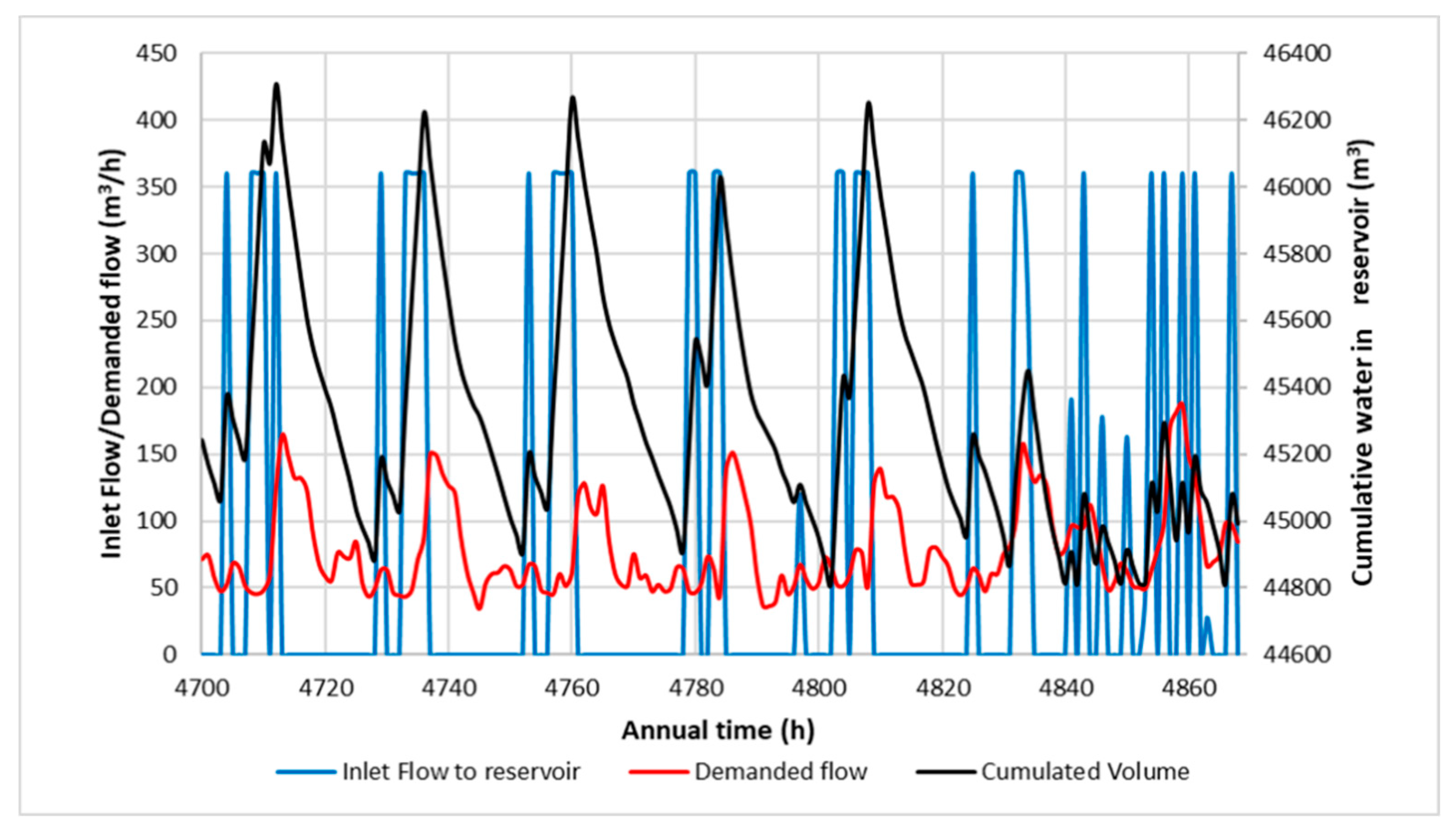
Figure 4 shows an example of the water system management by using linear programming with Selim and Ozkarahan’s approach. When all results over time were examined, Source 1 had a frequency of 19.7%. The frequency related to Source 2 was 1.13%, and the rest of the time, the water was obtained from Source 4 considering the energy period P6. Therefore, Source 4 was the main one used to minimize the exploitation cost of the water system. This trend was similar for the different statistics models developed in this research, where Source 4 was the main source to supply the water demand, considering P6.

Regarding the operation of the irrigation system, Figure 4 shows the third week of June, for which the cumulative volume in the reservoir (i.e., storage) oscillated between 46,308 and 44,815 m³. This trend was stable over the planning horizon once the water system reached continuous time. Therefore, the planning demonstrated that it was not necessary to reach the maximum water level in the reservoir in the winter season since the water sources were enough to meet the annual water demand, minimizing the exploitation costs. Accordingly, the proposed model showed a significant improvement in comparison with the results given by the water manager, enhancing the current management [26]. In this sense, the proposed model allowed distributing the energy, storage, and management costs over the planning horizon simultaneously with incomes provided from selling water to farmers. Otherwise, the current planning method used by water manager concentrates most of the amounts of required water in winter months, and consequently, it is necessary to have large flows of cash available or, in some cases, to apply for loans from credit institutions.

Table 8. Model statistics.

	First Index of Yager	Third Index of Yager	Lai and Hwang Approach
			Zimmerman’s Approach	Werners’ Approach	Selim and Ozkarahan’s Approach	Torabi and Hassini’s Approach
Constraints	455,654	455,654	455,661	455,661	455,661	455,661
Variables	96,372	96,372	96,376	96,379	96,379	96,376
Integers	43,812	43,812	43,812	43,812	43,812	43,812
Nonzeros	2,417,737	2,417,737	2,803,234	2,803,237	2,803,237	2,803,234
Density	0.006%	0.006%	0.006%	0.006%	0.006%	0.006%
Iterations	19,875	19,858	68,620	36,858	35,569	34,532
Solution time (s)	22	28	85	97	91	76

presents the computational efficiency of the evaluated models. The results, from a computational viewpoint, were obtained by setting an upper bound of CPU time limited at 180 s and a stopping criterion for the gap of 0.5% so that the computational process stopped if either criterion was met. Moreover, data related to the number of constraints, decision variables, integer elements, and the nonzero and density of the coefficient matrix (defined as the percentage of nonzero coefficients in the total number of coefficients) are shown. The number of decision variables should be obtained by multiplying the size dimensions of each variable. However, in order to obtain a better computational performance, some filters related to impossible combinations of decision variables related to the case study were applied. As the evaluated models had a similar structure and the same input data, number of variables, integers, and constraints, the comparison presented very small or null variations. For example, the number of integer elements was the same for all the considered approaches, while the number of constraints and variables was slightly higher for Lai and Hwang’s approach, and particularly so for Werners’ and Selim and Ozkarahan’s approaches. On the other hand, the number of nonzero elements was considerable higher for all the solution methods associated with Lai and Hwang’s approach in comparison with Yager’s indices.

Table 8 also shows how Lai and Hwang’s approach required a considerably higher amount of CPU time compared to Yager’s approaches. Moreover, the different approaches to solve Lai and Hwang’s model also needed a higher number of iterations to obtain an optimal mixed integer linear programming solution, especially Zimmerman’s solution method. Additionally, although Lai and Hwang’s approach had a larger number of constraints and integer variables, this does not imply additional information storage requirements, but an increased modelling complexity. Finally, Werners’ model and mainly Selim-Ozkarahan’s and Torabi-Hassini’s approaches required more parameter settings for the decision-maker.

4. Conclusions

Different solution approaches were applied and evaluated in terms of model complexity and computational efficiency, and the solution accomplished was presented. Lai and Hwang’s approach, which was solved by Werners’ method, implied more modelling complexity and CPU time, but provided more flexibility for decision-makers to achieve a fuzzy solution according to their preferences.

When the comparison was applied to a real water network, Lai and Hwang’s approach reached the best solution in which the reduction of total costs was near 20% compared to the first index of Yager. The decrease of operational costs was very significant since this reduction was directly related to the reduction of energy consumption (e.g., pumped water or wastewater treatment, which established the water price). Therefore, a sustainability increase was reached when the decrease of costs was achieved.

Finally, the manuscript enables developing further lines of research. These lines can be focused on: (1) testing the models with real-world problems in a rolling horizon; (2) comparing the models with other solution approaches; (3) using other membership functions patterns; (4) including carbon footprint and the selection of sources of energy; (5) incorporating financial issues in order to optimize the generated cash flows and therefore improve the cost effectiveness.

References

- Biswas, A.K. Integrated water resources management: A reassessment: A water forum contribution. Water Int. 2004, 29, 248–256. [Google Scholar] [CrossRef]
- Pahl-Wostl, C. Transitions towards adaptive management of water facing climate and global change. Water Resour. Manag. 2007, 21, 49–62. [Google Scholar] [CrossRef]
- Wu, K.K.; Zhang, L.P. Progress in the development of environmental risk assessment as a tool for decision-making process. J. Serv. Sci. Manag. 2014, 7, 131–144. [Google Scholar] [CrossRef]
- Hernández-Bedolla, J.; Solera, A.; Paredes-Arquiola, J.; Pedro-Monzonís, M.; Andreu, J.; Sánchez-Quispe, S. The assessment of sustainability indexes and climate change impacts on integrated water resource management. Water 2017, 3, 213. [Google Scholar] [CrossRef]
- Hunink, J.; Simons, G.; Suárez-Almiñana, S.; Solera, A.; Andreu, J.; Giuliani, M.; Schasfoort, F. A simplified water accounting procedure to assess climate change impact on water resources for agriculture across different European river basins. Water 2019, 11, 1976. [Google Scholar] [CrossRef]
- Pérez-Sánchez, M.; Sánchez-Romero, F.J.; Ramos, H.R.; López Jiménez, P.A. Modeling irrigation networks for the quantification of potential energy recovering: A case study. Water 2016, 6, 234. [Google Scholar] [CrossRef]
- Corominas, J. Agua y energía en el riego, en la época de la sostenibilidad. Ing. Agua 2010, 17, 219–233. [Google Scholar] [CrossRef]
- Romero, L.; Pérez-Sánchez, M.; López Jiménez, P.A. Improvement of sustainability indicators when traditional water management changes: A case study in Alicante (Spain). AIMS Environ. Sci. 2017, 3, 502–522. [Google Scholar] [CrossRef]
- Davies, E.G.; Simonovic, S.P. Global water resources modeling with an integrated model of the social-economic-environmental system. Adv. Water Resour. 2011, 34, 684–700. [Google Scholar] [CrossRef]
- Alcamo, J.; Döll, P.; Henrichs, T.; Kaspar, F.; Lehner, B.; Rösch, T.; Siebert, S. Development and testing of the WaterGAP 2 global model of water use and availability. Hydrol. Sci. J. 2003, 48, 317–337. [Google Scholar] [CrossRef]
- Sanchis, R.; Poler, R. Enterprise resilience assessment—A quantitative approach. Sustainability 2019, 11, 4327. [Google Scholar] [CrossRef]
- Rahaman, M.M.; Varis, O. Integrated water resources management: Evolution, prospects and future challenges. Sustain. Sci. Pract. Policy. 2005, 1, 15–21. [Google Scholar] [CrossRef]
- Markantonis, V.; Arnaud, R.; Karabulut, A.; El Hajj, R.; Altinbilek, D.; Awad, I.; Brugemann, A.; Vangelis, C.; Mysiak, J.; Lamaddalena, N.; et al. Can the implementation of the water-energy-food nexus support economic growth in the Mediterranean region? The current status and the way forward. Front. Env. Sci. 2019, 7, 84. [Google Scholar] [CrossRef]
- Copeland, C. Energy Water Nexus: The Water Sector’s Energy Use; Congressional Research Service: Washington, DC, USA, 2014. [Google Scholar]
- Food and Agriculture Organization (FAO). Available online: www.fao.org (accessed on 2 September 2019).
- Tsur, Y. Water pricing. Agric. Appl. Econ. Assoc. 2019. [Google Scholar] [CrossRef]
- Schleich, J.; Hillenbrand, T. Water Demand Responds Asymmetrically to Rising and Falling Prices; No. S03/2019; Working Paper Sustainability and Innovation; Fraunhofer Institute for Systems and Innovation Research: Karlsruhe, Germany, 2019. [Google Scholar]
- Directive 2000/60/EC of the European Parliament and of the Council. Available online: https://eur-lex.europa.eu/eli/dir/2000/60/oj (accessed on 3 June 2019).
- Namany, S.; Al-Ansari, T.; Govindan, R. Sustainable energy, water and food nexus systems: A focused review of decision-making tools for efficient resource management and governance. J. Clean. Prod. 2019, 225, 610–626. [Google Scholar] [CrossRef]
- Archibald, T.W.; Marshall, S.E. Review of mathematical programming applications in water resource management under uncertainty. Env. Model. Assess. 2018, 23, 753–777. [Google Scholar] [CrossRef]
- Chen, S.; Shao, D.; Gu, W.; Xu, B.; Li, H.; Fang, L. An interval multistage water allocation model for crop different growth stages under inputs uncertainty. Agric. Water Manag. 2017, 186, 86–97. [Google Scholar] [CrossRef]
- Xie, Y.L.; Xia, D.H.; Huang, G.H.; Li, W.; Xu, Y. A multistage stochastic robust optimization model with fuzzy probability distribution for water supply management under uncertainty. Stoch. Env. Res. Risk. 2017, 31, 125–143. [Google Scholar] [CrossRef]
- Heumesser, C.; Fuss, S.; Szolgayová, J.; Strauss, F.; Schmid, E. Investment in irrigation systems under precipitation uncertainty. Water Resour. Manag. 2012, 26, 3113–3137. [Google Scholar] [CrossRef]
- Pereira-Cardenal, S.J.; Mo, B.; Riegels, N.D.; Arnbjerg-Nielsen, K.; Bauer-Gottwein, P. Optimization of multipurpose reservoir systems using power market models. J. Water Res. Plan. Man. 2015, 141, 8. [Google Scholar] [CrossRef]
- Kumari, S.; Mujumdar, P.P. Fuzzy set-based system performance evaluation of an irrigation reservoir system. J. Irrig. Drain. Eng. 2017, 143, 5. [Google Scholar] [CrossRef]
- Jairaj, P.G.; Vedula, S. Multireservoir system optimization using fuzzy mathematical programming. Water Resour. Manag. 2000, 14, 457–472. [Google Scholar] [CrossRef]
- Li, M.; Guo, P.; Singh, V.P.; Zhao, J. Irrigation water allocation using an inexact two-stage quadratic programming with fuzzy input under climate change. J. Am. Water Resour. 2016, 52, 667–684. [Google Scholar] [CrossRef]
- Bozorg-Haddad, O.; Malmir, M.; Mohammad-Azari, S.; Loáiciga, H.A. Estimation of farmers’ willingness to pay for water in the agricultural sector. Agric. Water Manag. 2016, 177, 284–290. [Google Scholar] [CrossRef]
- An-Vo, D.A.; Mushtaq, S.; Reardon-Smith, K. Estimating the value of conjunctive water use at a system-level using nonlinear programming model. J. Econ. Soc. Policy 2014, 17, 1–20. [Google Scholar]
- Raju, K.S.; Duckstein, L. Multiobjective fuzzy linear programming for sustainable irrigation planning: An Indian case study. Soft Comput. 2003, 7, 412–418. [Google Scholar] [CrossRef]
- Regulwar, D.G.; Gurav, J.B. Sustainable irrigation planning with imprecise parameters under fuzzy environment. Water Resour. Manag. 2012, 26, 3871–3892. [Google Scholar] [CrossRef]
- Mula, J.; Poler, R.; García, J.P. Capacity and material requirement planning modelling by comparing deterministic and fuzzy models. Int. J. Prod. Res. 2008, 6, 5589–5606. [Google Scholar] [CrossRef]
- Díaz-Madroñero, M.; Mula, J.; Jiménez, M.; Peidro, D. A rolling horizon approach for material requirement planning under fuzzy lead times. Int. J. Prod. Res. 2017, 55, 2197–2211. [Google Scholar] [CrossRef]
- Mula, J.; Díaz-Madroñero, M. Solution approaches for material requirement planning* with fuzzy costs. In Industrial Engineering: Innovative Networks; Sethi, S., Bogataj, M., Ros-McDonnell, L., Eds.; Springer: Berlin, Germany, 2012; pp. 349–357. [Google Scholar]
- Mula, J.; Poler, R.; Garcia, J.P. MRP with flexible constraints: A fuzzy mathematical programming approach. Fuzzy Sets Syst. 2006, 157, 74–97. [Google Scholar] [CrossRef]
- Mula, J.; Poler, R.; Garcia-Sabater, J.P. Material requirement planning with fuzzy constraints and fuzzy coefficients. Fuzzy Sets Syst. 2007, 158, 783–793. [Google Scholar] [CrossRef]
- Díaz-Madroñero, M.; Mula, J.; Jiménez, M. Fuzzy goal programming for material requirements planning under uncertainty and integrity conditions. Int. J. Prod. Res. 2014, 52, 6971–6988. [Google Scholar] [CrossRef]
- Peidro, D.; Díaz-Madroñero, M.; Mula, J. An Interactive fuzzy multi-objective approach for operational transport planning in an automobile supply chain. WSEAS Trans. Inf. Sci. Appl. 2010, 7, 283–294. [Google Scholar]
- Pérez-Sánchez, M.; Díaz-Madroñero Boluda, F.M.; López Jiménez, P.A.; Mula, J. Mathematical programming model for procurement selection in water irrigation systems. A case study. J. Eng. Sci. Technol. Rev. 2017, 6, 146–153. [Google Scholar] [CrossRef]
- Herrera, F.; Verdegay, J.L. Three models of fuzzy integer linear programming. Eur. J. Oper. Res. 1995, 83, 581–593. [Google Scholar] [CrossRef]
- Herrera, F.; Verdegay, J.L. Fuzzy boolean programming problems with fuzzy costs: A general study. Fuzzy Set Syst. 1996, 81, 57–76. [Google Scholar] [CrossRef]
- Alavidoost, M.H.; Babazadeh, H.; Sayyari, S.T. An interactive fuzzy programming approach for bi-objective straight and U-shaped assembly line balancing problem. Appl. Soft Comput. 2016, 40, 221–235. [Google Scholar] [CrossRef]
- Yager, R.R. Ranking fuzzy subsets over the unit interval. In Proceedings of the IEEE Conference on. Decision and Control, San Diego, CA, USA, 10–12 January 1979; pp. 1435–1437. [Google Scholar]
- Torabi, S.A.; Hassini, E. An interactive possibilistic programming approach for multiple objective supply chain master planning. Fuzzy Sets Syst. 2008, 159, 193–214. [Google Scholar] [CrossRef]
- Yager, R.R. A procedure for ordering fuzzy subsets of the unit interval. Inf. Sci. 1981, 24, 143–161. [Google Scholar] [CrossRef]
- Lai, Y.J.; Hwang, C.L. A new approach to some possibilistic linear programming problems. Fuzzy Sets Syst. 1992, 49, 121–133. [Google Scholar] [CrossRef]
- Zimmermann, H.J. Fuzzy programming and linear programming with several objective functions. Fuzzy Sets Syst. 1978, 1, 45–55. [Google Scholar] [CrossRef]
- Werners, B. Aggregation models in mathematical programming. In Mathematical Models for Decision Support; Mitra, G., Greenberg, H.J., Lootsma, F.A., Rijckaert, M.J., Zimmermann, H.-J., Eds.; Springer: Berling/Heidelberg, Germany, 1988; pp. 295–305. [Google Scholar]
- Selim, H.; Ozkarahan, I. A supply chain distribution network design model: An interactive fuzzy goal programming-based solution approach. Int. J. Adv. Manuf. Technol. 2008, 36, 401–418. [Google Scholar] [CrossRef]
- Bellman, R.; Zadeh, L. Decision making in a fuzzy environment. Manag. Sci. 1970, 17, 141–164. [Google Scholar] [CrossRef]
- Maximal Software Incorporation. MPL Modeling System, Release 5.0; Maximal Software Incorporation: Arlington, VA, USA, 2016. [Google Scholar]
- Gurobi Optimization, Incorporation. Gurobi Optimizer Reference Manual, Release 7.5.2; Gurobi Optimization: Beaverton, OR, USA, 2017. [Google Scholar]
Figure 1.
Triangular possibility distribution.
Figure 2.
Membership curves for the objective functions for (a), (b), and (c) (adapted from [46,47,48,49]).
Figure 3.
Data of the water demand according to [30].
Figure 4.
Example of demanded sources in the third week of June by applying Selim and Ozkarahan’s approach.