Identifying Efficient Operating Rules for Hydropower Reservoirs Using System Dynamics Approach—A Case Study of Three Gorges Reservoir, China

 , , and
Abstract
:1. Introduction
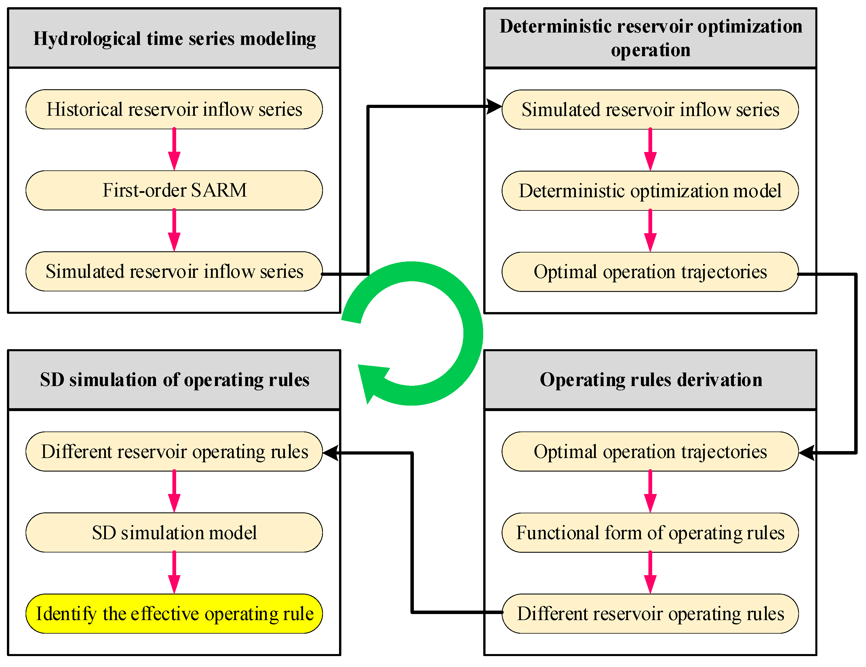
2. Methods
2.1. Hydrological Time Series Modelling
2.1.1. Pre-Processing of Historical Inflow Series
2.1.2. First-Order Seasonal Autoregressive Model
2.2. Deterministic Reservoir Optimization Operation Model
2.2.1. Objective Function
2.2.2. Constraints
2.2.3. Solution
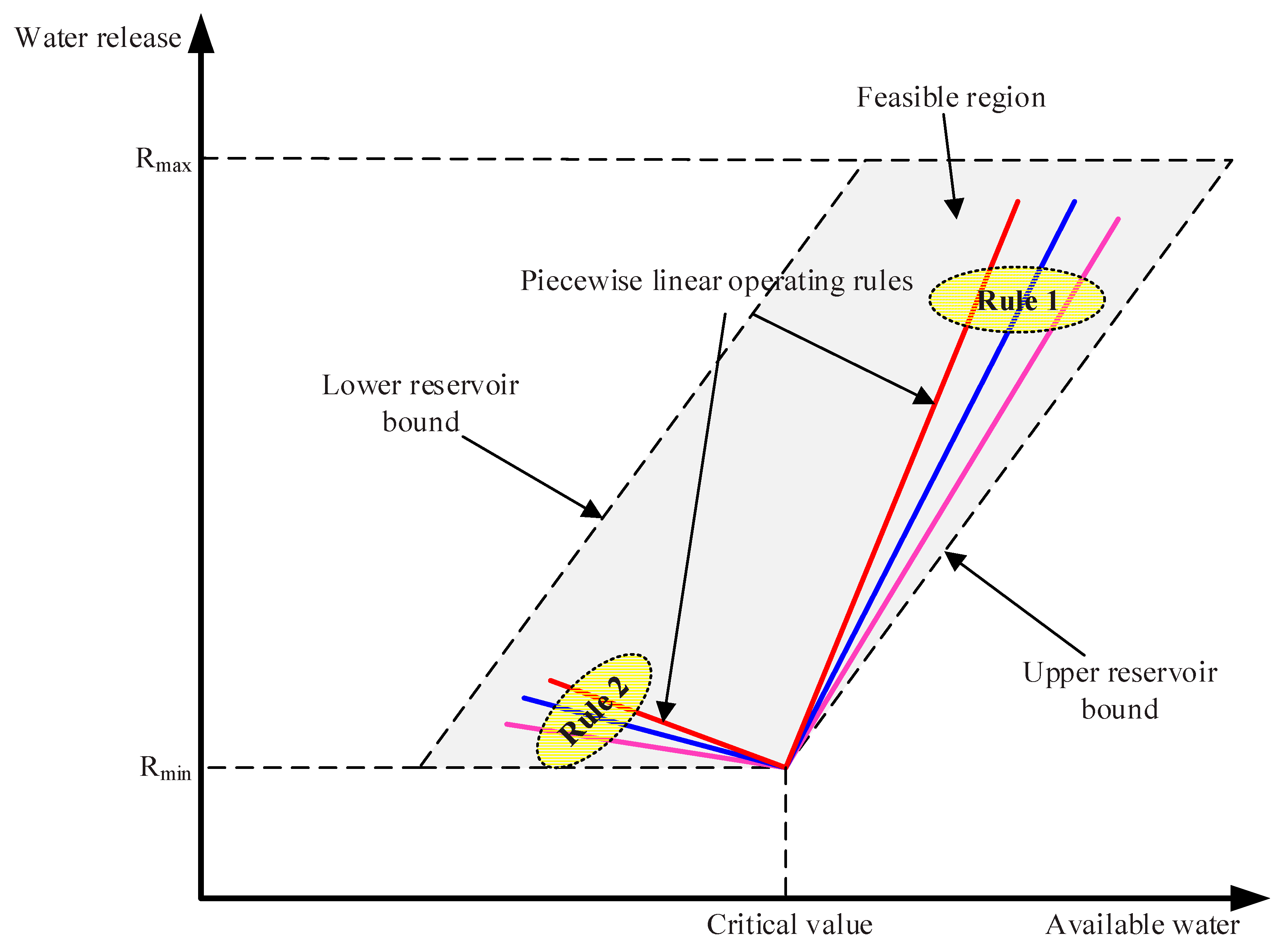
2.3. Reservoir Operating Rules Derivation
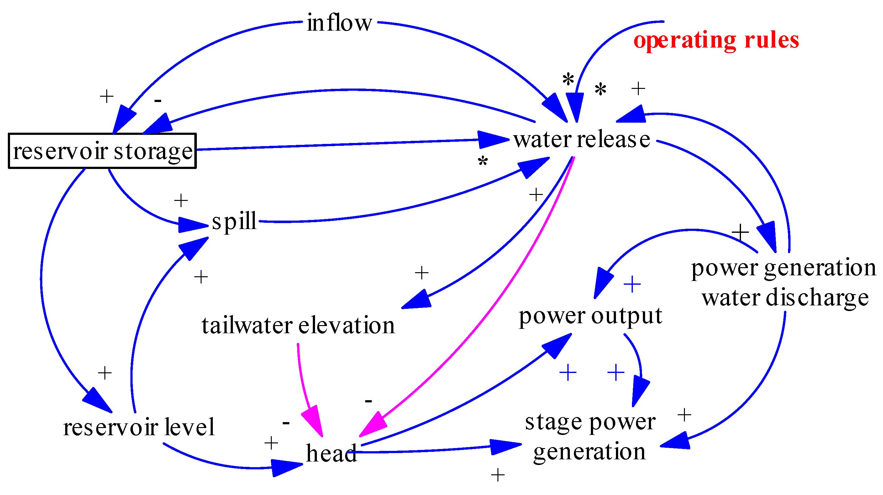
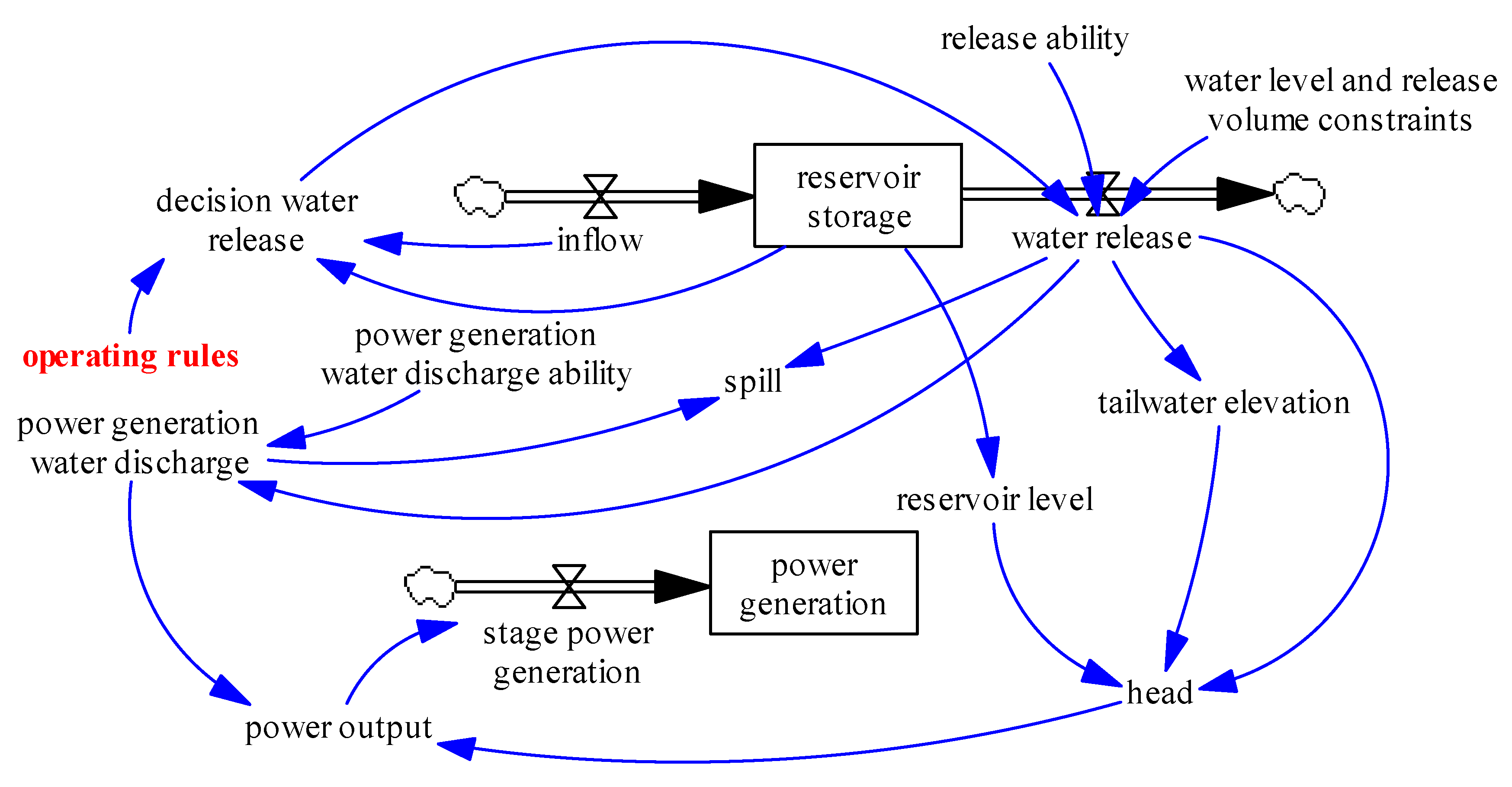
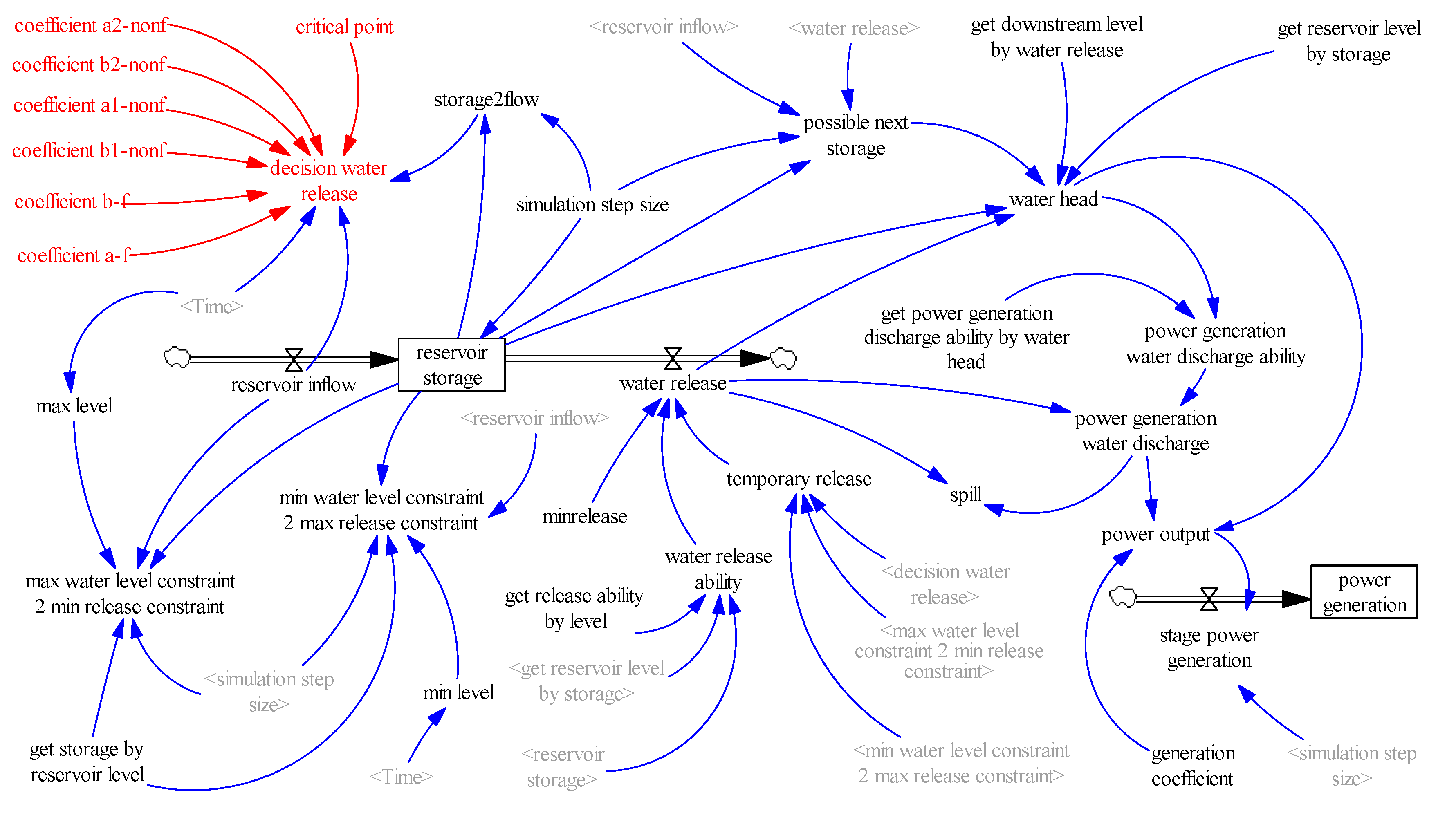
2.4. System Dynamics Simulation Model of Hydropower Reservoir Operation
3. Case Study
3.1. The Three Gorges Reservoir
3.2. Results
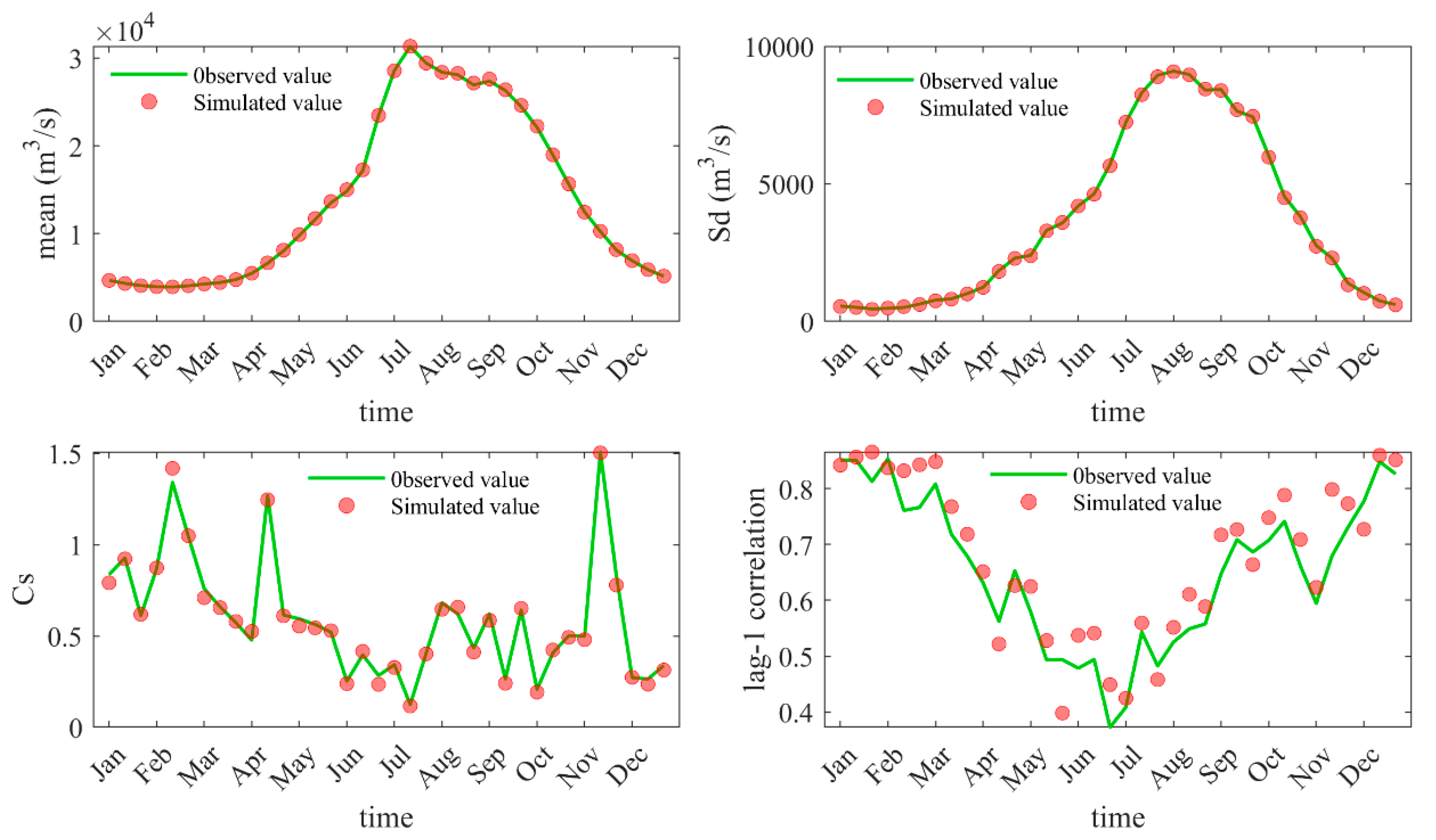
3.2.1. Simulated Reservoir Inflow Series Based on the First-Order SARM
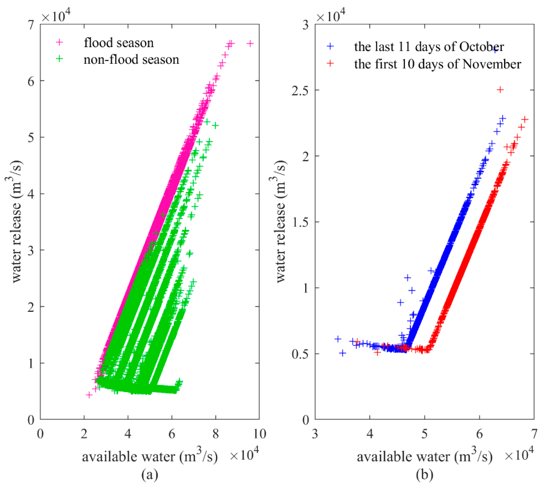
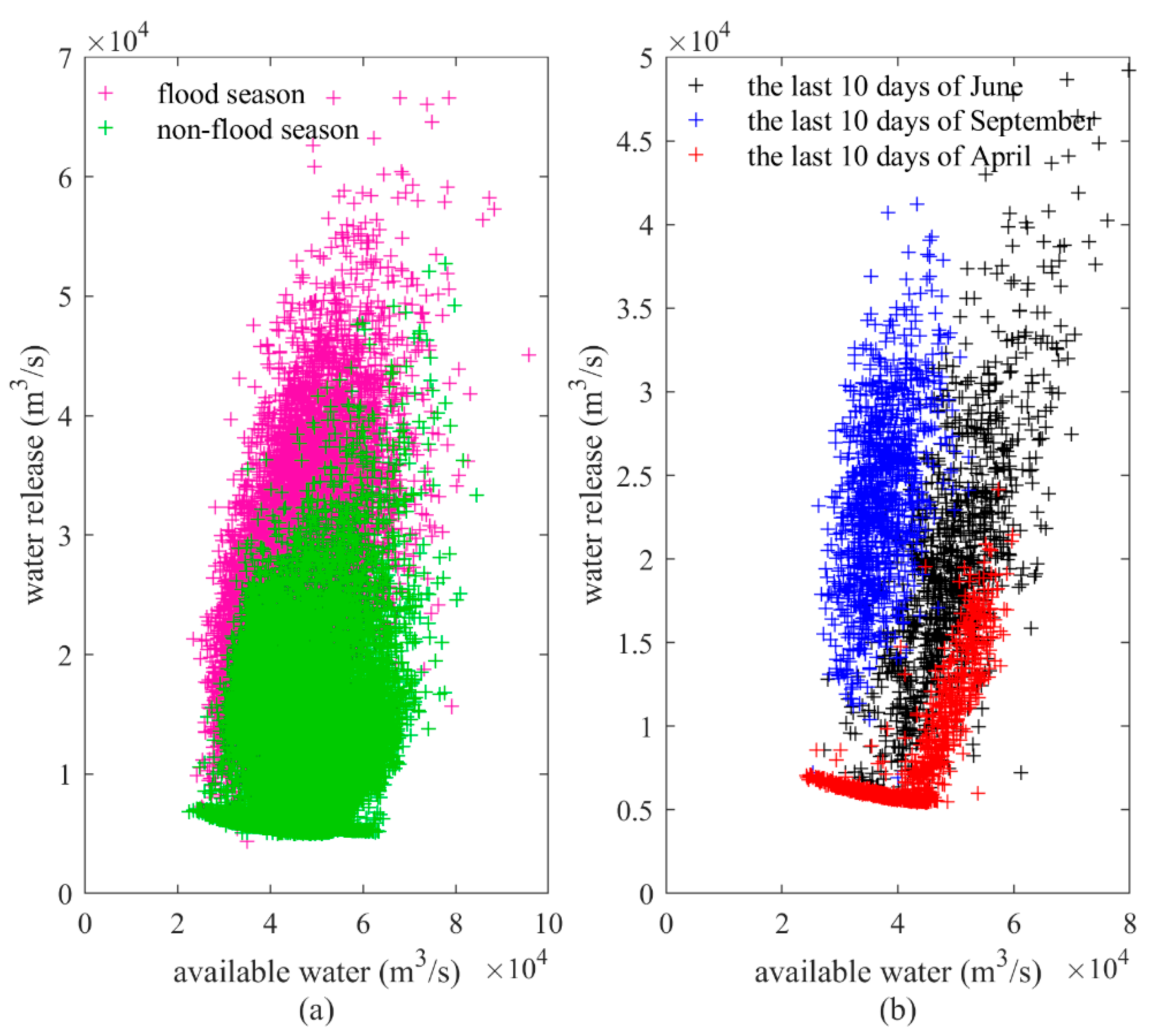
3.2.2. Optimal Solution of Deterministic Optimization Operation and Linear Operating Rules
3.2.3. Identifying the More Efficient Operating Rules Based on System Dynamics Simulation
3.3. Discussion of Results
4. Conclusions
Author Contributions
Funding
Acknowledgments
Conflicts of Interest
References
- Feng, M.; Liu, P.; Guo, S.; Gui, Z.; Zhang, X.; Zhang, W.; Xiong, L. Identifying changing patterns of reservoir operating rules under various inflow alteration scenarios. Adv. Water Resour. 2017, 104, 23–36. [Google Scholar] [CrossRef]
- Sangiorgio, M.; Guariso, G. NN-based implicit stochastic optimization of multi-reservoir systems management. Water 2018, 10, 303. [Google Scholar] [CrossRef]
- Liu, X.; Guo, S.; Liu, P.; Chen, L.; Li, X. Deriving Optimal Refill Rules for Multi-Purpose Reservoir Operation. Water Resour. Manag. 2011, 25, 431–448. [Google Scholar] [CrossRef]
- Simonovic, S. The implicit stochastic model for reservoir yield optimization. Water Resour. Res. 1987, 23, 2159–2165. [Google Scholar] [CrossRef]
- Yeh, W.G. Reservoir Management and Operations Models’. Water Resour. Res. 1985, 21, 1797–1818. [Google Scholar] [CrossRef]
- He, Z.; Zhou, J.; Mo, L.; Qin, H.; Xiao, X.; Jia, B.; Wang, C. Multiobjective Reservoir Operation Optimization Using Improved Multiobjective Dynamic Programming Based on Reference Lines. IEEE Access 2019, 7, 103473–103484. [Google Scholar] [CrossRef]
- Labadie, J.W. Optimal operation of multireservoir systems: State-of-the-art review. J. Water Resour. Plan. Manag. 2004, 130, 93–111. [Google Scholar] [CrossRef]
- Rani, D.; Moreira, M.M. Simulation-optimization modeling: A survey and potential application in reservoir systems operation. Water Resour. Manag. 2010, 24, 1107–1138. [Google Scholar] [CrossRef]
- Wurbs, R.A. Reservoir-system simulation and optimization models. J. Water Resour. Plan. Manag. 1993, 119, 455–472. [Google Scholar] [CrossRef]
- Ahmad, A.; El-Shafie, A.; Mohd Razali, S.F.; Mohamad, Z.S. Reservoir optimization in water resources: A review. Water Resour. Manag. 2014, 28, 3391–3405. [Google Scholar] [CrossRef]
- Hossain, M.S.; El-shafie, A. Intelligent Systems in Optimizing Reservoir Operation Policy: A Review. Water Resour. Manag. 2013, 27, 3387–3407. [Google Scholar] [CrossRef]
- Simonovic, S.P. Reservoir systems analysis: Closing gap between theory and practice. J. Water Resour. Plan. Manag. 1992, 118, 262–280. [Google Scholar] [CrossRef]
- He, Z.; Zhou, J.; Xie, M.; Jia, B.; Bao, Z.; Qin, H.; Zhang, H. Study on guaranteed output constraints in the long term joint optimal scheduling for the hydropower station group. Energy 2019, 185, 1210–1224. [Google Scholar] [CrossRef]
- He, Z.; Zhou, J.; Qin, H.; Jia, B.; Lu, C. Long-term joint scheduling of hydropower station group in the upper reaches of the Yangtze River using partition parameter adaptation differential evolution. Eng. Appl. Artif. Intell. 2019, 81, 1–13. [Google Scholar] [CrossRef]
- Liu, P.; Guo, S.; Xu, X.; Chen, J. Derivation of Aggregation-Based Joint Operating Rule Curves for Cascade Hydropower Reservoirs. Water Resour. Manag. 2011, 25, 3177–3200. [Google Scholar] [CrossRef]
- Feng, M.; Liu, P.; Guo, S.; Shi, L.; Deng, C.; Ming, B. Deriving adaptive operating rules of hydropower reservoirs using time-varying parameters generated by the EnKF. Water Resour. Res. 2017, 53, 6885–6907. [Google Scholar] [CrossRef]
- Young, G.K. Finding reservoir operating rules. J. Hydraul. Div. 1967, 93, 297–322. [Google Scholar]
- Aboutalebi, M.; Bozorg Haddad, O.; Loáiciga, H.A. Optimal monthly reservoir operation rules for hydropower generation derived with SVR-NSGAII. J. Water Resour. Plan. Manag. 2015, 141, 1–9. [Google Scholar] [CrossRef]
- Feng, Z.; Niu, W.; Zhang, R.; Wang, S.; Cheng, C. tian Operation rule derivation of hydropower reservoir by k-means clustering method and extreme learning machine based on particle swarm optimization. J. Hydrol. 2019, 576, 229–238. [Google Scholar] [CrossRef]
- Wei, C.C.; Hsu, N.S. Derived operating rules for a reservoir operation system: Comparison of decision trees, neural decision trees and fuzzy decision trees. Water Resour. Res. 2008, 44, 1–11. [Google Scholar] [CrossRef]
- Liu, Y.; Qin, H.; Mo, L.; Wang, Y.; Chen, D.; Pang, S.; Yin, X. Hierarchical Flood Operation Rules Optimization Using Multi-Objective Cultured Evolutionary Algorithm Based on Decomposition. Water Resour. Manag. 2019, 33, 337–354. [Google Scholar] [CrossRef]
- Liu, Y.; Qin, H.; Zhang, Z.; Yao, L.; Wang, Y.; Li, J.; Liu, G.; Zhou, J. Deriving Reservoir Operation Rule based on Bayesian Deep Learning Method Considering Multiple Uncertainties. J. Hydrol. 2019, 579, 124207. [Google Scholar] [CrossRef]
- Liu, P.; Li, L.; Chen, G.; Rheinheimer, D.E. Parameter uncertainty analysis of reservoir operating rules based on implicit stochastic optimization. J. Hydrol. 2014, 514, 102–113. [Google Scholar] [CrossRef]
- Little, J.D.C. The use of storage water in a hydroelectric system. J. Oper. Res. Soc. Am. 1955, 3, 187–197. [Google Scholar] [CrossRef]
- Celeste, A.B.; Billib, M. Evaluation of stochastic reservoir operation optimization models. Adv. Water Resour. 2009, 32, 1429–1443. [Google Scholar] [CrossRef]
- Lei, X.; Tan, Q.; Wang, X.; Wang, H.; Wen, X.; Wang, C.; Zhang, J. Stochastic optimal operation of reservoirs based on copula functions. J. Hydrol. 2018, 557, 265–275. [Google Scholar] [CrossRef]
- Stedinger, J.R.; Sule, B.F.; Loucks, D.P. Stochastic dynamic programming models for reservoir operation optimization. Water Resour. Res. 1984, 20, 1499–1505. [Google Scholar] [CrossRef]
- Tilmant, A.; Pinte, D.; Goor, Q. Assessing marginal water values in multipurpose multireservoir systems via stochastic programming. Water Resour. Res. 2008, 44, 1–17. [Google Scholar] [CrossRef]
- Lund, J.R.; Ferreira, I. Operating rule optimization for Missouri River reservoir system. J. Water Resour. Plan. Manag. 1996, 122, 287–295. [Google Scholar] [CrossRef]
- Niu, W.J.; Feng, Z.K.; Feng, B.F.; Min, Y.W.; Cheng, C.T.; Zhou, J.Z. Comparison of multiple linear regression, artificial neural network, extreme learning machine, and support vector machine in deriving operation rule of hydropower reservoir. Water 2019, 11, 88. [Google Scholar] [CrossRef]
- Li, L.; Liu, P.; Rheinheimer, D.E.; Deng, C.; Zhou, Y. Identifying Explicit Formulation of Operating Rules for Multi-Reservoir Systems Using Genetic Programming. Water Resour. Manag. 2014, 28, 1545–1565. [Google Scholar] [CrossRef]
- Ji, C.M.; Zhou, T.; Huang, H. tao Operating Rules Derivation of Jinsha Reservoirs System with Parameter Calibrated Support Vector Regression. Water Resour. Manag. 2014, 28, 2435–2451. [Google Scholar] [CrossRef]
- Liu, P.; Guo, S.; Xiong, L.; Li, W.; Zhang, H. Deriving reservoir refill operating rules by using the proposed DPNS model. Water Resour. Manag. 2006, 20, 337–357. [Google Scholar] [CrossRef]
- Forrester, J.W. Industrial Dynamics. A major breakthrough for decision makers. Harv. Bus. Rev. 1958, 36, 37–66. [Google Scholar]
- Yuan, L.; Zhou, J. Self-Optimization System Dynamics Simulation of Real-Time Short Term Cascade Hydropower System Considering Uncertainties. Water Resour. Manag. 2017, 31, 2127–2140. [Google Scholar] [CrossRef]
- Felfelani, F.; Movahed, A.J.; Zarghami, M. Simulating hedging rules for effective reservoir operation by using system dynamics: A case study of dez Reservoir, Iran. Lake Reserv. Manag. 2013, 29, 126–140. [Google Scholar] [CrossRef] [Green Version]
- Ahmad, S.; Simonovic, S.P. System dynamics modeling of reservoir operations for flood management. J. Comput. Civ. Eng. 2000, 14, 190–198. [Google Scholar] [CrossRef]
- Xu, Z.X.; Takeuchi, K.; Ishidaira, H.; Zhang, X.W. Sustainability analysis for Yellow River water resources using the system dynamics approach. Water Resour. Manag. 2002, 16, 239–261. [Google Scholar] [CrossRef]
- Jia, B.; Zhou, J.; Chen, L.; He, Z.; Yuan, L.; Chen, X.; Zhu, J. Self-optimization system dynamics simulation of reservoir operating rules. MATEC Web Conf. 2018, 246, 1937–1958. [Google Scholar] [CrossRef]
- Haase, D.; Schwarz, N. Simulation models on human-nature interactions in urban landscapes: A review including spatial economics, system dynamics, cellular automata and agent-based approaches. Living Rev. Landsc. Res. 2009, 3, 255–259. [Google Scholar] [CrossRef]
- Forrester, J.W. Industrial dynamics. J. Oper. Res. Soc. 1997, 48, 1037–1041. [Google Scholar] [CrossRef]
- Kwakkel, J.H.; Pruyt, E. Using System Dynamics for Grand Challenges: The ESDMA Approach. Syst. Res. Behav. Sci. 2015, 3, 358–375. [Google Scholar] [CrossRef]
- Sterman, J.D. Business Dynamics: Systems Thinking and Modeling for A Complex World. Irwin/McGraw Hill: Boston, MA, USA, 2000. [Google Scholar]
- Yang, J.; Lei, K.; Khu, S.; Meng, W. Assessment of Water Resources Carrying Capacity for Sustainable Development Based on a System Dynamics Model: A Case Study of Tieling City, China. Water Resour. Manag. 2015, 29, 885–899. [Google Scholar] [CrossRef]
- Li, Z.; Li, C.; Wang, X.; Peng, C.; Cai, Y.; Huang, W. A hybrid system dynamics and optimization approach for supporting sustainable water resources planning in Zhengzhou City, China. J. Hydrol. 2018, 556, 50–60. [Google Scholar] [CrossRef]
- Winz, I.; Brierley, G.; Trowsdale, S. The use of system dynamics simulation in water resources management. Water Resour. Manag. 2009, 23, 1301–1323. [Google Scholar] [CrossRef]
- Teegavarapu, R.S.V.; Simonovic, S.P. Simulation of Multiple Hydropower Reservoir Operations Using System Dynamics Approach. Water Resour. Manag. 2014, 28, 1937–1958. [Google Scholar] [CrossRef]
- King, L.M.; Simonovic, S.P.; Hartford, D.N.D. Using system dynamics simulation for assessment of hydropower system safety. Water Resour. Res. 2017, 53, 7148–7174. [Google Scholar] [CrossRef]
- Szilagyi, J.; Balint, G.; Csik, A. A Hybrid, Markov chain-based model for daily streamflow generation at multiple catchment sites. J. Hydrol. Eng. 2006, 11, 245. [Google Scholar] [CrossRef] [Green Version]
- MWR. Regulation for Calculating Design Flood of Water Resources AND Hydropower Projects. Chinese Water Resources and Hydropower Press: Beijing, China, 2006. [Google Scholar]
- Salas, J.D. Analysis and modelling of hydrologic time series. In Handbook of Hydrology; Maidment, D.R., Ed.; McGraw Hill: New York, NY, USA, 1993; Chapter 19. [Google Scholar]
- Koutsoyiannis, D.; Economou, A. Evaluation of the parameterization-simulation-optimization approach for the control of reservoir systems. Water Resour. Res. 2003, 39, 1170. [Google Scholar] [CrossRef] [Green Version]
- Bhaskar, N.R.; Whitlatch, E.E. Derivation of monthly reservoir release policies. Water Resour. Res. 1980, 16, 987–993. [Google Scholar] [CrossRef]
- Xie, M.; Zhou, J.; Li, C.; Zhu, S. Long-term generation scheduling of Xiluodu and Xiangjiaba cascade hydro plants considering monthly streamflow forecasting error. Energy Convers. Manag. 2015, 105, 368–376. [Google Scholar] [CrossRef]
- Bellman, R. Dynamic programming. Science 1966, 153, 34–37. [Google Scholar] [CrossRef] [PubMed]
- Cooperation, V. Vensim User’s Guide; Vent. Syst. Inc.: Cambridge, MA, USA, 2019; Available online: http://vensim.com/documentation/ (accessed on 20 September 2019).


| Time | Operating Rules | Rule 1 | Critical Value (m3/s) | Rule 2 | ||
|---|---|---|---|---|---|---|
| aj | bj | aj | bj | |||
| The first 10 days of January | Operating rule A | 1.00000 | −45,486.1 | 50,640 | −0.03103 | 6742.2 |
| Operating rule B | 0.01589 | 4428.9 | 50,160 | −0.02303 | 6365.6 | |
| The middle 10 days of January | Operating rule A | 1.00000 | −45,486.1 | 50,700 | −0.03231 | 6810.0 |
| Operating rule B | 0.68758 | −29,870.7 | 50,910 | −0.02608 | 6518.2 | |
| The last 11 days of January | Operating rule A | 1.00000 | −41,351.0 | 46,520 | −0.03698 | 6893.4 |
| Operating rule B | 0.17476 | −2948.9 | 46,270 | −0.03589 | 6853.8 | |
| The first 10 days of August | Operating rule A | 0.99439 | −19,586.6 | / | / | / |
| Operating rule B | 0.48547 | 4707.5 | / | / | / | |
| The middle 10 days of August | Operating rule A | 1.00000 | −19,849.5 | / | / | / |
| Operating rule B | 0.56703 | 1026.1 | / | / | / | |
| The last 11 days of August | Operating rule A | 1.00000 | −18,045.0 | / | / | / |
| Operating rule B | 0.49145 | 4454.7 | / | / | / | |
| Scheme | Average Annual Power Generation (108 kWh) | Guarantee Rate (%) | Spill Water (106 m3) |
|---|---|---|---|
| Operating rule A | 849.67 | 95.31 | 34.72 |
| Operating rule B | 846.22 | 93.06 | 34.72 |
| DP algorithm | 853.84 | 98.09 | 0 |
| Scheme | Annual Power Generation (108 kWh) | Guarantee Rate (%) | Spill Water (106 m3) |
|---|---|---|---|
| Operating rule A | 824.67 | 86.5 | 0 |
| Operating rule B | 813.99 | 86.5 | 0 |
© 2019 by the authors. Licensee MDPI, Basel, Switzerland. This article is an open access article distributed under the terms and conditions of the Creative Commons Attribution (CC BY) license (http://creativecommons.org/licenses/by/4.0/).
Share and Cite
Zhou, J.; Jia, B.; Chen, X.; Qin, H.; He, Z.; Liu, G. Identifying Efficient Operating Rules for Hydropower Reservoirs Using System Dynamics Approach—A Case Study of Three Gorges Reservoir, China. Water 2019, 11, 2448. https://doi.org/10.3390/w11122448
Zhou J, Jia B, Chen X, Qin H, He Z, Liu G. Identifying Efficient Operating Rules for Hydropower Reservoirs Using System Dynamics Approach—A Case Study of Three Gorges Reservoir, China. Water. 2019; 11(12):2448. https://doi.org/10.3390/w11122448
Chicago/Turabian StyleZhou, Jianzhong, Benjun Jia, Xiao Chen, Hui Qin, Zhongzheng He, and Guangbiao Liu. 2019. "Identifying Efficient Operating Rules for Hydropower Reservoirs Using System Dynamics Approach—A Case Study of Three Gorges Reservoir, China" Water 11, no. 12: 2448. https://doi.org/10.3390/w11122448