Analysis of the Behavior of Daily Maximum Rainfall within the Department of Atlántico, Colombia


1
School of Engineering, Civil and Environmental Engineering Master Program, Universidad Tecnológica de Bolívar, Cartagena de Indias 131001, Colombia
2
Boswell Engineering, South Hackensack, NJ 07606, USA
3
School of Engineering, Civil Engineering Program, Universidad de Cartagena, Cartagena de Indias 13001, Colombia
*
Author to whom correspondence should be addressed.
Water 2019, 11(12), 2453; https://doi.org/10.3390/w11122453
Submission received: 17 October 2019
/
Revised: 17 November 2019
/
Accepted: 19 November 2019
/
Published: 22 November 2019
(This article belongs to the Section Hydrology)
Abstract
:In the Colombian Caribbean region, there are few studies that evaluated the behavior of one of the most commonly used variables in hydrological analyses: the maximum daily rainfall (Pmax-24h). In this study, multiannual Pmax-24h time series from 19 rain gauges, located within the department of Atlántico, were analyzed to (a) determine possible increasing/decreasing trends over time, (b) identify regions with homogeneous behavior of Pmax-24h, (c) assess whether the time series are better suited under either a stationary or non-stationary frequency analysis, (d) generate isohyetal maps under stationary, non-stationary, and mixed conditions, and (e) evaluate the isohyetal maps by means of the calculation of areal rainfall (Pareal) in nine watersheds. In spite of the presence of both increasing and decreasing trends, only the Puerto Giraldo rain gauge showed a significant decreasing trend. Also, three regions (east, central, and west) with similar Pmax-24h behavior were identified. According to the Akaike information criterion test, 79% of the rain gauges showed better fit under stationary conditions. Finally, statistical analysis revealed that, under stationary conditions, the errors in the calculation of Pareal were more frequent, while the magnitude of the errors was larger under non-stationary conditions, especially in the central–south region.
1. Introduction
Globally, changes in the pattern of behavior of hydrometeorological variables (e.g., precipitation, temperature, runoff, relative humidity, etc.) are influenced, among others, by population growth, watershed land-use/land-cover (LULC) changes, and the increase in greenhouse gases emissions [1,2]. In Colombia, the Institute of Hydrology, Meteorology, and Environmental Studies (IDEAM, in Spanish) conducted several studies focused on evaluating the changes in the behavioral patterns of some hydrometeorological variables [3,4,5,6,7]. IDEAM [3] analyzed the annual average rainfall trend over the periods 2011–2040, 2041–2070, and 2071–2100 for the different departments (political and administrative territorial units) that compose the five regions of Colombia (Caribbean, Pacific, Andean, Orinoco, and Amazon). According to the study, the department of Atlántico (located within the Caribbean region) will experience an annual average rainfall decrease ranging from 7.39% through 11.26% during the 2011–2100 period. In addition, it was predicted that some of the municipalities located in the southeast of the department will be the most affected.
Such changes in the hydrological cycle can lead to (a) decreases in the water supply (both for human consumption and for the different sectors of the economy), (b) possible water supply cost increase, and (c) under- or oversized hydraulic structures for stormwater management [8]. Several studies analyzed the rainfall behavior within the department of Atlántico [9,10,11,12,13]. However, none analyzed the maximum daily rainfall (Pmax-24h) time series trends or whether they (the trends) have regional behavior within the department. González-Álvarez et al. [14] detected increasing and decreasing linear trends in some of the multiannual Pmax-24h time series of the 13 rain gauges analyzed in the department of Atlántico, which further suggested the presence of non-stationarity. Despite the findings, the scope of the study did not cover a detailed analysis of trends using non-parametric tests (e.g., Mann–Kendall and Spearman’s rho) and the possible presence of different regions exhibiting similar rainfall behavior. Furthermore, the study did not determine whether a non-stationary frequency analysis was more convenient than a stationary one when estimating the Pmax-24h associated with the different return periods and their possible impact on (a) the isohyetal alignments, and (b) the subsequent computation of the areal rainfall of a given watershed.
Several municipalities, within the department of Atlántico, experience different affectations that go from severe and prolonged droughts [15] to more recurrent and devastating floods [13,16,17]. During the rainy season of 2010–2011, a great portion of the southern part of the department was flooded, causing a dyke breakage that exacerbated the problem with 185,236 people affected and total losses (infrastructure, habitat, etc.) estimated to be approximately United States dollars (USD) $491 million, of which infrastructure accounted for 11% [18]. All these extreme events could indicate a change in the rainfall regime (particularly Pmax-24h) that needs to be analyzed, especially for the design of stormwater management infrastructure. Thus, this study uses multiannual time series of Pmax-24h from 19 rain gages within the department of Atlántico to (a) analyze the time series trends by means of the Mann–Kendall (MK), Spearman’s rho (SR), and Theil–Sen estimator as a first step to identify possible changes in the rainfall pattern over time, (b) determine and delineate regions with homogeneous Pmax-24h behavior, which contributes to the understanding of rainfall behavior mainly in ungauged areas, (c) perform both a stationary and a non-stationary rainfall frequency analysis in order to calculate Pmax-24h for return periods of five, 10, 25, 50, and 100 years, (d) determine, via Akaike information criterion (AIC) test, whether a stationary or a non-stationary frequency analysis better fits the time series analyzed, and (e) draw isohyetal maps for different return periods by using the Pmax-24h under both stationary and non-stationary conditions, as well as mixed (stationary and non-stationary Pmax-24h based on the AIC test results), so as to evaluate the possible implications of not taking into account pattern shifts observed in a variable such as Pmax-24h commonly used in water resource-related projects (e.g., flood risk evaluation, design of hydraulic structures for stormwater management, water balances, and water scarcity, among others). Ultimately, the findings herein are intended to show the importance of adapting those projects to climate changes through a thorough analysis that permits a better understanding of the hydrological variables as part of the decision-making process.
2. Study Area and Data
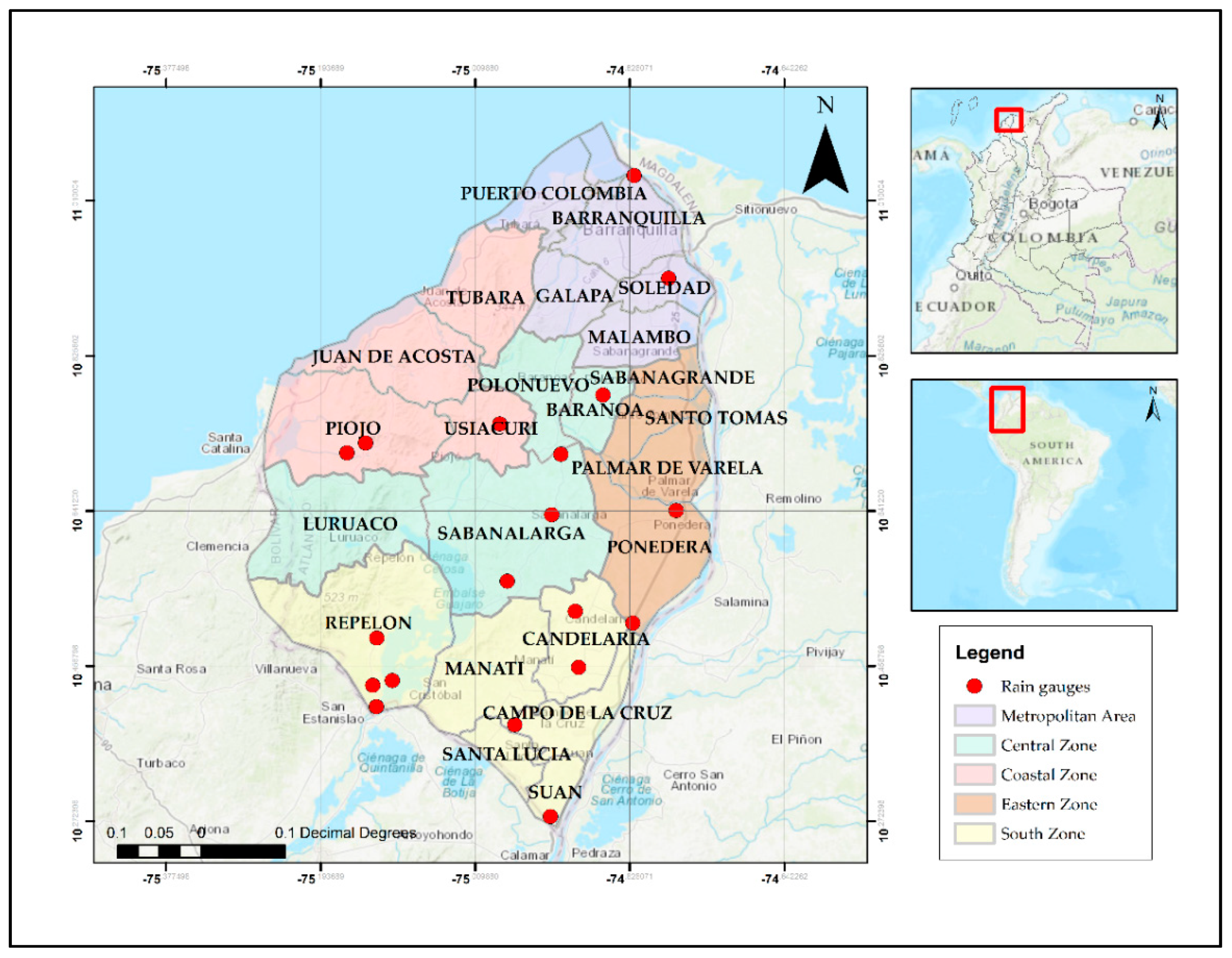
The department of Atlántico, located in the Caribbean region, is one of the 32 departments into which Colombia is politically divided [19,20]. This department has an area of 3386 km2 and consists of 23 municipalities, grouped into five regions: Metropolitan Area, Coastal, Eastern, Central, and South (Table 1 and Figure 1) [21].
The department of Atlántico has a warm and dry climate, with an average annual temperature of approximately 28 °C and maximum temperatures that can reach up to 40 °C. The average annual rainfall ranges from 500 mm to 1500 mm [15]. The rainfall regime has three seasons: dry (December to March), transition (late April to June), and rainy (August to early December) [22].
In this research, multi-annual series of maximum daily rainfall were used, from 19 rain gauges operated by IDEAM (Table 2), totaling 728 observations from 1940 to 2015 (records from 2016–2019 were not included as some rain gauges do not yet have the information available for those years). The rain gauges used in this study were selected under the following criteria: (a) time series with a minimum of 20 years of data, (b) exclusion of rain gauges with less than 25% of the rainfall information in any given year, (c) exclusion of rain gauges that did not have information from the months corresponding to the rainy season [23], and (d) elimination of outliers by means of the Water Resources Council method [24]. The selected rain gauges are shown in Table 2.
3. Methodology
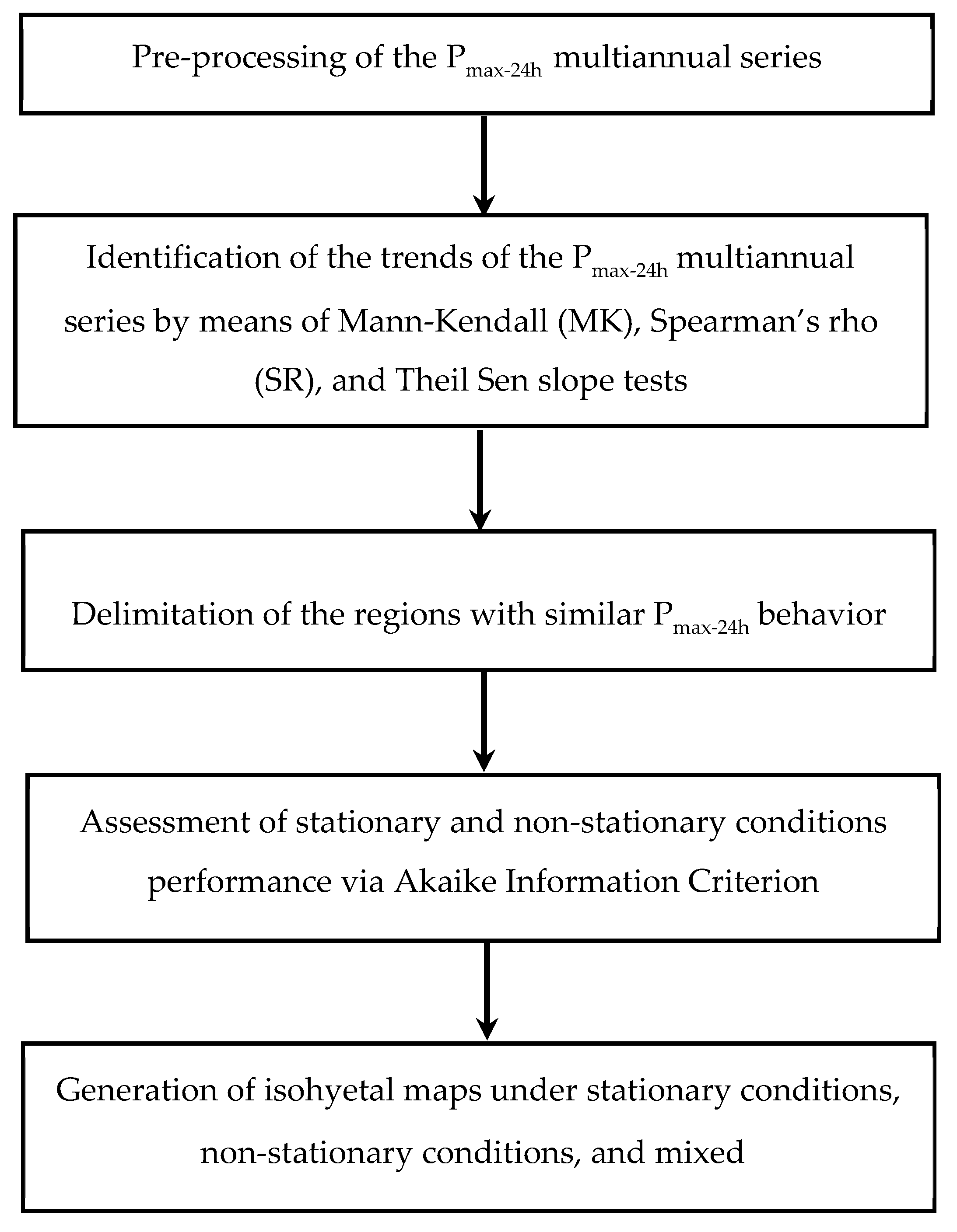
After selecting the rain gauges that met the abovementioned criteria, the rainfall time series underwent further analysis. Figure 2 shows the steps that make up the methodology proposed in this research.
3.1. Trend Analysis
In this study, the monotonic trend detection was performed through the nonparametric tests of Mann–Kendall and Spearman’s rho [25], with a significance level of 5%. Nonparametric testing has the advantage of being able to detect trends, independently of whether the data has a normal distribution or not, as with hydrometeorological variables [26]. In addition, the analysis was complemented by determining the magnitude of the trends’ slopes identified in the Pmax-24h series using the Theil–Sen slope [27].
3.1.1. Mann–Kendall (MK) Test
The test considers a null hypothesis (H0) when no trend (to increase or decrease) exists and an alternative hypothesis (H1) that there is a trend. The calculation of Mann–Kendall’s statistics S and standardized Z uses the following set of formulas (Equation (1)):
where Xi and Xj represent the time series data in chronological order, n is the number of data points in the time series, tp is the number of links for the p-th value, and q is the number of links. Positive Z values (MK statistic) indicate the presence of increasing trends, and negative values indicate decreasing trends. If |Z| > Z1 − α/2, the null hypothesis is rejected, indicating a statistically significant trend. The critical value of Z1 − α/2 for a significance level of 5% is 1.96 [26]. That is, a trend is considered increasing or decreasing, at a significance level of 5%, only if ZMK is greater than |1.96|. Otherwise, it is considered trendless (constant).
3.1.2. Spearman’s Rho (SR) Test
This test assumes that the data are independent and identically distributed. Null and alternative hypotheses are defined the same way as in the Mann–Kendall test [28]. The RSR and ZSR statistical variables are calculated using Equations (2) and (3).
where Di represents the i-th observation, i is the chronological order of the number, n is the number of observations, ZSR is the value of the t-student distribution with n − 2 degrees of freedom. Positive and negative ZSR values represent increasing and decreasing trends, respectively. If |ZSR|> t(n−2,1−α/2), the null hypothesis is rejected, demonstrating statistically significant trends [10,29].
3.1.3. Estimator of Theil–Sen Slope
This estimator allows determining the actual slope of the trends of a given time series. The principle of this estimator is based on the assumption that, when a series of data shows a linear trend, the median of the slope of the linear trend can be calculated using the slopes of several data points, and this value represents the slope of its trend (Equation (4)) [30,31].
where βTS represents the slope between the xj and xk points in the time series (which corresponds to the time points j and k, with j > k).
3.2. Delimiting Homogeneous Regions
The delimitation of regions with similar hydrometeorological conditions involved a statistical analysis of the data observed in the study area [32,33] by means of the regionalization method suggested by Hosking and Wallis [34]. This method defines statistical parameters similarly to the traditional L-moments, which, in turn, involves the calculation of the β estimators (Equations (5)–(8)).
where Xi represents the value of the Pmax-24h series, i is the rank of each data point arranged from highest to lowest, and n is the number of data points in the series of each rain gauge j. Subsequently, the L-moments (represented with λ) are obtained using Equations (9)–(12).
Finally, the dimensionless L-moments were calculated using Equations (13)–(15), where τ2 represents the coefficient of variation, τ3 is the asymmetry coefficient, and τ4 is the kurtosis coefficient.
Homogeneous regions were then formed via cluster analysis by means of the K-means method [35], which allows the dimensional L-moments to be related to the elevation and location parameters of each of the rain gauges. This way, the clusters sharing similar characteristics are detected so that the homogeneous regions can be defined. Additionally, varying the number of clusters in the K-means method helps with finding a geographically consistent configuration. Finally, the selected cluster configuration was reassessed using the methodology used by Hosking et al. [36] in order to corroborate the region’s homogeneity.
3.3. Stationary and Non-Stationary Rainfall Frequency Analysis
The point rainfall values used for the Pmax-24h isohyetals were estimated via frequency analysis for both stationary (SC) and non-stationary (NSC) conditions for return periods of five, 10, 25, 50, and 100 years.
Based on the results obtained by González-Alvarez et al. [14] for the Colombian Caribbean region, generalized extreme value (GEV) [37] (Equation (16)) and Gumbel [38] (Equations (17)–(19)) were used for the stationary frequency analysis. The theoretical basis for these two cumulative distribution functions (CDF) can be widely found in the literature [39,40,41]. In Equations (17)–(19), k is the shape parameter, β is the mode (or location), and α is the scale (always greater than zero). GEV can take one of three extreme value (EV) distributions depending on the value of k: (a) if k equals zero, it takes the form of Type 1 EV (Gumbel); (b) if less than zero, it takes the form of Type 2 (Fréchet); (c) it takes the form of Type 3 (Weibull), if greater than zero. The Pmax-24h value selected for the stationary frequency analysis was the one that came from the function showing the best chi-square test [42] result.
The non-stationary frequency analysis was performed according to the methodology proposed by Obeysekera and Salas [1,43,44], which uses (a) the GEV function by varying the location parameter over time and maintaining the constant parameters of scale and shape (called GEVmu), and (b) a definition of the return period (Tr) according to the geometric distribution given by Equation (20), where Pj is the is the time-varying exceedance probability, and j represents the year to be projected [1,45]. The GEVmu function was already tested by Gonzalez-Alvarez et al. [45] in the Colombian Caribbean region, where a sensitivity analysis showed that varying the shape and/or scale parameters did not bring any improvement in the performance of either GEV or Gumbel distributions.
Subsequently, a linear trend model of each parameter (location, shape, and scale) was defined to estimate its value using a code programmed in the R software (Version 3.3.1, R Development Core Team, Auckland, New Zealand) with the library nsextremes [46].
After the Pmax-24h values were calculated for stationary and non-stationary conditions, the Akaike information criterion (AIC) goodness-of-fit test [47] was used to determine which of the two conditions (stationary and non-stationary) better represented the multiannual series for each of the rain gauges analyzed. The Pmax-24h values for SC, NSC, and the better of the two conditions were later used for the generation of the stationary, non-stationary, and mixed isohyetal maps, respectively (Section 3.4).
3.4. Generation of Isohyetals Maps
After obtaining the Pmax-24h values (for stationary and non-stationary conditions) for each of the rain gauges, three different types of Pmax-24h isohyetals (for return periods of five, 10, 25, 50, and 100 years) were generated (Table 3), using ArcGIS (Version 16.1, ESRI Inc., Redlands, CA, USA). For this, the inverse distance weighting (IDW) interpolation method with manual adjustment was utilized, based on the findings of González-Álvarez et al. [14] for the Colombian Caribbean region (inputs: Z-value = 2; cell size = 0.021; search radius variable, and number of points = 12).
3.5. Evaluation of the Different Isohyetal Maps
The performance of the isohyetal maps was tested in nine watersheds (three watersheds per homogeneous region) by estimating their corresponding areal precipitation under SC, NSC, and mixed conditions for return periods of five, 10, 20, 50, and 100 years. The selected watersheds had various sizes and were located at different distances from the nearest rain gauge.
After estimating the areal Pmax-24h of each of the watersheds, a statistical analysis was performed using the relative error percentage (REr) (Equation (21)), root-mean-squared error (RMSE) and standard deviation ratio (RSR) (Equation (22)), the bias percentage (PBIAS) (Equation (23)), and the Nash–Sutcliffe efficiency (NSE) (Equation (24)) [14,48,49,50,51].
REr measures the error percentage between the true and simulated values; its optimal value is zero. RSR also evaluates the error, with an optimal value of zero; however, it does so in a standardized manner by dividing the root-mean-square error (RMSE) of the true and simulated values by the standard deviation. PBIAS estimates the bias as a percentage, with an optimal value of zero; negative values indicate overestimation, while positive values indicate underestimation. NSE is an indicator of the predictive power of a model (range of values from −∞ to one); it measures how the simulated values resemble true values (dispersion around the 1:1 line). The optimal value of NSE is one (perfect fit). Negative values indicate that it is better to use the average of true values than simulated values. Values of zero (or close to zero) indicate that either the average of true values or the simulated values could be used.
For this study, areal Pmax-24h values from the mixed isohyetals were assumed to be the true value, given that these (the isohyetals) were derived from the point Pmax-24h data of the distribution functions that performed best according to the AIC test. In Equations (21)–(24), Ptrue represents the true areal Pmax-24h, Psim corresponds to the areal Pmax-24h estimated from both the stationary and the non-stationary isohyetals, n is the number of watersheds analyzed, and i is the watershed analyzed.
4. Results and Discussion
4.1. Trend Detection
The results of the MK and SR tests (Table 4) showed that only the Pmax-24h time series of the Puerto Giraldo rain gauge (gray cell in Table 4) had a significant trend at a 5% level of confidence (gray cell in Table 4). The Theil–Sen slope value of −0.89 corroborated the results obtained from the MK and SR tests.
Despite the fact that Puerto Giraldo was the only rain gauge with a significant trend, there were also other rain gauges with either increasing or decreasing trends. Out of the 19 rain gauges, 10 showed increasing trends, five of which had ZMK values greater than one. Likewise, eight rain gauges had decreasing trends, three of them with values below one. The trends of these time series, although currently considered as not significant (values less than |1.96|), should be evaluated in the coming years to determine any increment of the estimated values. With respect to the Theil–Sen slope results, San José and Hda El Rabón had values less than one. These two rain gauges are both located in the southern part of the department, where IDEAM [3] predicted a rainfall decrease. These findings help with (a) a better understanding of the rainfall regime (both annual and daily maximum), and (b) confirming the hypothesis raised by González-Álvarez et al. [37] as to the existence of Pmax-24h trends within the Colombian Caribbean coast.
4.2. Identification and Delimitation of Homogeneous Regions
Table 5 presents the results of the dimensionless L-moments τ2, τ3, and τ4 for each of the rain gauges analyzed, which were used for identifying the homogeneous regions.
Subsequently and with the purpose of defining the best homogeneous region, the K-means method was performed using clusters with different set-ups of rain gauge groups. Groups of three, four, and five clusters were defined with respect to the homogeneity presented in the variables shown in Table 5. Finally, the best configuration was selected using (a) the Hosking et al. [36] methodology, and (b) a geographical comparison among the homogeneous group distributions.
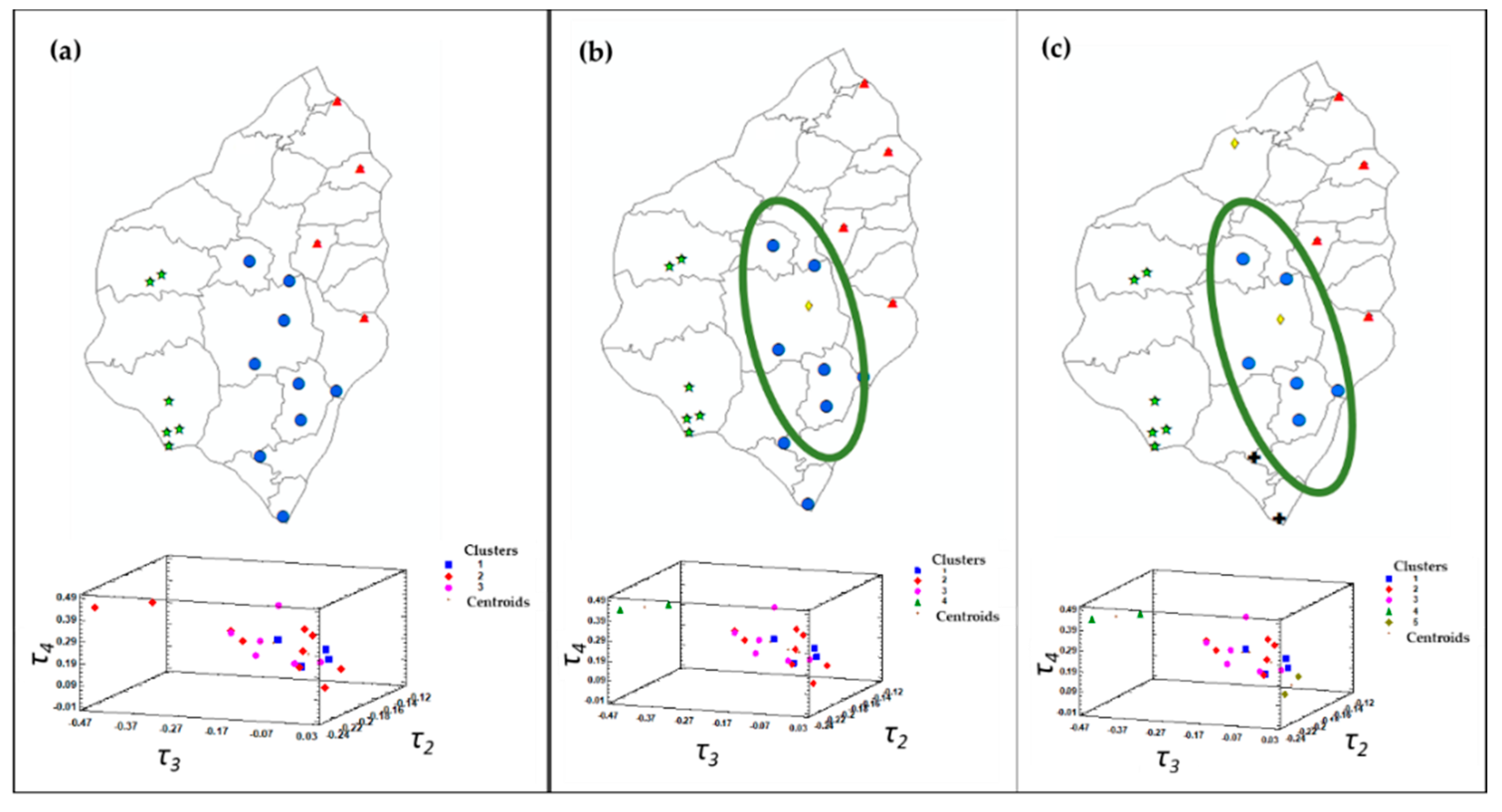
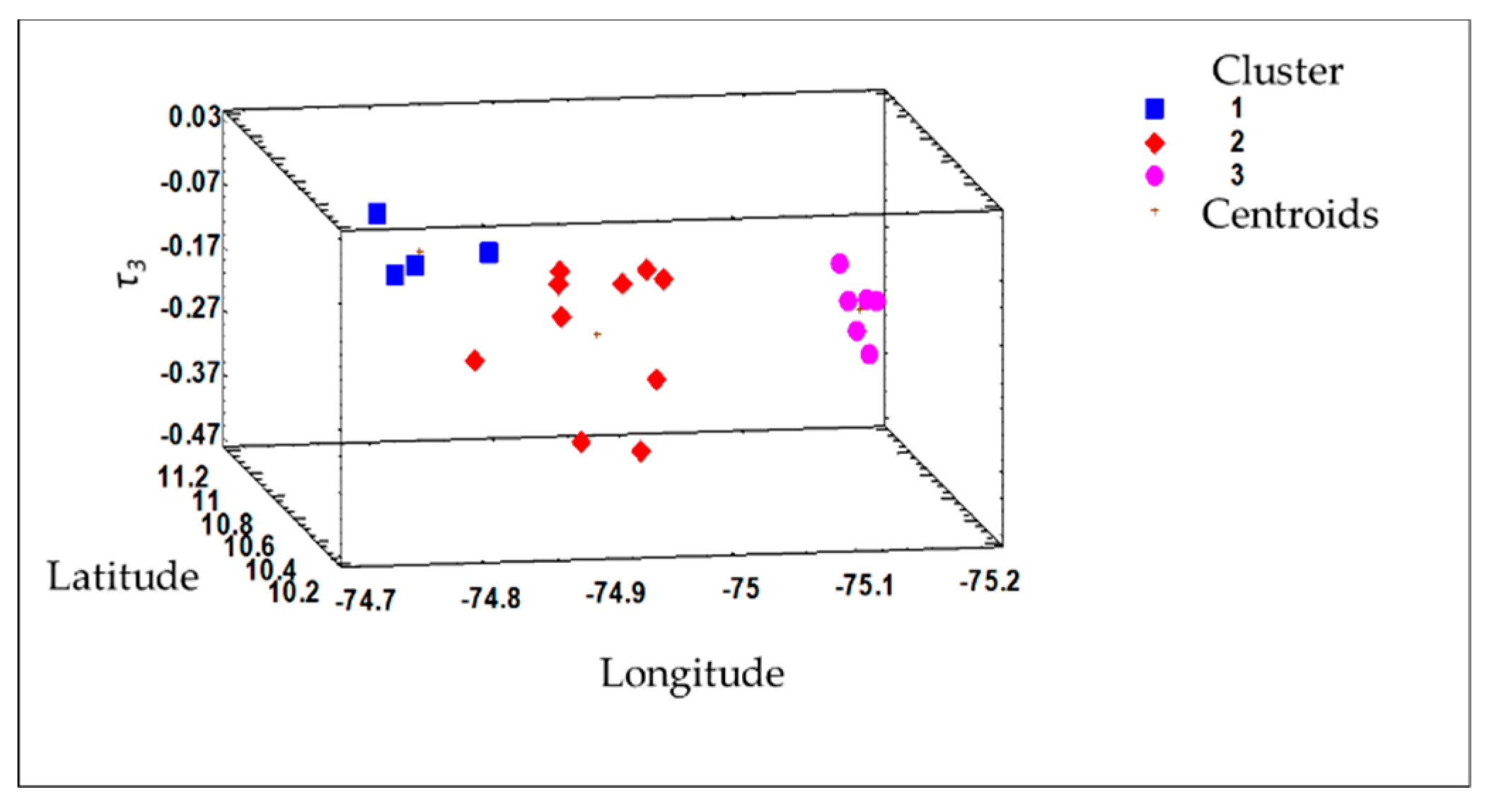
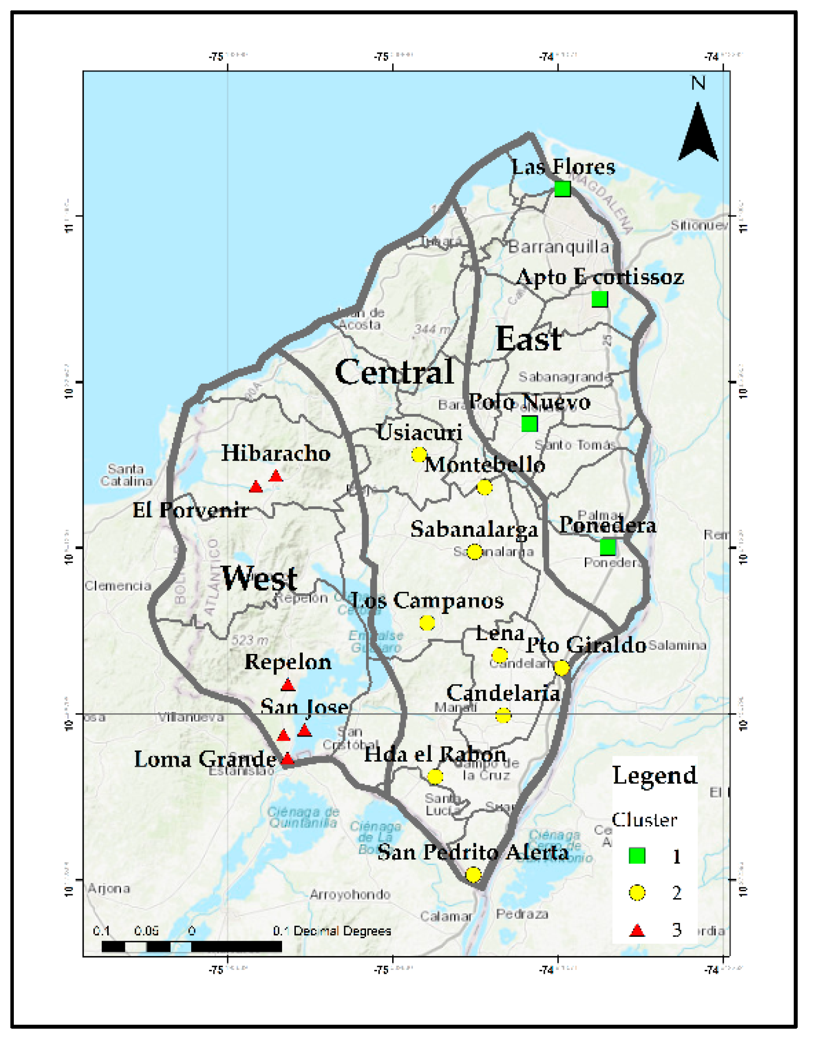
Figure 3a–c depict the rain gauge spatial distribution grouped into three, four, and five clusters, respectively. In Figure 3b,c, the green ovals show how a rain gauge belonging to another group (yellow diamond) is within a different cluster (blue circles). This indicates that grouping rain gauges into either a four- or five-rain-gauge cluster introduces geographically inconsistent distributions. In fact, Hosking et al. [37] affirmed that these types of plots (those that relate τ2, τ3, and τ4) can sometimes contain overlapping groups, which makes it difficult to select the number of clusters that adequately represent rain gauges with similar characteristics. The three-rain-gauge cluster group (Figure 3a) did not show that problem. Also, the adequacy of the three-rain-gauge cluster was further verified by analyzing the behavior of the geographic location variables (latitude and longitude) with respect to the coefficient asymmetry (τ3). Figure 4 evidences three well-defined clusters, which represent those rain gauges with similar characteristics.
4.3. Rain Frequency Analysis
4.3.1. Stationary Frequency Analysis
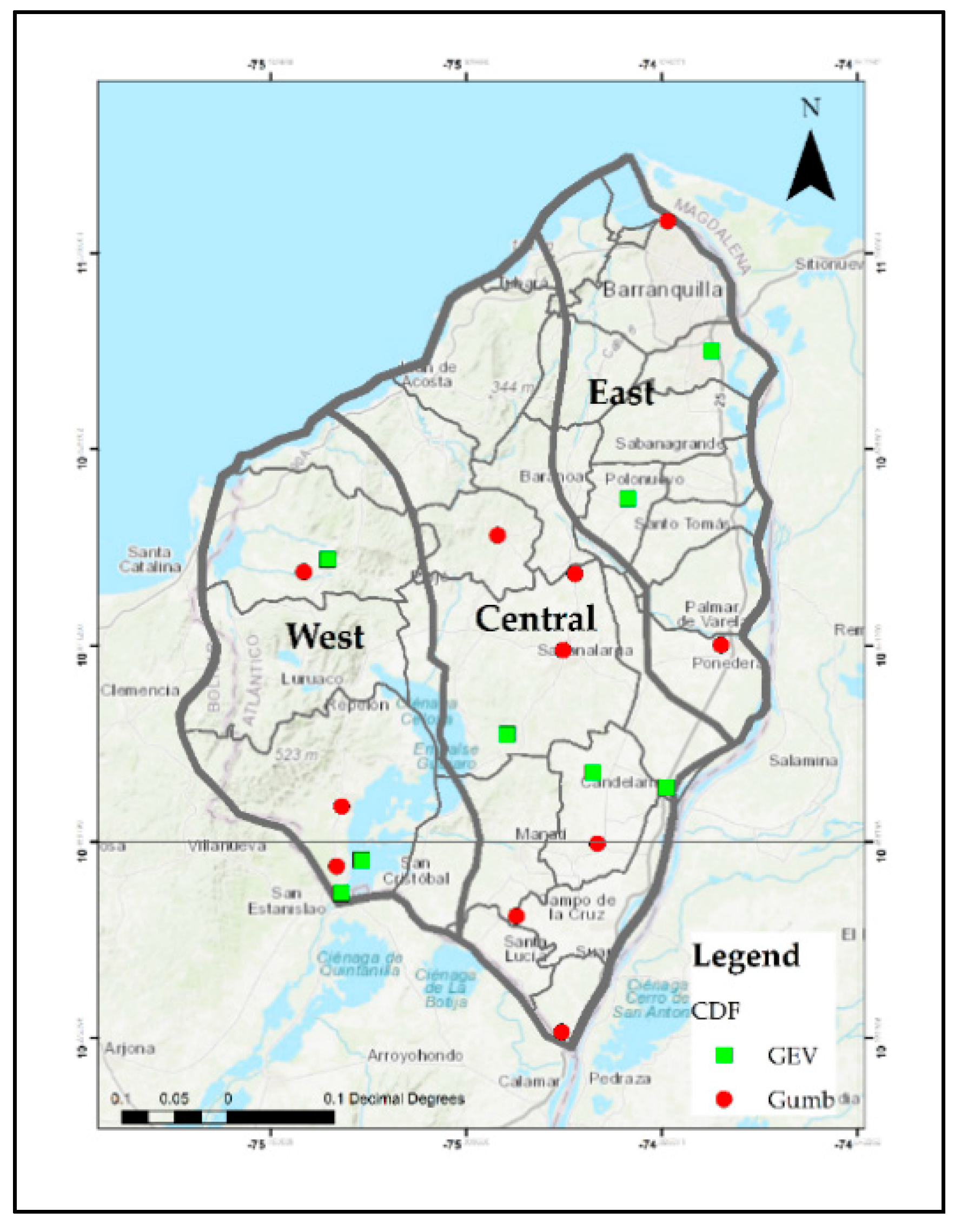
Table 7 and Figure 6 show the rain gauges (in each of the regions) where CDFs Gumbel and GEV better represented the time series. Overall, the Gumbel distribution was the best fit in 63.2% of the 19 rain gauges analyzed, while GEV was the best fit in only 36.8%. These results represent a shift from the findings by González-Álvarez et al. [45], where GEV was best in 53.8% of the 13 rain gauges assessed. This is due to the fact that the Gumbel distribution was the best CDF among the new additional six rain gauges analyzed in this study. Based on the findings and despite the fact that the Gumbel distribution was best in the majority of the cases, there was not a unique CDF that better represented all the time series within a particular region. Pmax-24h values under stationary conditions for each of the 19 rain gauges are presented in Table A1 (Appendix A).
4.3.2. Non-Stationary Frequency Analysis
Pmax-24h estimates under non-stationary conditions (by means of the GEVmu distribution) for the 19 rain gauges are compiled in Table A1 (Appendix A). Differences of up to 58.9 mm were observed at the El Porvenir rain gauge between the Pmax-24h values under stationary and non-stationary conditions for a 100-year return period.
4.3.3. Selecting the Best Pmax-24h Value
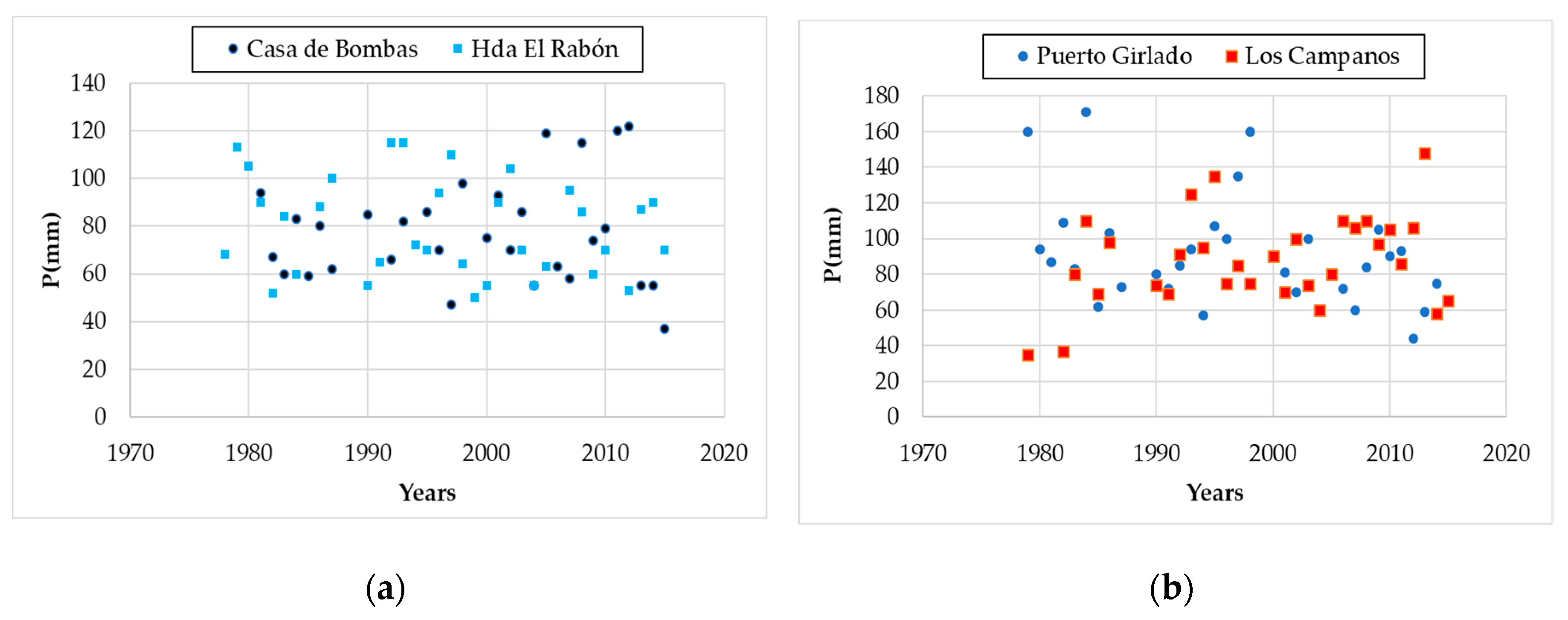
After the estimation of the Pmax-24h under both stationary and non-stationary conditions, it was necessary to determine—via AIC test—which of the two conditions better represented the time series (Table 8). The values obtained in this section were later used for the generation of isohyetal maps called mixed (derived from the best rainfall value of the two conditions) explained in the next section. Table 8 shows the best condition (stationary or non-stationary) and CDF, as well as the AIC test values obtained. Figure 7 depicts the time series of rain gauges at Casa de Bombas, Hda El Rabón, Puerto Giraldo, and Los Campanos. For the first two rain gauges, a stationary condition frequency analysis is best, according to the AIC test, while the last two suit a non-stationary one.
4.4. Isohyetal Maps
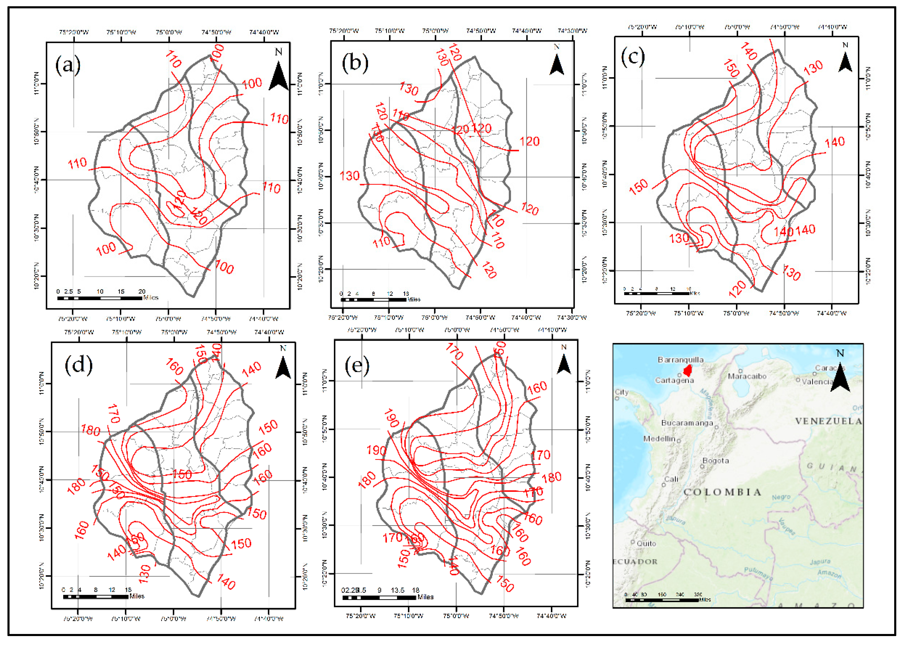
With the Pmax-24h values of the 19 rain gauges obtained in Section 4.3.1, Section 4.3.2, Section 4.3.3, maps of stationary (Figure 8), non-stationary (Figure 9), and mixed (the best value of the two conditions according to the AIC test, Figure 10) isohyetals were drawn for return periods of five, 10, 25, 50, and 100 years.
Figure 8 shows that isohyetal values ranged from 100–110 mm for five years, from 110–120 mm for 10 years, from 120–150 mm for 25 years, from 130–160 mm for 50 years, and from 140–180 mm for 100 years.
Figure 9 shows values of 90–120 mm for a return period of five years, 100–130 mm for 10 years, 110–160 mm for 25 years, 110–180 mm for 50 years, and 110–210 mm for 100 years.
Finally, in Figure 10, it can be observed that the isohyetals ranged from 100–120 mm for five years, from 110–130 mm for 10 years, from 120–150 mm for 25 years, from 130–180 mm for 50 years, and from 140–190 mm for 100 years. The highest values were observed in the south zone and the lowest values were observed in the north.
4.5. Isohyetal Map Assessment
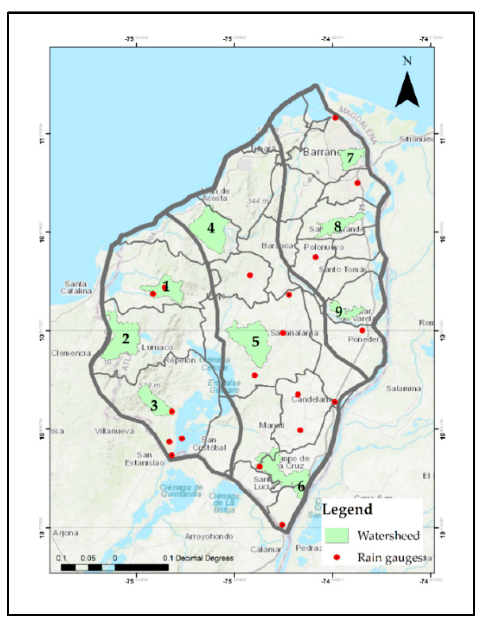
In order to assess how the use of stationary and/or non-stationary isohyetal maps could affect the calculation of the areal Pmax-24h (Pareal) in a given watershed (W), nine watersheds were selected, three in each of the three homogeneous regions (light-green areas in Figure 11). W1, W2, and W3 are located in the north, central, and southern areas of the west homogeneous region, respectively. W4, W5, and W6 are within the central region, located in the northern, central, and southern areas, respectively. Finally, W7 (north), W8 (center), and W9 (south) are located within the east region. Table 9 summarizes the watershed area, the nearest rain gauge, and its distance to each of the watersheds.
Pareal values for all watersheds (return periods of five, 10, 25, 50, and 100 years) for stationary and non-stationary conditions, as well as mixed ones, are shown in Table 10. Likewise, stationary and non-stationary Pareal values were compared, through their differences (mixed minus the SC and NSC values), with Pareal values of mixed isohyetal maps (Table 10).
Pareal values of the mixed isohyetals for the five-year return period were in a range of 95.0 mm (W3) to 109.2 mm (W8). For the 10-year return period, the value range was between 107.6 mm (W3) and 126.7 mm (W2). For the 25-year return period, values ranged from 127.3 mm (W3) to 145.5 mm (W2). For the return period of 50 years, the range was between 141.2 mm (W3) and 168.9 mm (W2). For the 100-year return period, values ranged from 153.1 mm (W3) to 179.2 mm (W5).
Pareal values of the stationary isohyetals for the five-year return period were in a range of 100.0 mm (W5) to 109.4 mm (W9). For the 10-year return period, the minimum and maximum values were between 113.0 mm (W3) and 124.2 mm (W2). For the 25-year return period, values ranged from 124.7 mm (W7) to 147.7 mm (W2). For the 50-year return period, the value range was between 135.0 mm (W7) and 160.0 mm (W2). For the 100-year return period, values ranged from 143.1 mm (W8) to 180.0 mm (W2).
Pareal values of the non-stationary isohyetals for the five-year return period were in a range of 94.8 mm (W6) to 117.7 mm (W5). For the 10-year return period, the value range was given between 101.6 mm (W6) and 125.0 mm (W9). For the 25-year return period, values ranged from 115.4 mm (W6) to 145.5 mm (W2). For the 50-year return period, values ranged from 120.1 mm (W6) to 161.7 mm (W5). For the 100-year return period, the values were between 126.8 mm (W6) and 187.0 mm (W2).
The frequency analysis under stationary conditions is most commonly used by hydrologists to estimate the design rainfall for hydraulic structures for stormwater management. Nonetheless, the differences observed in Table 10 show that the stationary frequency analysis underestimated the values of areal Pmax-24h for the study area. This behavior occurred in 60% of the cases evaluated (27 out of 45) throughout the department of Atlántico. This implies that, if a designer decides to use a stationary design rainfall, the subsequent estimation of the design flow for a given hydraulic structure could end up as an underestimated value. It can also be observed that these underestimations reach their most critical values within the central region, where the highest areal Pmax-24h differences range from 11.3 to 24.2 mm (both in W5) for return periods of 25, 50, and 100 years (which are the most used in the design of drainage hydraulic structures). The west region exhibited only two cases where the difference in Pareal had values greater than 5 mm (7.7 mm in W1 and 8.9 mm in W2). In the eastern region, underestimations occurred in 60% of cases (six cases out of 10) with values ranging from 6.8 to 11.2 mm (W7 and W8). Like the central region, these values came from return periods of 25, 50, and 100 years. These results also show that, for stationary conditions, the probability of underestimating the values of Pareal is higher in these three return periods, with values of 66%, 88%, and 66%, respectively. Rainfall differences with values less than 5 mm occurred in 57.8% of the cases (26 cases distributed as follows: nine for the west region, nine for the east region, and eight for the central region, where two values of 5.1 mm were given that could be considered within the rank).
For the non-stationary scenario, the tendency to underestimate Pareal occurred in 46.7% of the cases (21 out of 45): seven cases for the west region, nine for the central region, and five for the east region. It was also noted that, for this scenario, more Pareal values with differences less than or equal to 5 mm are estimated, which was observed in 66.7% of the cases (11 for the west region, nine for the central region, and 10 for the eastern region). On the other hand, when each of the regions was analyzed individually, the western region showed a slight tendency to overestimate the Pareal values (eight out of 15, negative values in red in Table 10). This behavior was more noticeable for the 100-year return period, where the three watersheds evaluated presented values ranging from 2.2 mm (W2) to 13.3 mm (W3). In the central region, underestimated values of Pareal (60% of the cases or nine out of 15) were observed, particularly in the southern part of this region (W6), with values ranging from 11.1 to 26.5 mm for return periods 10, 25, 50, and 100 years. For the eastern region, there was also a tendency to overestimate the Pareal (66.7% of the cases, 10 of 15), with values ranging from 2.1 mm (W9) to 19.5 mm (W8).
Regarding the real values of Pareal (mixed isohyetals), the southern area of the department of Atlántico exhibited the lowest values, specifically in W3 (located in the south of the west region) and W6 (located in the south of the eastern region). This is clearly evident, for example, when comparing the Pareal values for the 100-year return period between W6 and W7 (located northeast). W6, despite having an area three times larger than W7, has a lower Pareal value (153.3 mm versus the 155.0 mm for W7). These results coincide with the findings of IDEAM [3], who determined that municipalities located in the southeast of the department will likely be the most affected by rainfall decrease.
The isohyetal map (stationary and non-stationary) performance assessment within each of the watersheds was carried out through the relative error percentage (REr). Additionally, the performance of each of the regions was assessed by RSR, PBIAS, and NSE. The results of this statistical analysis are presented in Table 11.
For the stationary isohyetal maps, REr values ranged from 0.00% (W2) to 9.52% (W3) for the five-year return period, 0.77% (W6) to 6.17% (W4) for the 10-yearperiod, 0.13% (W3) to 8.84% (W5) for the 25-year period, 0.17% (W6) to 9.59% (W5) for the 50-year period, and 0.23% (W9) to 15.64% (W5) for the 100-year period. The highest REr values were observed in two of the return periods (50 and 100 years) most commonly used in the design of hydraulic structures for runoff management (50 and 100 years). No relationship was observed between the watershed area and REr.
For non-stationary isohyetal maps, REr values ranged from 0.00% (W3) to 4.66% (W4) for the five-year return period, 0.00% (W7) to 10.93% (W6) for the 10-year period, 0.23% (W2) to 12.10% (W6) for the 25-year period, 0.93% (W3) to 18.28% (W6) for the 50-year period, and 1.36% (W1) to 20.85% (W6) for the 100-year period. The highest REr values were observed in return periods of 50 and 100 years.
In general, for stationary conditions, there were 14 cases where REr was greater than or equal to 5.00% (gray cells). The maximum value was 15.64%, with only one case where REr was greater than or equal to 10%. For the non-stationary conditions, 10 cases were observed where the REr was greater than or equal to 5.00%. The maximum value was 20.85%, with five cases where REr was greater than or equal to 10%. Furthermore, when the stationary and non-stationary conditions were compared one-to-one, it was observed that, in 57.8% of the cases (26 out of 45), the REr values for the non-stationary conditions were lower than their stationary counterparts. These results suggest that (a) the error might be more frequent when using the stationary condition isohyetal maps, and (b) additional attention should be paid during the design of hydraulic structures under stationary frequency analysis, especially as it was also found that this scenario tends to underestimate the Pareal (Table 10).
With respect to the overall performance of all regions, the stationary conditions resulted in lower values of RSR (10 in total) than those for the non-stationary conditions (five in total). At first glance, this may indicate less error under stationary conditions (which contradicts the results previously obtained when the REr was analyzed for each watershed). Nonetheless, a closer look at Table 10 revealed that, despite the fact that each condition had five REr values greater than or equal to 5.00%, the non-stationary condition had REr values of up to 20.85%, which contributed to having an overall larger RSR value. Such large REr values were due to the fact that W6 happened to have a rain gauge (Hda El Rabón) with a time series better suited to a stationary frequency analysis (Table 8). As for the individual performance of each region, the west region showed 90% (nine out of 10) of the RSR values below one, followed by the east region with three values. The central region had more stationary condition values (in four out of the five return periods) that outperformed the non-stationary ones.
Regarding the Pareal tendency to under- or overestimate, PBIAS values indicate that isohyetal maps under stationary conditions tend to underestimate (black positive values in Table 11) in the majority of the cases (66.7% or 10 out of 15), which is more evident in the central region. These results corroborate what was previously found in Table 10. The underestimated results also observed in the central region for the non-stationary conditions (which are opposite to the results of both Table 10 and REr in Table 11) were mainly caused by the large Pareal differences found in W6. The non-stationary isohyetal maps tend to underestimate (60% in all regions, or nine out of 15). In the central region, the underestimation occurred in all return periods for both stationary and non-stationary conditions, especially for 50- and 100-year periods, which are two of the return periods most used in the design of hydraulic structures. In the east region, a tendency to overestimate (red values in Table 11) was detected for non-stationary conditions in four out of five return periods. A different behavior was observed for the stationary conditions within the same region (east) where underestimation prevailed. Overall, the west region showed less bias when compared with the other two regions, with values ranging from 0.61% (underestimation for the 25-year return period for stationary conditions) to −4.21% (overestimation for the five-year return period for non-stationary conditions). Central and east regions showed values oscillating from 0.72% (underestimation for the five-year return period for non-stationary conditions) to 5.80% (underestimation for the 100-year return period for stationary conditions).
With regard to the prediction power of the isohyetal maps under stationary and non-stationary conditions, better NSE results were obtained within the west region in the majority of cases. Both conditions (stationary and non-stationary) had three return periods with NSE values above 0.5 (blue cells in Table 11). Among the return periods most used for the design of hydraulic structures for stormwater management (25, 50, and 100 years), 25- and 50-year periods showed values close to one (indicator of a good performance), with values above 0.70 for both conditions. For the 100-year period, a value of 0.39 was observed for stationary conditions, denoting good performance as well. However, for non-stationary conditions, a value of 0.09 denotes both that the simulated value is far from the 1:1 line and that the average value of either the simulated or true value better represents the areal rainfall value. For the central and east regions, negative values prevailed in most of the cases for either stationary or non-stationary conditions (only one value was above 0.5). Within the central region for stationary conditions, all return periods had negative values, while, for the non-stationary conditions, this behavior was seen in 80% of the cases. In the east region, four out of five return periods showed negative values for stationary conditions, and three out of five return periods showed negative values for non-stationary conditions. These results indicate that the average of the true value (mixed isohyetal maps) is a better predictor for these two regions.
In general, lower values of REr, RSR, and PBIAS were observed within the west region, especially for stationary conditions, which suggests that a stationary frequency analysis might be used in watersheds within this region. This was also confirmed by the NSE results obtained in four out of five of the return periods. For the central and east regions, the use of a stationary frequency analysis (typically and widely used in hydrology), according to the results obtained, might introduce errors in the calculation of Pareal, which could affect, for instance, the magnitude of the estimated runoff for water balances (for agriculture, livestock, and energy water demand, among other uses), hydraulic structures for stormwater management, flash flood guidance, and flood risk assessment.
5. Conclusions
With respect to the Pmax-24h behavior, three regions were determined, namely, east, central, and west. The regionalization will be of great help for the Pmax-24h analysis in ungauged areas given the fact that the department of Atlántico is, among the remaining six departments of the Colombian Caribbean region, the one with the lowest rain gauge density (only 19 with statistically representative time series).
Increasing and decreasing trends were identified among the 19 Pmax-24h time series analyzed within the department of Atlántico. Furthermore, only one rain gauge showed a significant decreasing trend with values of ZSR, ZMK, and βTS of 1.36, −2.06, and −0.89, respectively. However, other rain gauges also showed increasing and decreasing trends, for which, despite not being significant, five of them showed ZMK greater than one and three had values less than negative one. This suggests the need for future trend analysis in the coming five-year periods to determine any further trend increase/decrease. Overall, the southern area of the central and west regions showed the most noticeable decreasing trend. These results are in agreement with IDEAM [3] findings.
As to which frequency analysis—stationary or non-stationary—better represented the 19 time series analyzed, the AIC test revealed that 79% of them suited a stationary one. In terms of the performance of the isohyetal maps under stationary and non-stationary conditions when compared with the mixed (stationary along with non-stationary), REr values indicate that, while the error under stationary conditions can be observed more frequently, that under non-stationary conditions could be more significant in terms of magnitude, especially in the southern central region. This was also confirmed by the RSR and PBIAS results, where the non-stationary condition, despite having less cases with REr greater than 10% among the nine watersheds evaluated, the results showed how the magnitude of the error impacts the overall results within a given region. In sum, the west region had fewer cases (watersheds) with REr values above 10% under both stationary and non-stationary conditions. Likewise, RSR, PBIAS, and NSE also indicated that either a stationary or a non-stationary frequency analysis might be performed in the estimation of the areal Pmax-24h, which represents a contribution to the hydrological analysis given that, according to the results of this study, a stationary frequency analysis (the most commonly used) might be safely performed within the west region. On the other hand, the other two regions presented a tendency for underestimation, especially under stationary conditions, which indicates, for example, that hydraulic structures for stormwater management should be designed with precaution.
The findings of this study shed some light on the need of a better understanding of both the regional hydrological behavior and the impact of climate change on future water-related projects.
Author Contributions
O.M.V.-M. was the main contributor to this manuscript. Á.G.-Á. and J.A.M.-B. helped with the data analysis and manuscript writing. Á.G.-Á. also acted as the director of this research.
Funding
This research received no external funding.
Acknowledgments
The authors express no acknowledgement.
Conflicts of Interest
The authors declare no conflicts of interest. The funding sponsors had no role in the design of the study, in the collection, analyses, and interpretation of the data; in the writing of the manuscript, and in the decision to publish the results.
Appendix A. Pmax-24h Values under Stationary and Non-Stationary Conditions at Each Rain Gauge
Table A1 show the Pmax-24h values under stationary and non-stationary conditions (by means of the GEVmu distribution) for each of the 19 rain gauges analyzed in this study. Additionally, this table indicates the best value of the two conditions according to the AIC test results (gray cells).

Table A1.
Pmax-24h values under stationary and non-stationary conditions at each rain gauge.
| Homogeneous Region | Rain Gauge | Condition | Best CDF | Pmax-24h (mm) | ||||
|---|---|---|---|---|---|---|---|---|
| Tr (Years) | ||||||||
| 5 | 10 | 25 | 50 | 100 | ||||
| East | Apto Ernesto Cortissoz | SC | GEV | 97.30 | 108.30 | 120.30 | 127.80 | 134.60 |
| NSC | GEVmu | 111.74 | 125.88 | 144.37 | 160.29 | 181.33 | ||
| Las Flores | SC | Gumbel | 106.30 | 122.10 | 142.10 | 156.90 | 171.60 | |
| NSC | GEVmu | 115.94 | 134.82 | 161.33 | 184.70 | 214.07 | ||
| Polo Nuevo | SC | GEV | 110.20 | 121.80 | 135.20 | 144.20 | 152.40 | |
| NSC | GEVmu | 91.60 | 104.40 | 120.50 | 131.90 | 144.90 | ||
| Ponedera | SC | Gumbel | 112.70 | 129.90 | 151.50 | 167.60 | 183.60 | |
| NSC | GEVmu | 91.97 | 105.60 | 123.23 | 137.13 | 152.39 | ||
| Central | Candelaria | SC | Gumbel | 100.20 | 112.60 | 128.30 | 139.90 | 151.40 |
| NSC | GEVmu | 103.64 | 116.44 | 135.03 | 153.65 | 183.41 | ||
| Hda El Rabón | SC | Gumbel | 95.34 | 108.30 | 124.70 | 136.90 | 148.90 | |
| NSC | GEVmu | 86.68 | 93.01 | 99.88 | 106.38 | 123.09 | ||
| Lena | SC | GEV | 112.20 | 125.30 | 139.50 | 148.60 | 156.70 | |
| NSC | GEVmu | 117.60 | 131.40 | 150.20 | 166.70 | 188.00 | ||
| Los Campanos | SC | GEV | 107.50 | 120.10 | 135.60 | 146.90 | 147.10 | |
| NSC | GEVmu | 109.00 | 129.20 | 144.40 | 147.20 | 150.30 | ||
| Montebello | SC | Gumbel | 97.00 | 109.80 | 126.10 | 138.10 | 150.10 | |
| NSC | GEVmu | 99.87 | 116.29 | 136.65 | 151.02 | 164.22 | ||
| Puerto Giraldo | SC | GEV | 110.60 | 128.10 | 151.10 | 168.90 | 187.10 | |
| NSC | GEVmu | 93.22 | 110.75 | 134.56 | 154.86 | 187.41 | ||
| Sabanalarga | SC | Gumbel | 101.80 | 116.40 | 134.80 | 148.40 | 161.90 | |
| NSC | GEVmu | 88.74 | 94.35 | 102.10 | 107.50 | 111.90 | ||
| San Pedrito Alerta | SC | Gumbel | 94.30 | 106.70 | 122.50 | 134.10 | 145.70 | |
| NSC | GEVmu | 93.48 | 101.75 | 110.32 | 115.58 | 120.09 | ||
| Usiacurí | SC | Gumbel | 95.20 | 108.40 | 125.10 | 137.40 | 149.70 | |
| NSC | GEVmu | 92.98 | 103.79 | 115.81 | 122.10 | 126.23 | ||
| West | Casa de Bombas | SC | GEV | 94.00 | 105.60 | 119.00 | 128.20 | 136.60 |
| NSC | GEVmu | 110.50 | 123.10 | 135.80 | 141.80 | 146.30 | ||
| El Porvenir | SC | Gumbel | 112.40 | 130.00 | 152.40 | 168.90 | 185.40 | |
| NSC | GEVmu | 96.17 | 102.88 | 108.29 | 112.77 | 126.51 | ||
| Hibaracho | SC | GEV | 101.30 | 111.90 | 124.00 | 132.00 | 139.20 | |
| NSC | GEVmu | 101.90 | 112.60 | 125.00 | 133.80 | 142.50 | ||
| Loma Grande | SC | Gumbel | 101.30 | 118.40 | 140.00 | 156.10 | 172.00 | |
| NSC | GEVmu | 113.30 | 127.60 | 144.50 | 156.40 | 168.20 | ||
| Repelón | SC | Gumb | 90.30 | 104.00 | 121.50 | 134.40 | 147.20 | |
| NSC | GEVmu | 120.40 | 134.90 | 155.10 | 176.20 | 195.90 | ||
| San José | SC | Gumb | 106.30 | 124.30 | 147.10 | 164.00 | 180.00 | |
| NSC | GEVmu | 104.40 | 116.40 | 131.40 | 143.60 | 158.60 | ||
For stationary conditions (SC), the values shown represent the ones from the CDF having the best fit. Gray cells indicate the best value of the two conditions according to the AIC test results shown in Table 8.
References
- Obeysekera, J.; Salas, J.D. Frequency of Recurrent Extremes under Nonstationarity. J. Hydrol. Eng. 2016, 21, 04016005. [Google Scholar] [CrossRef]
- Wi, S.; Valdés, J.B.; Steinschneider, S.; Kim, T.-W. Non-stationary frequency analysis of extreme precipitation in South Korea using peaks-over-threshold and annual maxima. Stoch. Environ. Res. Risk Assess. 2016, 30, 583–606. [Google Scholar] [CrossRef]
- IDEAM; PNUD; MADS; DNP; CANCILLERÍA. New Scenarios of Climate Change for Colombia 2011–2100 Scientific Tools for Deparment-based Decision Making—National Emphasis: 3rd National Bulletin on Climate Change; IDEAM: Bogota, Colombia, 2015.
- IDEAM; UNAL. La Variabilidad Climática y el Cambio Climático en Colombia; Universidad Nacional de Colombia: Bogotá, Colombia, 2018; ISBN 978-958-8067-97-1. [Google Scholar]
- IDEAM. Tercera Comunicación Nacional de Colombia a la Convención Marco de las Naciones Unidas Sobre el Cambio Climático; IDEAM: Bogotá, Colombia, 2017; ISBN 978-958-8971-73-5.
- IDEAM; PNUD; de Bogotá, A.; de Cundinamarca, G.; CAR; Corpoguavio; Instituto Alexander von Humboldt, Parques; Nacionales Naturales de Colombia; MADS; DNP. Estrategia Regional de Mitigación y Adaptación al Cambio Climático para Bogotá y Cundinamarca. Plan Regional Integral de Cambio Climático para Bogotá Cundinamarca (PRICC); IDEAM: Bogota, Colombia, 2014; ISBN 978-958-8758-99-2.
- IDEAM; PNUD; MADS; DNP; CANCILLERÍA. Acciones de adaptación al cambio climático en Colombia. In Tercera Comunicación Nacional de Cambio Climático; IDEAM: Bogotá, Colombia, 2017; ISBN In process. [Google Scholar]
- Murcia, J.F.R. Cambio Climático en Temperatura, Precipitación y Humedad Relativa para Colombia Usando Modelos Metereologicos de alta Resolución (Panorama 2011-2010); IDEAM: Bogotá, Colombia, 2010.
- Ramírez-Cerpa, E.; Acosta-Coll, M.; Vélez-Zapata, J. Analysis of the climatic conditions for short-term precipitation in urban areas: A case study Barranquilla, Colombia. Idesia (Arica) 2017, 35, 87–94. [Google Scholar]
- Ávila, H. Perspective of the Stromwater Management Facing Climate Change-Case Study: Barranquilla City, Colombia. Rev. Ing. 2012, 36, 54–59. [Google Scholar]
- Ávila, B.; Ávila, H. Spatial and temporal estimation of the erosivity factor R based on daily rainfall data for the department of Atlántico, Colombia. Ing. Investig. 2015, 35, 23–29. [Google Scholar] [CrossRef]
- Avila, L.; Ávila, H.; Sisa, A. A Reactive Early Warning Model for Urban Flash Flood Management. In Proceedings of the World Environmental and Water Resources Congress 2017, Sacramento, CA, USA, 21–25 May 2017; pp. 372–382. [Google Scholar]
- Coll, M.A.A. Sistemas de Alerta Temprana (SAT) para la Reducción del Riesgo de Inundaciones Súbitas y Fenómenos Atmosféricos en el Área Metropolitana de Barranquilla. Sci. Tech. 2013, 18, 303–308. [Google Scholar]
- González-Álvarez, Á.; Viloria-Marimón, O.; Coronado-Hernández, Ó.; Vélez-Pereira, A.; Tesfagiorgis, K.; Coronado-Hernández, J. Isohyetal Maps of Daily Maximum Rainfall for Different Return Periods for the Colombian Caribbean Region. Water 2019, 11, 358. [Google Scholar] [CrossRef]
- Ruiz Cabarcas, A.D.C.; Pabón Caicedo, J.D. Efecto de los fenómenos de El Niño y La Niña en la precipitación y su impacto en la producción agrícola del departamento del Atlántico (Colombia). Cuad. Geogr. Rev. Colomb. Geogr. 2013, 22, 35–54. [Google Scholar] [CrossRef]
- Sedano-Cruz, K.; Carvajal-Escobar, Y.; Ávila Díaz, Á.J. Analysis of the aspects which increase the risk of floods in Colombia. Revista Luna Azul 2013, 37, 219–238. [Google Scholar]
- Cama-Pinto, A.; Acosta-Coll, M.; Piñeres-Espitia, G.; Caicedo-Ortiz, J.; Zamora-Musa, R.; Sepúlveda-Ojeda, J. Diseño de una red de sensores inalámbricos para la monitorización de inundaciones repentinas en la ciudad de Barranquilla, Colombia. Ingeniare Rev. Chil. Ing. 2016, 24, 581–599. [Google Scholar] [CrossRef]
- CEPAL, N. Valoración de Daños y Pérdidas: Ola Invernal en Colombia 2010–2011; CEPAL: Santiago, Chile, 2013; ISBN 958-57544-0-1. [Google Scholar]
- Gobernación del Departamento del Atlántico Plan de Desarrollo del Departamento del Atlántico 2016–2019; Partido Liberal Colombiano: Barranquilla, Colombia, 2016.
- Gobernación del Departamento del Atlántico; UNGRD. Programa de las Naciones Unidas para el Desarrollo Colombia Plan Departamental de Gestión del Riesgo—Atlántico; UNGRD: Bogotá, Colombia, 2012.
- Departamento de planeación territorial; Gobernación del Departamento del Atlántico Visión. Atlántico 2020: La Ruta Para el Desarrollo; Departamento Nacional de Planeación—DNP: Bogotá, Colombia, 2011.
- Hydrographic and Oceanographic Research Center (CIOH). General Circulation of the Atmosphere in Colombia; Hydrographic and Oceanographic Research Center (CIOH): Bogota, Colombia, 2010. [Google Scholar]
- Guzmán, D.; Ruiz, J.F.; Cadena, M. Regionalización de Colombia Según la Estacionalidad de la Precipitación Media Mensual, a Través de Análisis de Componentes Principales; IDEAM: Bogotá, Colombia, 2014. [Google Scholar]
- Chow, V.T.; Maidment, D.R.; Mays, L.W. Applied Hydrology, 1st ed.; McGraw-Hill: New York, NY, USA, 1998. [Google Scholar]
- Vélez-Pereira, A.M.; De Linares, C.; Delgado, R.; Belmonte, J. Temporal trends of the airborne fungal spores in Catalonia (NE Spain), 1995–2013. Aerobiología 2016, 32, 23–37. [Google Scholar] [CrossRef]
- Ahmad, I.; Tang, D.; Wang, T.; Wang, M.; Wagan, B. Precipitation Trends over Time Using Mann-Kendall and Spearman’s rho Tests in Swat River Basin, Pakistan. Adv. Meteorol. 2015, 2015, 1–15. [Google Scholar] [CrossRef]
- Some’e, B.S.; Ezani, A.; Tabari, H. Spatiotemporal trends and change point of precipitation in Iran. Atmos. Res. 2012, 113, 1–12. [Google Scholar]
- Yue, S.; Pilon, P.; Cavadias, G. Power of the Mann–Kendall and Spearman’s rho tests for detecting monotonic trends in hydrological series. J. Hydrol. 2002, 259, 254–271. [Google Scholar] [CrossRef]
- Dahmen, E.; Hall, M. Screening of Hydrological Data. Tests for Stationarity and Relative Consistency; Publication 49; International Institute for Land Reclamation and Improvement/ILRI: Wageningen, The Netherlands, 1990; 58p. [Google Scholar]
- Sen, P.K. Estimates of the Regression Coefficient Based on Kendall’s Tau. J. Am. Stat. Assoc. 1968, 63, 1379–1389. [Google Scholar] [CrossRef]
- Chattopadhyay, S.; Edwards, D.R. Long-Term Trend Analysis of Precipitation and Air Temperature for Kentucky, United States. Climate 2016, 4, 10. [Google Scholar] [CrossRef]
- Luna Vera, J.A.; Domínguez Mora, R. Un método para el análisis de frecuencia regional de lluvias máximas diarias: Aplicación en los Andes bolivianos. Ingeniare Rev. Chil. Ing. 2013, 21, 111–124. [Google Scholar] [CrossRef]
- Terassi, P. Emerson Galvani Identification of Homogeneous Rainfall Regions in the Eastern Watersheds of the State of Paraná, Brazil. Climate 2017, 5, 53. [Google Scholar] [CrossRef]
- Hoskins, J.; Wallis, J. Regional Frequency Analysis: An Approach Based on l-Moments; Cambridge University Press: Cambridge, UK, 1997; ISBN 0-521-01940-0. [Google Scholar]
- MacQueen, J. Some Methods for Classification and Analysis of Multivariate Observations; University of California Press: Oakland, CA, USA, 1967; Volume 1, pp. 281–297. [Google Scholar]
- Hosking, J.R.M.; Wallis, J.R.; Wood, E.F. Estimation of the generalized extreme-value distribution by the method of probability-weighted moments. Technometrics 1985, 27, 251–261. [Google Scholar] [CrossRef]
- Aitkin, M.; Clayton, D. The fitting of exponential, Weibull and extreme value distributions to complex censored survival data using GLIM. J. R. Stat. Soc. Ser. C (Appl. Stat.) 1980, 29, 156–163. [Google Scholar] [CrossRef]
- Fisher, R.A.; Tippett, L.H.C. Limiting forms of the frequency distribution of the largest or smallest member of a sample. Math. Proc. Camb. Philos. Soc. 1928, 24, 180. [Google Scholar] [CrossRef]
- U.S. Geological Survey (USGS). Theoretical Implication of Underfit Streams; U.S. Government Printing Office: Washington, DC, USA, 1965.
- Jenkinson, A.F. The frequency distribution of the annual maximum (or minimum) values of meteorological elements. Q. J. R. Meteorol. Soc. 1955, 81, 158–171. [Google Scholar] [CrossRef]
- Alam, A.M.; Emura, K.; Farnham, C.; Yuan, J. Best-Fit Probability Distributions and Return Periods for Maximum Monthly Rainfall in Bangladesh. Climate 2018, 6, 9. [Google Scholar] [CrossRef]
- Plackett, R.L. Karl Pearson and the Chi-Squared Test. Int. Stat. Rev. Rev. Int. De Stat. 1983, 51, 59–72. [Google Scholar] [CrossRef]
- Salas, J.D.; Obeysekera, J.; Vogel, R.M. Techniques for assessing water infrastructure for nonstationary extreme events: A review. Hydrol. Sci. J. 2018, 63, 325–352. [Google Scholar] [CrossRef]
- Obeysekera, J.; Salas, J.D. Quantifying the Uncertainty of Design Floods under Nonstationary Conditions. J. Hydrol. Eng. 2014, 19, 1438–1446. [Google Scholar] [CrossRef]
- Gonzalez-Alvarez, A.; Coronado-Hernández, O.; Fuertes-Miquel, V.; Ramos, H. Effect of the Non-Stationarity of Rainfall Events on the Design of Hydraulic Structures for Runoff Management and Its Applications to a Case Study at Gordo Creek Watershed in Cartagena de Indias, Colombia. Fluids 2018, 3, 27. [Google Scholar] [CrossRef]
- Gilleland, E.; Ribatet, M.; Stephenson, A.G. A software review for extreme value analysis. Extremes 2013, 16, 103–119. [Google Scholar] [CrossRef]
- Akaike, H. A new look at the statistical model identification. IEEE Trans. Autom. Control 1974, 19, 716–723. [Google Scholar] [CrossRef]
- Haque, A.; Haider, M.R.; Navera, U.K. Developing a semi-distributed hydrological model and rainfall frequency analysis of bangshi river basin. In Proccedings of the 3rd International Conference on Civil Engineering for Sustainable Development (ICCESD 2016), Khulna, Bangladesh, 12–14 February 2016. [Google Scholar]
- Bodian, A.; Dezetter, A.; Deme, A.; Diop, L. Hydrological Evaluation of TRMM Rainfall over the Upper Senegal River Basin. Hydrology 2016, 3, 15. [Google Scholar] [CrossRef]
- Legates, D.R.; McCabe, G.J., Jr. Evaluating the use of “goodness-of-fit” Measures in hydrologic and hydroclimatic model validation. Water Resour. Res. 1999, 35, 233–241. [Google Scholar] [CrossRef]
- Moriasi, D.N.; Arnold, J.G.; Van Liew, M.W.; Bingner, R.L.; Harmel, R.D.; Veith, T.L. Model evaluation guidelines for systematic quantification of accuracy in watershed simulations. Trans. ASABE 2007, 50, 885–900. [Google Scholar] [CrossRef]
Figure 1.
Political distribution of the department of Atlántico.

Figure 2.
Research methodology flowchart.

Figure 3.
Geographical distribution of clusters and scatter plots of τ2 vs. τ3 vs. τ4. Distributions with: (a) tree clusters, (b) four clusters, (c) five clusters.
Figure 3.
Geographical distribution of clusters and scatter plots of τ2 vs. τ3 vs. τ4. Distributions with: (a) tree clusters, (b) four clusters, (c) five clusters.

Figure 4.
Latitude and longitude vs. asymmetry coefficient.

Figure 5.
Delimited homogeneous zones.

Figure 6.
Geographical distribution of best cumulative distribution function (CDF) for stationary conditions.
Figure 6.
Geographical distribution of best cumulative distribution function (CDF) for stationary conditions.

Figure 7.
Rainfall time series: (a) stationary conditions and (b) non-stationary conditions.

Figure 8.
Stationary conditions (SC) isohyetal maps: (a) five years, (b) 10 years, (c) 25 years, (d) 50 years, and (e) 100 years.
Figure 8.
Stationary conditions (SC) isohyetal maps: (a) five years, (b) 10 years, (c) 25 years, (d) 50 years, and (e) 100 years.

Figure 9.
Non-stationary conditions (NSC) isohyetal maps: (a) five years, (b) 10 years, (c) 25 years, (d) 50 years, and (e) 100 years.
Figure 9.
Non-stationary conditions (NSC) isohyetal maps: (a) five years, (b) 10 years, (c) 25 years, (d) 50 years, and (e) 100 years.

Figure 10.
Mixed isohyetal maps: (a) five years, (b) 10 Years, (c) 25 years, (d) 50 years, and (e) 100 years.
Figure 10.
Mixed isohyetal maps: (a) five years, (b) 10 Years, (c) 25 years, (d) 50 years, and (e) 100 years.

Figure 11.
Delimited homogeneous regions.

Table 1.
Political–administrative regions and municipalities within the department of Atlántico.
| Region | Municipality |
|---|---|
| Metropolitan Area | Barranquilla, Puerto Colombia, Soledad, Malambo, and Galapa |
| Coastal | Tubará, Juan de Acosta, Piojó, and Usiacurí |
| Eastern | Sabanagrande, Santo Tomás, Palmar de Varela, and Ponedera |
| Central | Baranoa, Polonuevo, Sabanalarga, and Luruaco |
| South | Repelón, Manatí, Candelaria, Campo de la Cruz, Santa Lucía, and Suan |
Table 2.
Rain gauges selected in the department of Atlántico. Max—maximum; Min—minimum; Avg—average.
Table 2.
Rain gauges selected in the department of Atlántico. Max—maximum; Min—minimum; Avg—average.
| Rain Gauge | Municipality | Latitude (°) | Longitude (°) | No. of Rainfall Observations | Pmax-24h (mm) | Year of Installation | ||
|---|---|---|---|---|---|---|---|---|
| Max | Min | Avg | ||||||
| Aeropuerto (Apto) Ernesto Cortissoz | Soledad | 10.91778 | −74.77972 | 72 | 140.7 | 30.0 | 79.0 | 1940 |
| Candelaria | Candelaria | 11.04000 | −74.82083 | 28 | 125.0 | 40.0 | 82.5 | 1978 |
| Casa de Bombas | Repelón | 10.40833 | −75.12722 | 30 | 122.0 | 37.0 | 77.2 | 1978 |
| El Porvenir | Piojó | 10.71022 | −75.16228 | 27 | 175.0 | 42.0 | 90.6 | 1988 |
| Hacienda (Hda) El Rabón | Santa Lucía | 10.38694 | −74.96278 | 33 | 115.0 | 50.0 | 79.3 | 1978 |
| Hibaracho | Piojo | 10.72189 | −75.14011 | 45 | 145.0 | 44.0 | 84.5 | 1963 |
| Las Flores | Barranquilla | 10.52172 | −74.89078 | 28 | 151.3 | 44.6 | 86.4 | 1971 |
| Lena | Candelaria | 10.43383 | −75.13158 | 46 | 150.0 | 39.0 | 90.7 | 1969 |
| Loma Grande | Repelón | 10.55778 | −74.97178 | 27 | 167.0 | 33.5 | 80.2 | 1968 |
| Los Campanos | Sabanalarga | 10.70850 | −74.90783 | 31 | 148.0 | 35.0 | 87.7 | 1985 |
| Montebello | Baranoa | 10.77900 | −74.85792 | 26 | 140.0 | 49.0 | 80.8 | 1985 |
| Polo nuevo | Polo Nuevo | 10.64178 | −74.77072 | 49 | 150.0 | 50.0 | 93.0 | 1959 |
| Ponedera | Ponedera | 10.50789 | −74.82228 | 46 | 157.3 | 42.0 | 91.2 | 1959 |
| Puerto Giraldo | Ponedera | 10.49000 | −75.12694 | 33 | 171.0 | 44.0 | 90.8 | 1978 |
| Repelón | Repelón | 10.63672 | −74.91889 | 48 | 160.3 | 32.0 | 73.1 | 1963 |
| Sabanalarga | Sabanalarga | 10.43944 | −75.10833 | 52 | 250.0 | 42.0 | 86.9 | 1959 |
| San José | Luruaco | 10.27789 | −74.92022 | 24 | 135.6 | 45.0 | 78.0 | 1987 |
| San Pedrito Alerta | Suán | 10.74472 | −74.98056 | 34 | 115.0 | 44.4 | 78.4 | 1978 |
| Usiacurí | Usiacurí | 10.91778 | −74.77972 | 49 | 130.0 | 37.0 | 78.5 | 1964 |
| Total | 728 | 250.0 | 30.0 | 83.6 | ||||
Table 3.
Types of isohyetal maps.
| Condition | Description |
|---|---|
| Stationary | Isohyetal maps generated from Pmax-24h values under stationary conditions. |
| Non-stationary | Isohyetal maps generated from Pmax-24h values under non-stationary conditions. |
| Mixed | Isohyetal maps generated from the Pmax-24h value corresponding to the best fit according to the Akaike information criterion (AIC) test. |
Table 4.
Seasonal trends.
| Rain Gauge | ZSR | ZMK | βTS |
|---|---|---|---|
| Apto Ernesto Cortissoz | 1.25 (C) | 1.22 (C) | 0.15 |
| Casa de Bombas | 0.43 (C) | −0.02 (C) | 0.00 |
| Hda El Rabón | −0.26 (C) | −0.99 (C) | −0.36 |
| Hibaracho | −0.85 (C) | 0.75 (C) | 0.07 |
| Lena | 1.16 (C) | −0.25(C) | −0.04 |
| Los Campanos | 1.24 (C) | 1.41 (C) | 0.79 |
| Polo Nuevo | −0.31 (C) | 0.84 (C) | 0.18 |
| Ponedera | −0.27 (C) | 0.49 (C) | 0.10 |
| Puerto Giraldo | 1.35 (DC) | −2.06 (DC) | −0.89 |
| Repelón | 0.96 (C) | 1.08 (C) | 0.18 |
| Sabanalarga | 0.74 (C) | −1.52 (C) | −0.36 |
| San Pedrito Alerta | −2.12 (C) | −0.07 (C) | −0.02 |
| Usiacurí | 1.08 (C) | −0.32 (C) | −0.07 |
| Candelaria | −1.51 (C) | 0.24 (C) | 0.00 |
| Loma Grande | 0.14 (C) | −0.17 (C) | −0.13 |
| Las Flores | −0.23 (C) | 1.38 (C) | 0.78 |
| Montebello | 1.54 (C) | 1.41 (C) | 0.76 |
| San José | −1.28 (C) | −1.36 (C) | −0.88 |
| El Porvenir | 0.16 (C) | 0.19 (C) | 0.13 |
C = constant or no significant trend; DC = significant decreasing trend; IC = significant increasing trend.
Table 5.
Dimensionless L-moments.
| Rain Gauge | Elevation (m) | Latitude (°) | Longitude (°) | τ2 | τ3 | τ4 |
|---|---|---|---|---|---|---|
| Apto Ernesto Cortissoz | 14.0 | 10.918 | −74.780 | −0.157 | −0.066 | 0.138 |
| Candelaria | 20.0 | 10.455 | −74.887 | −0.135 | −0.153 | 0.234 |
| Casa de Bombas | 10.0 | 10.408 | −75.127 | −0.162 | −0.134 | 0.119 |
| El Porvenir | 40.0 | 10.710 | −75.162 | −0.181 | −0.191 | 0.174 |
| Hda El Rabón | 4.0 | 10.387 | −74.963 | −0.149 | −0.086 | −0.005 |
| Hibacharo | 80.0 | 10.722 | −75.140 | −0.146 | −0.193 | 0.354 |
| La Pintada | 200.0 | 10.955 | −74.995 | −0.237 | −0.462 | 0.439 |
| Las Flores | 2.0 | 11.040 | −74.821 | −0.161 | −0.172 | 0.219 |
| Lena | 45.0 | 10.522 | −74.891 | −0.167 | −0.115 | 0.111 |
| Loma Grande | 15.0 | 10.434 | −75.132 | −0.194 | −0.225 | 0.293 |
| Los Campanos | 100.0 | 10.558 | −74.972 | −0.161 | −0.276 | 0.249 |
| Montebello | 100.0 | 10.709 | −74.908 | −0.140 | −0.128 | 0.216 |
| Polo Nuevo | 80.0 | 10.779 | −74.858 | −0.133 | −0.108 | 0.144 |
| Ponedera | 8.0 | 10.642 | −74.771 | −0.167 | −0.112 | 0.116 |
| Puerto Giraldo | 5.0 | 10.508 | −74.822 | −0.175 | −0.228 | 0.229 |
| Repelón | 10.0 | 10.490 | −75.127 | −0.170 | −0.198 | 0.226 |
| Sabanalarga | 100.0 | 10.637 | −74.919 | −0.203 | −0.386 | 0.427 |
| San José | 20.0 | 10.439 | −75.108 | −0.158 | −0.082 | 0.126 |
| San Pedrito Alerta | 8.0 | 10.278 | −74.920 | −0.135 | −0.072 | 0.062 |
| Usiacurí | 70.0 | 10.745 | −74.981 | −0.147 | −0.137 | 0.152 |
Table 6.
Homogeneous regions and corresponding rain gauges.
| Region | Rain Gauge |
|---|---|
| East | Apto Ernesto Cortissoz, Las Flores, Polo Nuevo, and Ponedera |
| Central | Candelaria, Hda El Rabón, Lena, Los Campanos, Montebello, Puerto Giraldo, Sabanalarga, San Pedrito Alerta, and Usiacurí |
| West | Casa de Bombas, El Porvenir, Hibaracho, Loma Grande, Repelón, and San José |
Table 7.
Best cumulative distribution function (CDF) per homogeneous zone. GEV—generalized extreme value.
Table 7.
Best cumulative distribution function (CDF) per homogeneous zone. GEV—generalized extreme value.
| Homogeneous Region | Best-Fit CDF | Total | |
|---|---|---|---|
| GEV | Gumbel | ||
| East | 2 | 2 | 4 |
| Central | 3 | 6 | 9 |
| West | 2 | 4 | 6 |
| Total | 7 | 12 | 19 |
Table 8.
Best scenario for each rain gauge.
| Rain Gauge | Best Condition | Best CDF | AIC Value |
|---|---|---|---|
| Apto Ernesto Cortissoz | NSC | GEVmu | 650.7842 |
| Candelaria | SC | Gumbel | 249.7441 |
| Casa de Bombas | SC | GEV | 257.7023 |
| El Porvenir | SC | Gumbel | 258.1377 |
| Hda El Rabón | SC | Gumbel | 312.5542 |
| Hibacharo | SC | GEV | 400.6611 |
| Las Flores | SC | Gumbel | 435.5705 |
| Lena | SC | GEV | 435.8551 |
| Loma Grande | SC | Gumbel | 256.2291 |
| Los Campanos | NSC | GEVmu | 291.8771 |
| Montebello | SC | Gumbel | 231.1521 |
| Polonuevo | SC | GEV | 442.7164 |
| Ponedera | SC | Gumbel | 433.9843 |
| Puerto Giraldo | NSC | GEVmu | 311.2199 |
| Repelón | SC | Gumbel | 432.4012 |
| Sabanalarga | NSC | GEVmu | 470.3504 |
| San José | SC | Gumbel | 217.7901 |
| San Pedrito Alerta | SC | Gumbel | 298.327 |
| Usiacurí | SC | Gumbel | 435.5705 |
SC = stationary conditions; NSC = non-stationary conditions
Table 9.
Information about watershed used. ID—identifier.
| Watershed ID | Area (ha) | Nearest Rain Gauge | Distance to Rain Gauge (km) |
|---|---|---|---|
| 1 | 2552.9 | Hibacharo | 0.0 |
| 2 | 4788.3 | El Porvenir | 11.3 |
| 3 | 2153.6 | Repelón | 0.0 |
| 4 | 4677.7 | Usiacurí | 12.4 |
| 5 | 4697.6 | Los Campanos | 6.3 |
| 6 | 4596.0 | Hda. El Rabón | 0.0 |
| 7 | 1528.5 | Apto Ernesto Cortissoz | 5.5 |
| 8 | 1955.8 | Polo Nuevo | 9.5 |
| 9 | 1260.0 | Ponedera | 4.9 |
Table 10.
Pareal values for different isohyetal maps. Tr—return period.
| Type of Isohyetals | Region | Watershed | Areal P24h-max (mm) | Mixed–SC and NSC (mm) | ||||||||
|---|---|---|---|---|---|---|---|---|---|---|---|---|
| Tr (Years) | Tr (Years) | |||||||||||
| 5 | 10 | 25 | 50 | 100 | 5 | 10 | 25 | 50 | 100 | |||
| Mixed | West | W1 | 104.7 | 118.0 | 136.2 | 142.8 | 158.6 | |||||
| W2 | 105.0 | 126.7 | 145.2 | 168.9 | 173.7 | |||||||
| W3 | 95.0 | 107.6 | 127.3 | 141.2 | 153.1 | |||||||
| Central | W4 | 104.7 | 112.9 | 134.9 | 147.4 | 162.6 | ||||||
| W5 | 108.0 | 118.6 | 139.4 | 158.1 | 179.2 | |||||||
| W6 | 96.0 | 112.7 | 129.3 | 142.0 | 153.3 | |||||||
| East | W7 | 100.3 | 115.0 | 132.5 | 143.6 | 155.0 | ||||||
| W8 | 109.2 | 115.4 | 135.0 | 145.0 | 154.3 | |||||||
| W9 | 107.1 | 120.0 | 142.6 | 158.3 | 172.1 | |||||||
| Stationary | West | W1 | 105.8 | 121.3 | 131.3 | 141.6 | 150.9 | –1.1 | –3.3 | 4.9 | 1.2 | 7.7 |
| W2 | 105.0 | 124.2 | 147.7 | 160.0 | 180.0 | 0.0 | 2.5 | –2.5 | 8.9 | –6.3 | ||
| W3 | 105.0 | 113.0 | 127.1 | 143.4 | 159.4 | –10.0 | –5.4 | 0.2 | -2.2 | –6.3 | ||
| Central | W4 | 104.3 | 120.4 | 138.4 | 146.2 | 157.5 | 0.4 | –7.5 | –3.5 | 1.2 | 5.1 | |
| W5 | 100.0 | 115.0 | 128.1 | 144.3 | 155.0 | 8.0 | 3.6 | 11.3 | 13.8 | 24.2 | ||
| W6 | 101.1 | 113.6 | 128.8 | 141.8 | 154.0 | –5.1 | –0.9 | 0.5 | 0.2 | –0.7 | ||
| East | W7 | 100.0 | 119.7 | 124.7 | 135.0 | 144.4 | 0.3 | –4.7 | 7.8 | 8.6 | 10.6 | |
| W8 | 104.8 | 120.0 | 128.2 | 136.0 | 143.1 | 4.4 | –4.6 | 6.8 | 9.0 | 11.2 | ||
| W9 | 109.4 | 123.8 | 145.0 | 157.1 | 171.7 | –2.3 | –3.8 | –2.4 | 1.2 | 0.4 | ||
| Non-stationary | West | W1 | 105.8 | 118.7 | 133.7 | 148.2 | 160.8 | –1.1 | –0.7 | 2.5 | –5.4 | –2.2 |
| W2 | 106.1 | 116.5 | 145.5 | 161.2 | 187.0 | –1.1 | 10.2 | –0.3 | 7.7 | –13.3 | ||
| W3 | 95.0 | 105.0 | 125.8 | 139.9 | 158.1 | 0.0 | 2.6 | 1.5 | 1.3 | –5.0 | ||
| Central | W4 | 100.0 | 115.0 | 134.1 | 136.3 | 158.3 | 4.7 | –2.1 | 0.8 | 11.1 | 4.3 | |
| W5 | 111.7 | 119.5 | 141.3 | 161.7 | 185.2 | –3.7 | –0.9 | –1.9 | –3.6 | –6.0 | ||
| W6 | 94.8 | 101.6 | 115.4 | 120.1 | 126.8 | 1.2 | 11.1 | 13.9 | 21.9 | 26.5 | ||
| East | W7 | 105.0 | 115.0 | 125.3 | 136.6 | 152.8 | –4.7 | 0.0 | 7.2 | 7.0 | 2.2 | |
| W8 | 107.3 | 122.4 | 138.3 | 152.5 | 173.8 | 1.9 | –7.0 | –3.3 | –7.5 | –19.5 | ||
| W9 | 109.6 | 125.0 | 145.0 | 160.4 | 175.0 | –2.5 | –5.0 | –2.4 | –2.1 | –2.9 | ||
Note: The values of the difference between the mixed and SC and NSC in red and black indicate, respectively, overestimation and underestimation. Gray cells indicate a difference less than or equal to 5.0 mm.
Table 11.
Statistical analysis of isohyetal map performance.
| Type of Isohyetal | Watershed | Region | Relative Error, REr (%) | ||||
|---|---|---|---|---|---|---|---|
| Tr (Years) | |||||||
| 5 | 10 | 25 | 50 | 100 | |||
| Stationary | W1 | West | 1.04 | 2.68 | 3.72 | 0.81 | 5.12 |
| W2 | 0.00 | 2.04 | 1.71 | 5.58 | 3.51 | ||
| W3 | 9.52 | 4.77 | 0.13 | 1.51 | 3.95 | ||
| W4 | Central | 0.35 | 6.17 | 2.58 | 0.82 | 3.28 | |
| W5 | 8.04 | 3.13 | 8.84 | 9.59 | 15.64 | ||
| W6 | 5.03 | 0.77 | 0.46 | 0.17 | 0.44 | ||
| W7 | East | 0.33 | 3.96 | 6.26 | 6.36 | 7.31 | |
| W8 | 4.15 | 3.82 | 5.30 | 6.60 | 7.86 | ||
| W9 | 2.06 | 3.05 | 1.66 | 0.75 | 0.23 | ||
| Non-stationary | W1 | West | 1.03 | 0.60 | 1.84 | 3.62 | 1.36 |
| W2 | 1.03 | 8.75 | 0.23 | 4.80 | 7.11 | ||
| W3 | 0.00 | 2.46 | 1.18 | 0.93 | 3.13 | ||
| W4 | Central | 4.66 | 1.81 | 0.53 | 8.12 | 2.71 | |
| W5 | 3.27 | 0.75 | 1.34 | 2.21 | 3.23 | ||
| W6 | 1.29 | 10.93 | 12.10 | 18.28 | 20.85 | ||
| W7 | East | 4.45 | 0.00 | 5.73 | 5.09 | 1.47 | |
| W8 | 1.71 | 5.69 | 2.35 | 4.90 | 11.20 | ||
| W9 | 2.24 | 4.00 | 1.66 | 1.34 | 1.67 | ||
| RSR | |||||||
| Stationary | West | 1.25 | 0.50 | 0.43 | 0.42 | 0.78 | |
| Non-stationary | 0.19 | 0.78 | 0.23 | 0.43 | 0.95 | ||
| Stationary | Central | 1.09 | 1.75 | 1.67 | 1.20 | 1.33 | |
| Non-stationary | 0.69 | 2.39 | 1.98 | 2.15 | 1.48 | ||
| Stationary | East | 0.75 | 1.94 | 1.43 | 1.09 | 1.09 | |
| Non-stationary | 0.85 | 2.19 | 1.11 | 0.91 | 1.39 | ||
| PBIAS (%) | |||||||
| Stationary | West | –3.64 | –1.73 | 0.61 | 1.75 | –1.01 | |
| Non-stationary | –0.72 | 3.42 | 0.88 | 0.81 | –4.21 | ||
| Stationary | Central | 1.07 | –1.37 | 2.07 | 3.41 | 5.80 | |
| Non-stationary | 0.72 | 2.36 | 3.16 | 6.58 | 5.00 | ||
| Stationary | East | 0.77 | –3.74 | 2.97 | 4.19 | 4.61 | |
| Non-stationary | –1.67 | –3.42 | 0.37 | –0.60 | –4.19 | ||
| NSE | |||||||
| Stationary | West | –0.56 | 0.75 | 0.81 | 0.82 | 0.39 | |
| Non-stationary | 0.96 | 0.39 | 0.95 | 0.81 | 0.09 | ||
| Stationary | Central | –0.18 | –2.07 | –1.78 | –0.44 | –0.78 | |
| Non-stationary | 0.52 | –4.72 | –2.91 | –3.61 | –1.18 | ||
| Stationary | East | 0.44 | –2.75 | –1.04 | –0.19 | –0.18 | |
| Non-stationary | 0.27 | –3.78 | –0.23 | 0.17 | –0.94 | ||
Note: Gray cells indicate values of relative error greater than or equal to 5%, green cells indicate the best value of RSR and PBIAS for the two conditions, and light-blue cells represent values of NSE above 0.5.
© 2019 by the authors. Licensee MDPI, Basel, Switzerland. This article is an open access article distributed under the terms and conditions of the Creative Commons Attribution (CC BY) license (http://creativecommons.org/licenses/by/4.0/).
Share and Cite
MDPI and ACS Style
Viloria-Marimón, O.M.; González-Álvarez, Á.; Mouthón-Bello, J.A. Analysis of the Behavior of Daily Maximum Rainfall within the Department of Atlántico, Colombia. Water 2019, 11, 2453. https://doi.org/10.3390/w11122453
AMA Style
Viloria-Marimón OM, González-Álvarez Á, Mouthón-Bello JA. Analysis of the Behavior of Daily Maximum Rainfall within the Department of Atlántico, Colombia. Water. 2019; 11(12):2453. https://doi.org/10.3390/w11122453
Chicago/Turabian StyleViloria-Marimón, Orlando M., Álvaro González-Álvarez, and Javier A. Mouthón-Bello. 2019. "Analysis of the Behavior of Daily Maximum Rainfall within the Department of Atlántico, Colombia" Water 11, no. 12: 2453. https://doi.org/10.3390/w11122453
Note that from the first issue of 2016, this journal uses article numbers instead of page numbers. See further details here.