Flood Monitoring Based on the Study of Sentinel-1 SAR Images: The Ebro River Case Study


1
Geology area, ESCET, Rey Juan Carlos University, c/ Tulipán s/n, 28933 Móstoles, Madrid, Spain
2
IMDEA Water Institute, Avenida Punto Com 2, Parque Científico Tecnológico de la Universidad de Alcalá, 28805 Alcalá de Henares, Madrid, Spain
*
Author to whom correspondence should be addressed.
Water 2019, 11(12), 2454; https://doi.org/10.3390/w11122454
Submission received: 2 October 2019
/
Revised: 8 November 2019
/
Accepted: 16 November 2019
/
Published: 22 November 2019
(This article belongs to the Special Issue Flood Risk Assessments: Applications and Uncertainties)
Abstract
:Flooding is the most widespread hydrological hazard worldwide that affects water management, nature protection, economic activities, hydromorphological alterations on ecosystem services, and human health. The mitigation of the risks associated with flooding requires a certain management of flood zones, sustained by data and information about the events with the help of flood maps with sufficient temporal and spatial resolution. This paper presents the potential use of the Sentinel-1 SAR (Synthetic Aperture Radar) images as a powerful tool for flood mapping applied in the event of extraordinary floods that occurred during the month of April 2018 in the Ebro (Spain). More specifically, in this study, we describe accurate and robust processing that allows real-time flood extension maps to be obtained, which is essential for risk mitigation. Evaluating the different Sentinel-1 parameters, our analysis shows that the best results on the final flood mapping for this study area were obtained using VH (Vertical-Horizontal) polarization configuration and Lee filtering 7 × 7 window sizes. Two methods were applied to flood maps from Sentinel-1 SAR images: (1) RGB (Red, Green, Blue color model) composition based on the differences between the pre- and post-event images; and (2) the calibration threshold technique or binarization based on histogram backscatter values. When comparing our flood maps with the flood areas digitalized from vertical aerial photographs, done by the Hydrological Planning Office of the Ebro Hydrographic Confederation, the results were coincident. The result of the flooding map obtained with the RADAR (Radio Detection and Ranging) image were compared with the layers with different return periods (10, 50, 100, and 500 years) for a selected zone of the study area of SNCZI (National Flood Zone Mapping System in Spain). It was found that the images are consistent and correspond to a flood between 10 and 50 years of return. In view of the results obtained, the usefulness of Sentinel-1 images as baseline data for the improvement of the methodological guide is appreciated, and should be used as a new source of input, calibration, and validation for hydrological models to improve the accuracy of flood risk maps.
1. Introduction
A river flood occurs when the river flow can no longer be contained within its bed, and over spills its banks. Flooding is a natural and regular reality for many rivers, caused by any pulse of overflowing water (heavy rainfall, peak seasonal rains, or seasonal snow melt) that overwhelms a river channel, which supports the most naturally dynamic ecosystems, modeling soil and re-distributing nutrients in associated alluvial lands [1]. However, humans often perceive floods negatively due to damage and loss of life.
According to the United Nations [2], flooding is the most widespread hydrological hazard worldwide. According to this report, between 1995 and 2015, there were 3,062 flood disasters, representing 56% of all weather-related disasters, which affected 2 to 3 billion people, with a total of 157,000 fatal casualties. A report from the European Environment Agency (EEA) [3] found that from 1980 to 2010, European countries registered 3563 floods in total. The highest number of floods was reported for 2010 (321 floods), with 27 countries affected. The data analyses on these floods indicate significant increases in floods and envisage that flood losses will be multiplied by five as a consequence of climate change, the increase in urban development, and the price of land around floodplains. In Spain, there is an average of 10 serious flood episodes per year. Floods have caused the death of 312 people in the last 20 years and material damages worth about 800 million euros per year [4].
Extreme flooding is a hydrological event that affects water management, conservation efforts, economic activities, hydromorphological alterations on the ecosystem services, and human health. It presents a large number of technical challenges in terms of efficient management and public policy worldwide [5]. The mitigation of the risks associated with flooding requires certain management of flood zones sustained by data and information about the events. The estimation of damages caused by floods and their associated impacts must be supported by data on water levels, discharges, and flooded areas [6], and the integration of this data into a mathematical model for hydrological analysis of the related factors. When major progressive flooding occurs, it is essential to delimit the affected areas, and to be able to assess the damage caused, in order to provide a “ground truth” of great interest for better empirical knowledge of the water environment. These accurate mappings of the flooded areas are needed when monitoring and evaluating the status, impact, and effectiveness of efforts [7]. The delimitation of flooded areas through the collection of data in the field used to be complicated because access and mobility through the affected areas is difficult. Aerial flights to take vertical photographs used to generate mosaics of georeferenced images and High Definition (HD) videos are a common alternative. The flights are scheduled to fly over each of the sections at the peak of flooding; however, they have a high economic cost and are limited by weather conditions.
Remote sensing techniques are an effective source of information to discriminate bodies of water over large areas, and therefore, they can be used to map flooded surfaces with sufficient temporal and spatial resolution [8]. In the case of multispectral images, water bodies can be easily discriminated because of their spectral behavior in the visible and infrared spectrum because it is different from other land covers [9,10], but they only operate in natural daylight conditions and cloudless skies. Since severe flooding usually occurs as a result of heavy rainfall, they are not always useful for this purpose. In Spain, due to the physiographic characteristics of the basins and the Mediterranean climatic conditions, most floods are associated with periods of heavy rainfall. The validity of multispectral observations for this purpose is limited by clouds because unclear weather conditions are common during floods events [11]. However, the Synthetic Aperture Radar (SAR) is a form of radar that is used to create more useful images over a target region to provide fine spatial resolution [12,13], which can operate day and night and is unaffected by cloud cover, smoke, atmospheric water, or hydrometeors. Moreover, the signal can penetrate through foliage (wavelength dependent), and therefore can provide more complete information about the inundation state [14,15]. SAR based flood mapping methods are usually more complex than those based on optical sensors because of the process added to mitigate the error propagated from one or more of the error sources [11,16].
Accordingly, in the present study, we investigated the potential use of the Sentinel-1 SAR images as a powerful and complete tool for flood mapping, and as a crucial element of flood management [17]. This methodology was applied in the case of extraordinary floods that occurred during the month of April 2018 in the Ebro River due to the snow that was melting in the headwater basins. The specific goals were: (1) Analysis of the affected area and hydraulic parameters characteristic of the Ebro flood case; (2) selection of the optimal processing and correction options (orbital parameters, radiometric, noise reduction—speckle, and geometric geometric) to perform an accurate and thorough treatment of Sentinel-1 SAR images, in order to optimize the detection and analysis of flooded areas; (3) application of two detection algorithm approaches (RGB—Red, Green, Blue color model - composition and calibration threshold technique) of free water surfaces to derive flood cartography from SAR images, which permits the delimitation of non-permanent water surfaces; and (4) final comparison and analysis between the flooded area maps derived from SAR images, the official orthophotography provided by the Ebro Hydrographic Confederation (CHE, acronym in Spanish), and flood risk areas by the National Flood Zone Mapping System (SNCZI acronym in Spanish) provided by the Spanish Ministry for the Ecological Transition (MITECO, acronym in Spanish).
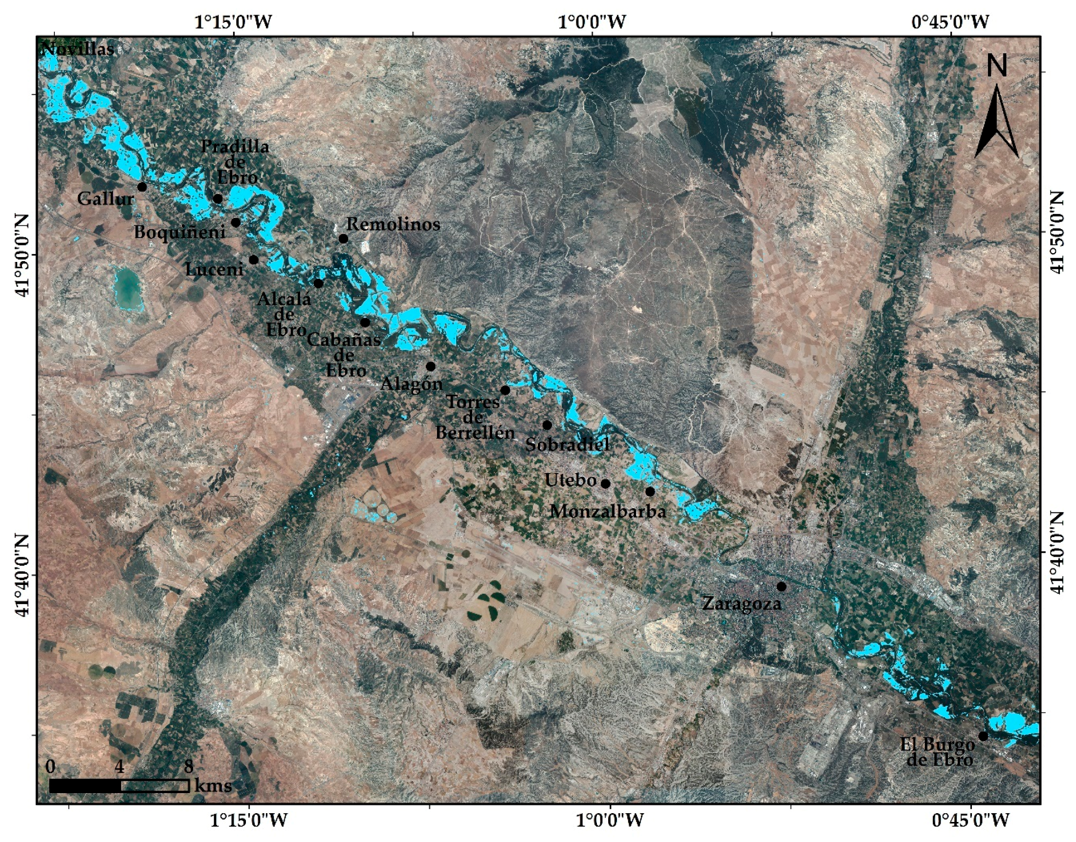
2. Study Area and Data Source
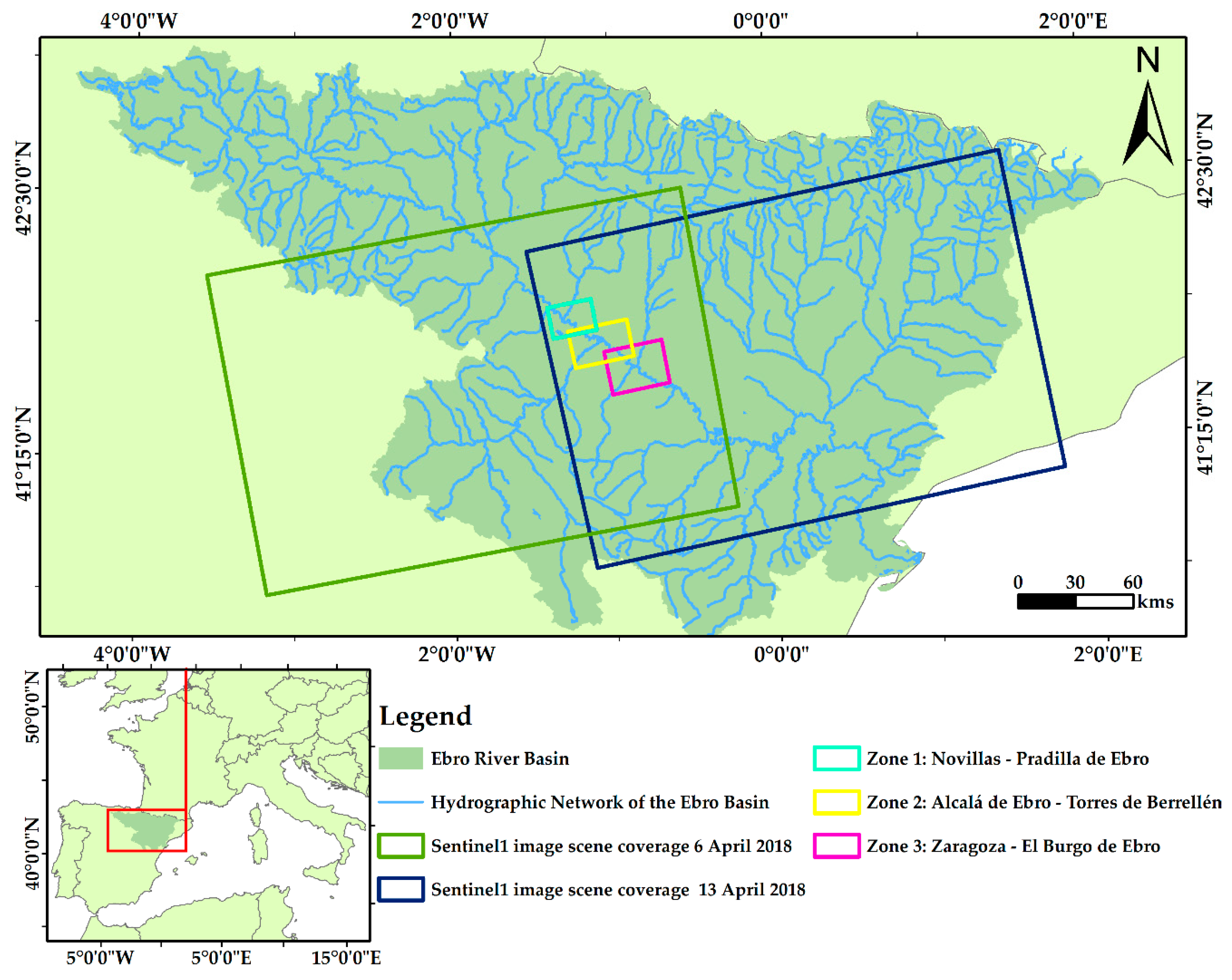
The Ebro river runs through seven autonomous communities and its hydrographic basin is one of the largest in the Iberian Peninsula. Its great extent favors geological, topographic, climatic, and water balance variability. The study area was focused in the middle basin of the Ebro, from the villages of Novillas to El Burgo de Ebro, and this entire section of the Zaragoza province (Figure 1). It is characterized by an average and very smooth slope; it has a high sinuous index with a meandering morphology and wide floodplains [18]. Irrigated fields, such as wheat, alfalfa, corn, barley, or rice, and permanent crops, such as vineyards, olive groves, or apple trees, are prevalent on the banks of the river [19].
The study of the great historical floods of the Ebro river, such as those that occurred in 1643, 1775, 1871, or 1961, and more recent ones, such as those of 2003 or 2015, provides information on the changing dynamics of the river’s course and how the Ebro has tried to consolidate in the flood zone, encountering man-made barriers to prevent the flooding from occurring [20]. The Ebro is one of the most regulated rivers in the Iberian Peninsula and suffers from frequent flooding [21]. The data supplied by the Hydrological Information Systems (SAIH, acronym in Spanish), in operation since the end of 1997 at the CHE, has facilitated the correct management of the reservoirs of the basin and has helped to control the floods since then. They provide, among other data, information on the levels and water flows in the main rivers and affluents, as well as the level of dammed water in the reservoirs, through sensors or stations located therein. Table 1 shows the maximum values in the last three large floods of the Ebro River in 2003, 2015, and 2018 with data provided by the gauging stations of Castejón and Zaragoza [22]. The floods of 2003 and 2015 left maximum flow values higher than those of 2018. This is due, in part, to the fact that after the flood of 2015, measures were taken to improve the safety of the populations closest to the channel, restore the riverbed, create new deviation channels, and construct new containment infrastructure [23].
The winter of 2018 was one of the rainiest since records were first kept. In late February and in March, there were considerable episodes of rain and snowfall, accompanied by wind, throughout the Iberian Peninsula. This produced a high accumulation of water in the Ebro River Basin, especially in the upper and middle sections, and snow at the headwaters of the rivers. This was aggravated by the fact that extreme values of soil moisture had been reached, saturating it and increasing the runoff. Days before the event, some reservoirs in the basin had been preventively drained. Between 7 and 12 April, an extraordinary flood, which is the object of study of this article, took place. This was due to persistent, widespread, and very significant rainfall, and also snowfall at heights between 800 and 1600 m, with lower temperatures that were unusual for this time of the year. To this was added, in the previous days, snow thawing in the Pyrenees in the early weeks of spring. In the first half of April, it rained in the basin more than three times the normal amount [24].
2.1. Hydraulic Parameters Characteristic of the Flood
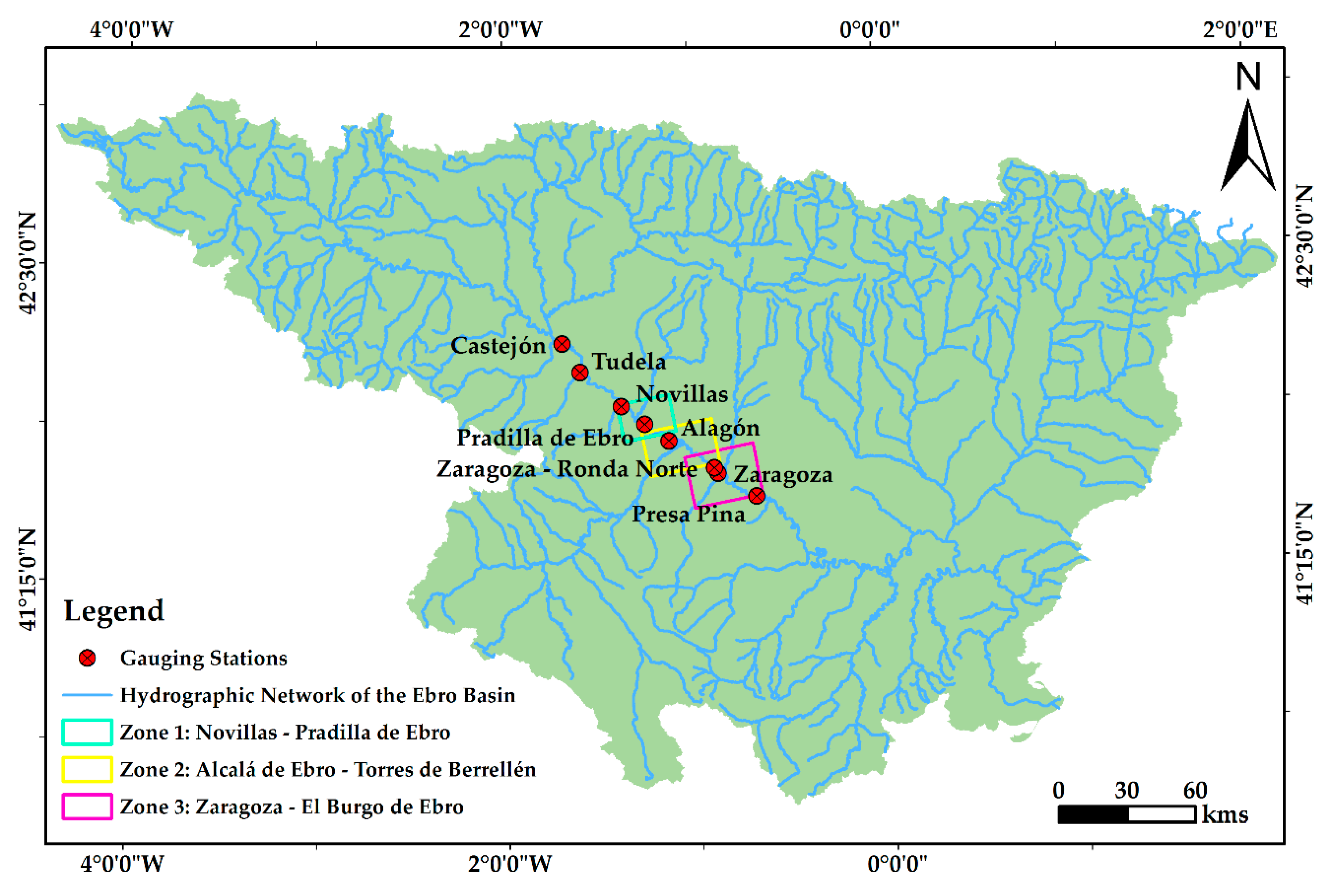
To know the maximum flow dates during the flood and to confirm the adequacy of the dates of the Sentinel-1 SAR images, data were taken from some of the gauging stations that exist along the course of the Ebro River (Figure 2). The values at the stations of Castejón and Tudela, in the province of Navarra and upstream of the study area, were taken into account, despite not being within the delimited study area. These give us an idea of the development of the flood and how the maximum flood points have been moving along down along the Ebro axis with time.
Table 2, representative of the year 2018, shows the values collected at the stations. This reflects the extraordinary flood of the Ebro in the month of April when it reached the highest values of the year. These data show the evolution of the flood from 13 to 15 April, obtaining the maximum annual level of accumulation in the Pina Dam, below the village of El Burgo de Ebro, on 15 April at 9:30 pm at 6.03 m, having had an average annual level of 4.48 m [22].
2.2. Sentinel-1 SAR Data
Synthetic Aperture RADAR (Radio Detection and Ranging) is a powerful active remote sensing technology used for several applications, including flood monitoring. RADAR are active systems that illuminate the Earth’s surface and therefore, images can be acquired by day during any lighting conditions, or at night, in the total absence of sunlight. In addition, these images are not affected by cloud cover, fog, or smoke because the RADAR signals have the ability to penetrate these covers [25,26].
Under the weather conditions in which floods occur, these types of images are the most suitable for study. Active radar systems incorporate an antenna that generates and transmits electromagnetic pulses (between 0.3 and 300 cm) to the Earth’s surface, and after interacting with the objects, the echoes of the backscattered signal are collected and amplified by a receiver at certain frequencies and polarization modes. Currently, there is a wide variety of SAR missions that have improved spatial resolution, bands, revisiting times, and polarization modes that have increased the monitoring potential [27].
The backscattering coefficient, or sigma nought (σ0), is the measure of the reflective strength of a radar target, defined as the per unit area on the ground, and is defined as the normalized measure of the radar return from a distributed target [28]. The amplitude and phase of the backscattered signal depends, among others, on the land surface properties, including the geometry, vegetation, roughness, and dielectric constant [29,30].
Continental waters, due to their low or null roughness in the absence of waves, behave like a specular surface, reflecting the radar return signal in a direction opposed to the sensor position, and therefore show very low backscatter values (negative) with respect to other land covers. This strong contrast in backscatter values allows the precise delimitation of flooded areas with SAR images. When a rough terrain has slopes with an angle that is more steep than the sensor depression angle, it generates shadow regions that appear without signal, very similar to the flooded areas, which can easily be confused. As flood areas tend to be flat, this effect is minor and is usually correctly delimited with detailed topographic information [31].
In this study, it is been used Sentinel-1 SAR images because of their features, configuration, and the free data set available online from Earth Observation (EO) data resources. Sentinel-1 SAR datasets, coming before and after the event, were downloaded via the Copernicus Open Access Hub platform [32]. The Sentinel-1 sensor is part of an ESA (European Space Agency) satellite constellation. It is composed of Sentinel-1A, launched on 3 April 2014, and Sentinel-1B, on 22 April 2016. Both satellites have a useful life of 7 years and a 12-day orbital repetition cycle (6 days between them). These temporal limitations of image capture mean that we did not have images of the day of the highest level of the Ebro at the study points. The available image that was closest to the moment of maximum flood was from 13 April 2018 and it was the one used for the development of the study.
Table 3 shows the characteristics of the two images used in the study. Usually, depending on the methodology used, the pre-event image serves as a reference and record of permanently flooded areas, while the post-event image serves to establish the differences with the initial image [33].
Each image has a coverage range of 250 km with a 5 × 20 m resolution. The images are Level-1 Ground Range Detected (GRD) products; this means that they were detected, multi-looked, and projected to the ground range using an Earth ellipsoid model [34]. The acquisition mode is Interferometric Wide Swath, and the images have a high resolution; the sensor pass is ascending, with incidence angles between 29° and 46°, and dual polarization, VV (Vertical-Vertical) and VH (Vertical-Horizontal). The study area is covered by VV and VH only according to the observation scenarios shown in Earth Observation Data Center for Water Resources Monitoring (EODC). In the free modes of IW (Interferometric Wide) Sentinel-1, only VV + VH polarization over land is available [35].
2.3. Additional Ebro Hydrographic Confederation Data
The Hydrological Planning Office of the CHE has been tracking air flights during flood episodes since the extraordinary flood that took place in February 2003. Flights are scheduled according to the time of the maximum flood peak as long as weather conditions allow it. Through these flights, oblique and vertical aerial photographs, as well as videos, are obtained, all in high resolution. This information provides the basis for the cartographic restitution of orthophotographs of the National Aerial Ortophotography Program (PNOA, acronym in Spanish) included in the General Spanish National Plan for Territory Observation (PNOT, acronym in Spanish) and to obtain, by digitization, the flood areas corresponding to each flood. This favors a greater understanding of the water behavior of the Ebro river over time.
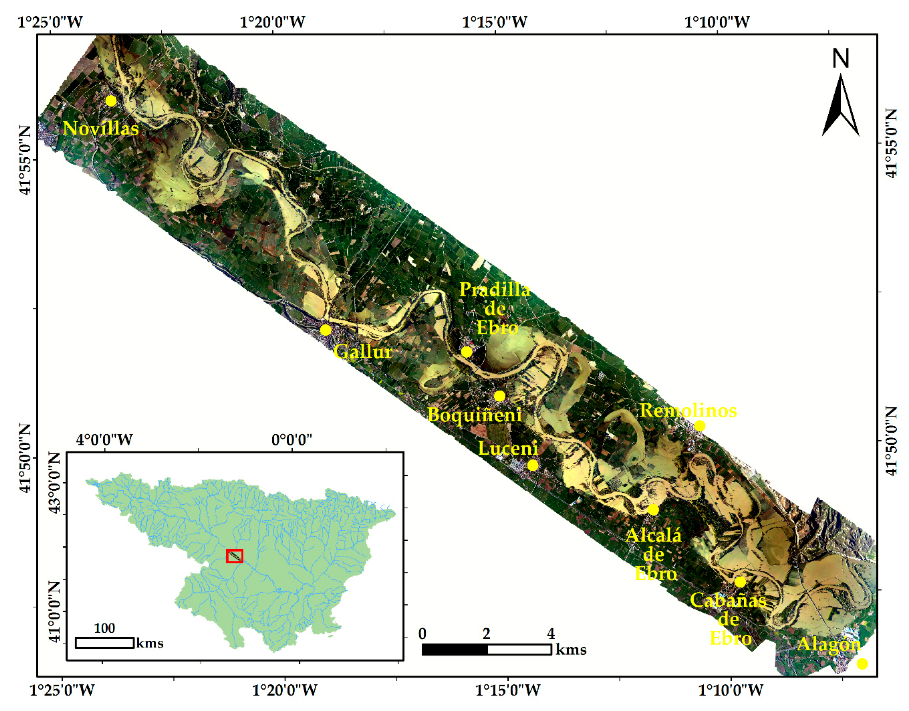
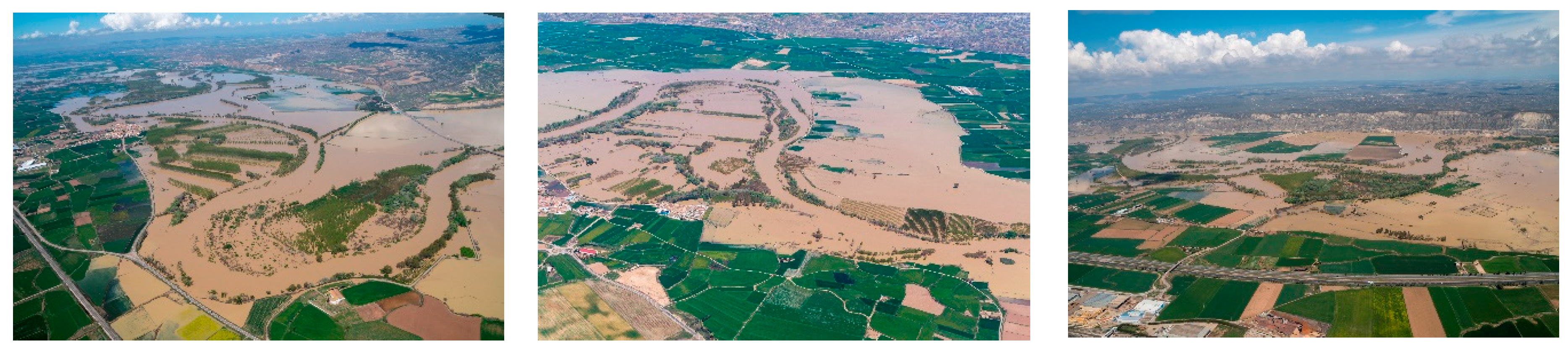
For the study area, a vertical aerial photograph corresponding to a part of the section that the CHE called “Ribera Alta” was used (Figure 3). It covers a region that goes from the village of Novillas to Alagón and was captured on 14 April 2018.
3. Procedures and Methodologies
3.1. SAR Sentinel-1 Data Pre-Processing
The images were processed with the free software SNAP (Sentinel Application Platform) Tool version 6.0.0. [37], created specifically by ESA for the analysis of the data captured by Sentinel satellites. It is a very powerful program that has the right tools, Sentinel Toolboxes, to perform an accurate and thorough treatment of the images and subsequently run the analysis. In Figure 4, the sequence of the steps followed for the pre-treatment of the images is shown.
In order to give continuity to the study, contribute to correct manipulation of images, and reduce the processing time, three subdivisions were made in each image, resulting in three areas of interest named after the most important towns and villages. These were zone 1—Novillas–Pradilla de Ebro, zone 2—Alcalá de Ebro–Torres de Berrellén, and zone 3—Zaragoza–El Burgo de Ebro (Figure 1).
The application of the right orbit helps to make the orbital data more accurate, improving geocoding and the subsequent processing results. With radiometric calibration, the value representing the radar backscatter intensity, in units of decibels, is taken for each pixel, and σ0-bands are generated for the two polarizations that we provide, VH and VV [38,39]. There is the possibility of obtaining other bands, but the σ0-band is the one that provides the best separation between terrestrial soil areas and those with water [40].
Permanent water bodies have temporal heterogeneity regarding backscattering [41]. The backscatter intensity values are usually below −20 dB and manifest themselves in dark, practically black tones. Applying the theoretical knowledge characteristic of the flat areas, the wave beams emitted by the sensor are reflected on the surface, which acts as a mirror, causing almost no return of energy towards the sensor; hence, its intensity value and representation in the radar image. There are surfaces that, at the scale of the measuring wavelength, behave as smooth and share almost identical scattering properties with water surfaces that can create “false positives” [42].
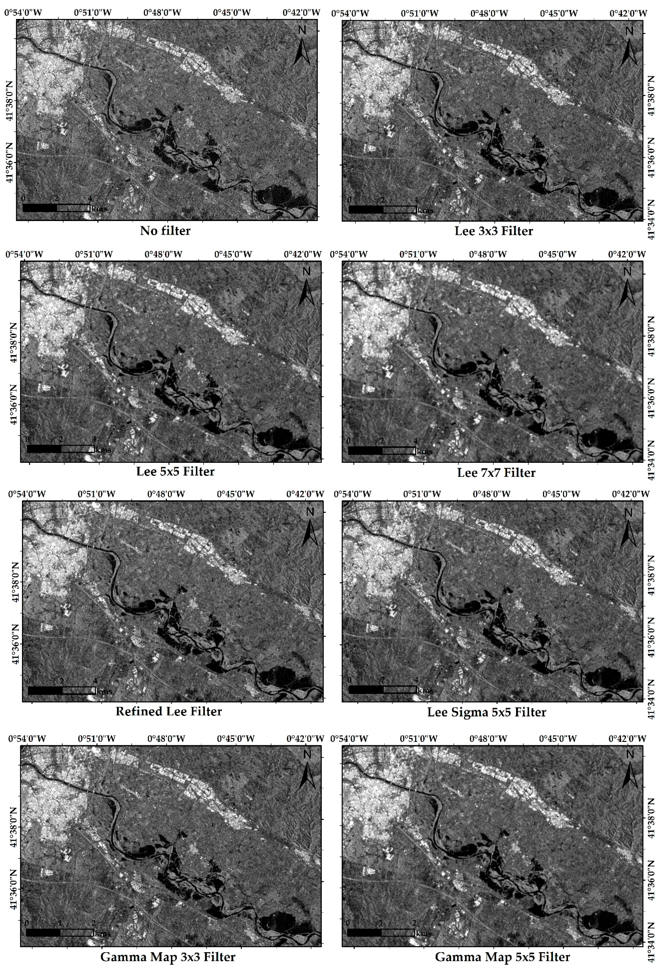
Speckle is represented in the images as mottled or granular noise. This causes degradation of the image quality and hinders its interpretation [43]. Mainly, noise is due to random oscillations of the signal returned to the sensor due to the interaction of the emitted wave with the rough terrain surfaces. There is no fixed procedure to suppress the speckle of RADAR images in flood extent mapping. The characteristics and configuration of each RADAR system, together with the conditions of the acquisition and characteristics of the land, establish the type and sequence of filters to be applied. The SNAP program has numerous filters, all of a statistical nature, to reduce this problem. A visual comparison was made with the filters Gamma Map, Lee, Refined Lee, and Lee Sigma, with different window sizes (Figure 5) in a small area, within the study area, which brings together flood areas, urban areas, and crop areas where the texture variability produced by the application of the different filters can be appreciated. The speckle filtering application does not modify the spatial detail and it is mostly used to achieve smoothing of the limits of the different forms represented, avoiding the loss of image details. The Gamma Map filter is based on the Bayes statistical analysis of the image and it works best for extensive areas, such as oceans, forests, or extensive fields [44]. The Lee filter uses statistical parameters, such as the mean and standard deviation, with a predetermined window size assessing different factors for smoothing. In homogeneous regions, such as flooded areas, the final pixel value is the linear average of neighboring pixels [45]. The Refined Lee filter provides a smoother texture in the image, minimizing radiometric and textural loss in the images [46,47]. The Lee Sigma filter uses a statistical distribution of the digital levels of a given area window chosen by the operator and estimates what pixel should be considered [48]. Taking into account mainly the topography, the geometry of the urban areas, the polarization, and the need to delimit those areas with smaller intensity values, the Lee filter with a window size 7 × 7 (m) was chosen as being most appropriate for the study.
The last common step in the pre-treatment of images is to perform a correction of the terrain and orthorectification. This mainly eliminates distortions due to changes in the topography and the angle of incidence with the ground with respect to the nadir. The geometric calibration used in this study was range doppler terrain correction and the digital elevation model (DEM)–SRTM-3Sec.
3.2. SAR Sentinel-1 Data Processing
Many authors have used various algorithms for the detection of non-permanent water surfaces. Among these approaches, we can highlight the supervised classification [49], automatic non-supervised classification [46,50], RGB combination [38,51], or the detection or calibration threshold technique [41,52,53,54,55,56,57]. In this study, the methodologies used were RGB composition and the calibrated thresholds technique. Before the application of any techniques and to perform a multitemporal analysis, it is necessary to unify in a single file the different bands of σ0 of the images before and after the event using a stack.
The RGB composition is an appropriate method to visualize multi-temporal modifications and facilitates the detection of changes on the terrain surface through a temporal color image [58]. It is a method based on the differences between the pre- and post-event images, and in which a combination of bands is set for these differences to become visually remarkable. These differences are defined by the change in the intensity value for the same pixel on different dates. The result is a multitemporal image to which a band is assigned to each of the primary colors to form an image of RGB composition [38].
The other methodology used was the calibration threshold technique, also called binarization. It is a simple and quick process that differentiates flooded areas from those that are not by generating histograms. The use of this methodology is not recommended for fast flash flooding, where mapping is urgently needed, and the presence of noise causes some uncertainty [59]. Knowing that the backscatter values in permanent waters and in flooded areas are generally the most negative and differ markedly from the following radiometric values caused by other physical changes, such as, for example, the moisture content of the soil, it is possible to establish any limit [40]. It is necessary to emphasize that an equitable distribution of water and land is necessary so that the histogram has two clear distributions to more precisely limit the threshold. Through the characteristic polarization histogram, we obtained the number of pixels in the image for certain values of intensity or backscatter. In this way, the threshold could be set manually between flooded areas and those that were not. Later, using a mathematical equation of bands, a new bi-colour image separating both zones was achieved [54].
4. Results and Discussion
4.1. RGB Composition Results
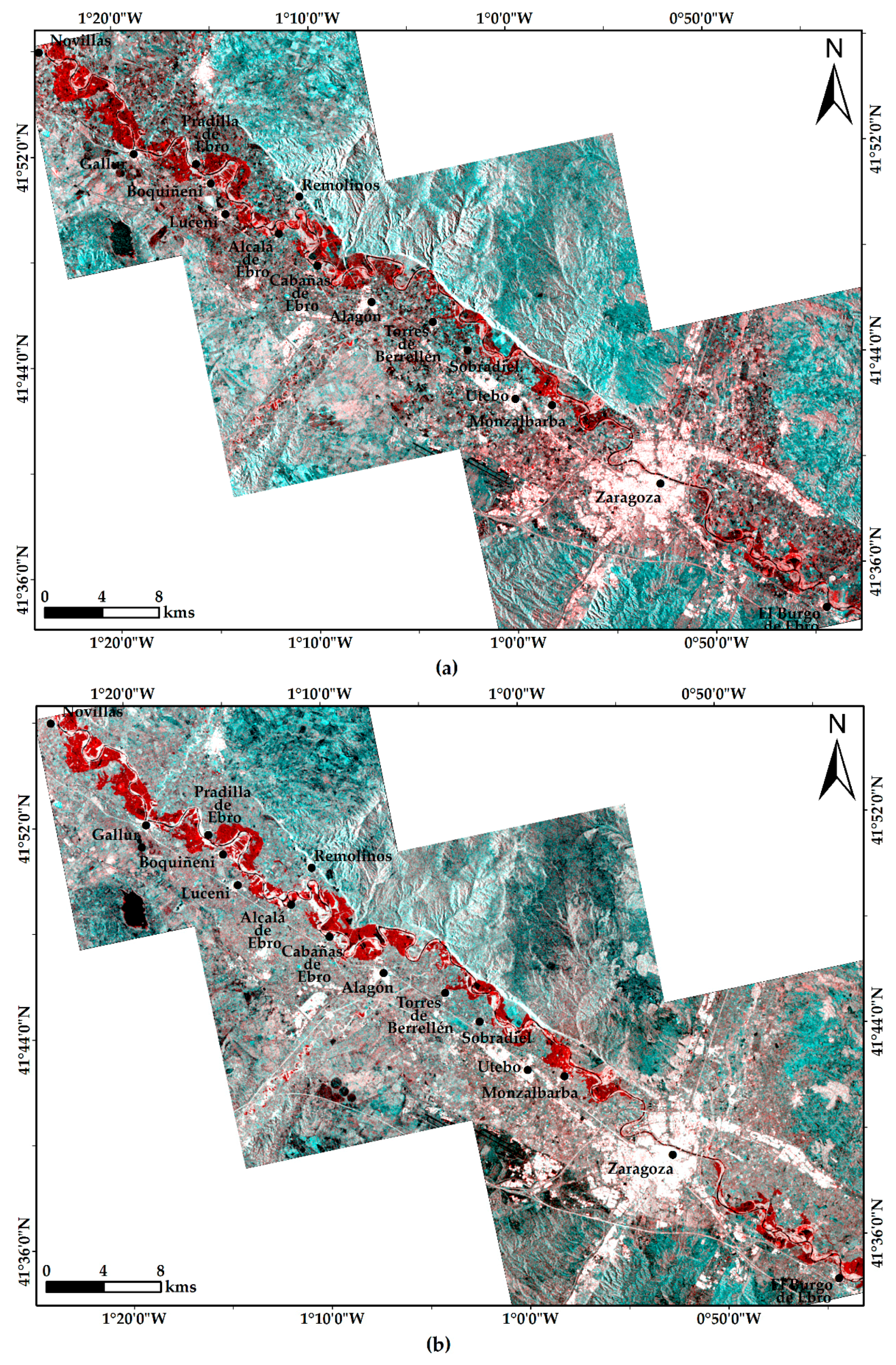
The combination of bands used for the application of the method was the image before the event for the R-band and the image after the event for the G- and B-band. Different results were obtained for the two polarizations, VV and VH, as can be seen in Figure 6. There are many possible combinations, but the chosen combination favors the visualization of the flooded areas. Water surfaces that are stable on both dates, such as the Ebro river or reservoirs, are represented in black. The populations, urban and industrial areas with very high intensity values, are observed in white. Those areas, with intermediate intensity values and in which there have been hardly any variations, are consolidated in blue tones. The light pink tones are characteristic of areas with high humidity while the red ones represent the flood surfaces in which the water has completely flooded.
It should be noted that right on the riverbank, the presence of massive riparian vegetation and vertical growth generates a double rebound dispersion or a volume dispersion (Figure 7). The vegetation structure and submerged status are conditioning factors of different scattering mechanisms that can happen, and therefore a range of backscatter values [60]. This, combined with the fact that the sensor used works in the C-band, with a penetration range in bare soil or vegetation that has a maximum of 5 cm, results in the presence of water not being shown even though the area was flooded. These areas are seen in white or slightly pink tones. For these areas, the use of an L-band sensor (23.5 cm) would provide greater penetration because the wavelength is longer than the size of the leaves within the tree mass [61]. In fully submerged locations, scattering dampening occurs as in an open flood, while scattering enhancement is observed in partially or unsubmerged locations because of the dihedral scattering dominates.
A correct choice of polarization optimizes the discrimination of flooded areas [33]. The results obtained in our polarization configurations and the contributions of [41,62] in the comparative studies of polarizations to monitor flood areas reaffirm that the VH polarization is more suitable for delimiting flooded areas. It generates well-defined and correctly defined surfaces, results that VV polarization cannot offer. VV polarization is clearly influenced by the roughness and heterogeneity of the terrain [33,63]. We can see this fact in the floodplains, where the roughness of the soil of the crops fields becomes more evident in the VV polarization.
4.2. Calibration Threshold Technique Results
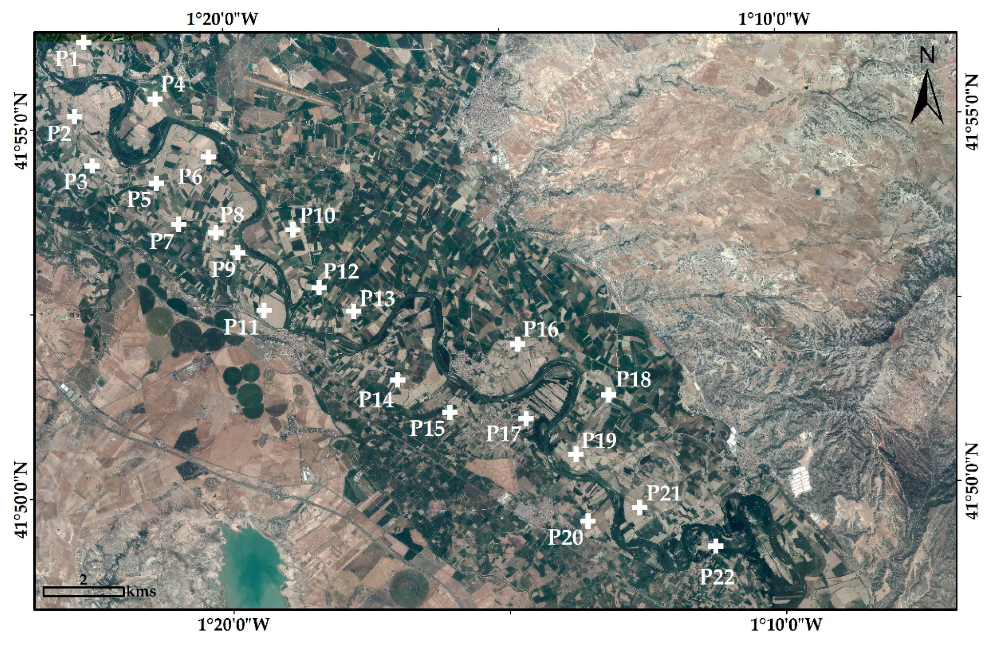
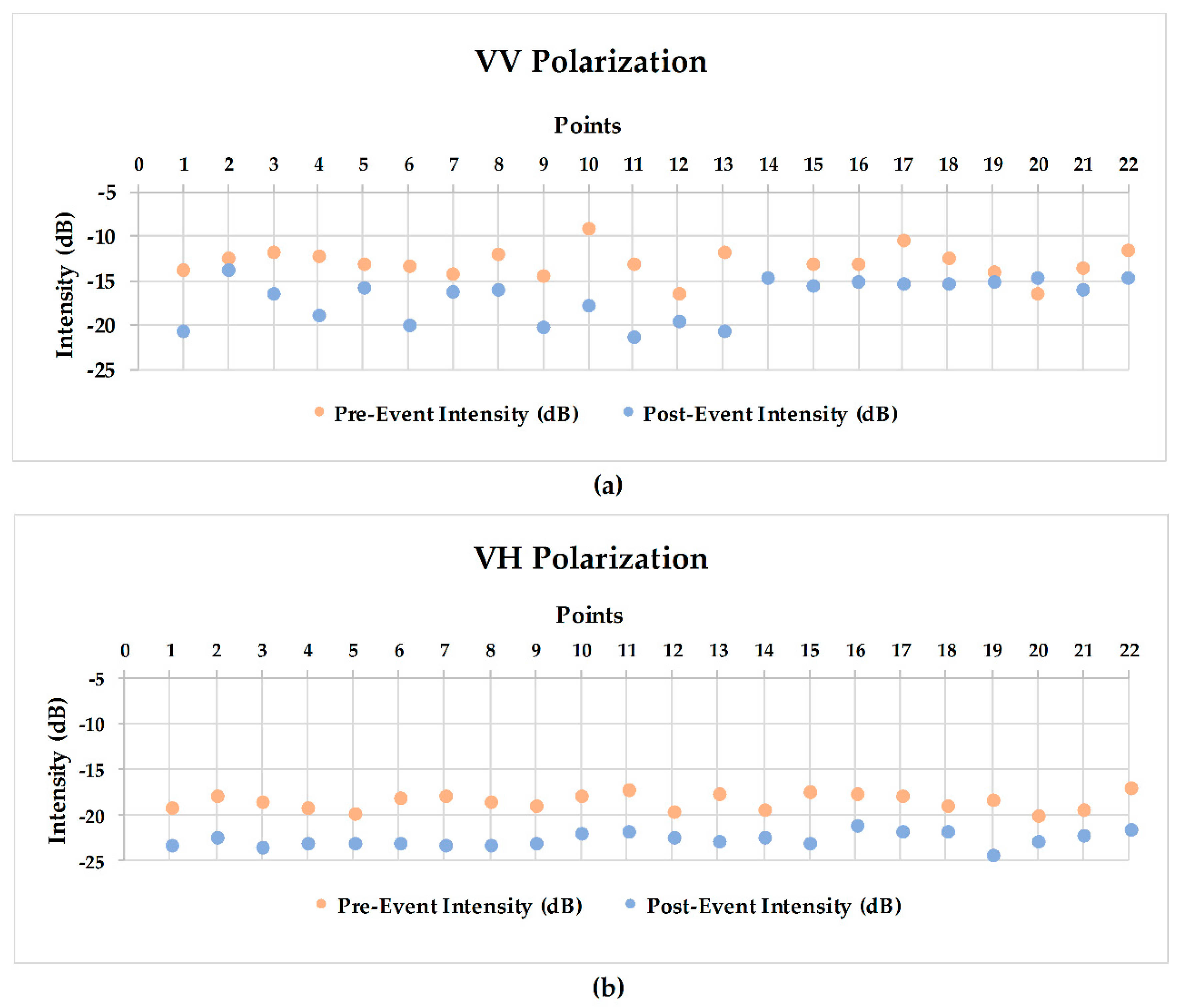
Before the application of this methodology for the extraction of several points from the radar images, specifically in zone 1 with VV and VH polarization, a comparison of how backscatter intensity values are modified in areas that have been flooded was considered (Figure 8). While the magnitude of intensity for the VV polarization, for both moments, is very variable and has a wide spectrum of values, the VH polarization is more defined within a certain range (Figure 9). The areas adjacent to the course of the river, mainly dedicated to cultivation, are characterized by partially rough surfaces and moderate vegetation. These move in values between −17 and −19 dB for the VH polarization, and between −11 and −15 dB for the VV polarization, with specific values that are out of this range. These same areas, subsequently flooded, reflect values between −21 and −24 dB approximately for VH polarization, and for VV, a wider range between −15 and −21 dB. The smooth surface generated by the sheet of water causes the backscatter intensity to decrease towards even more negative values.
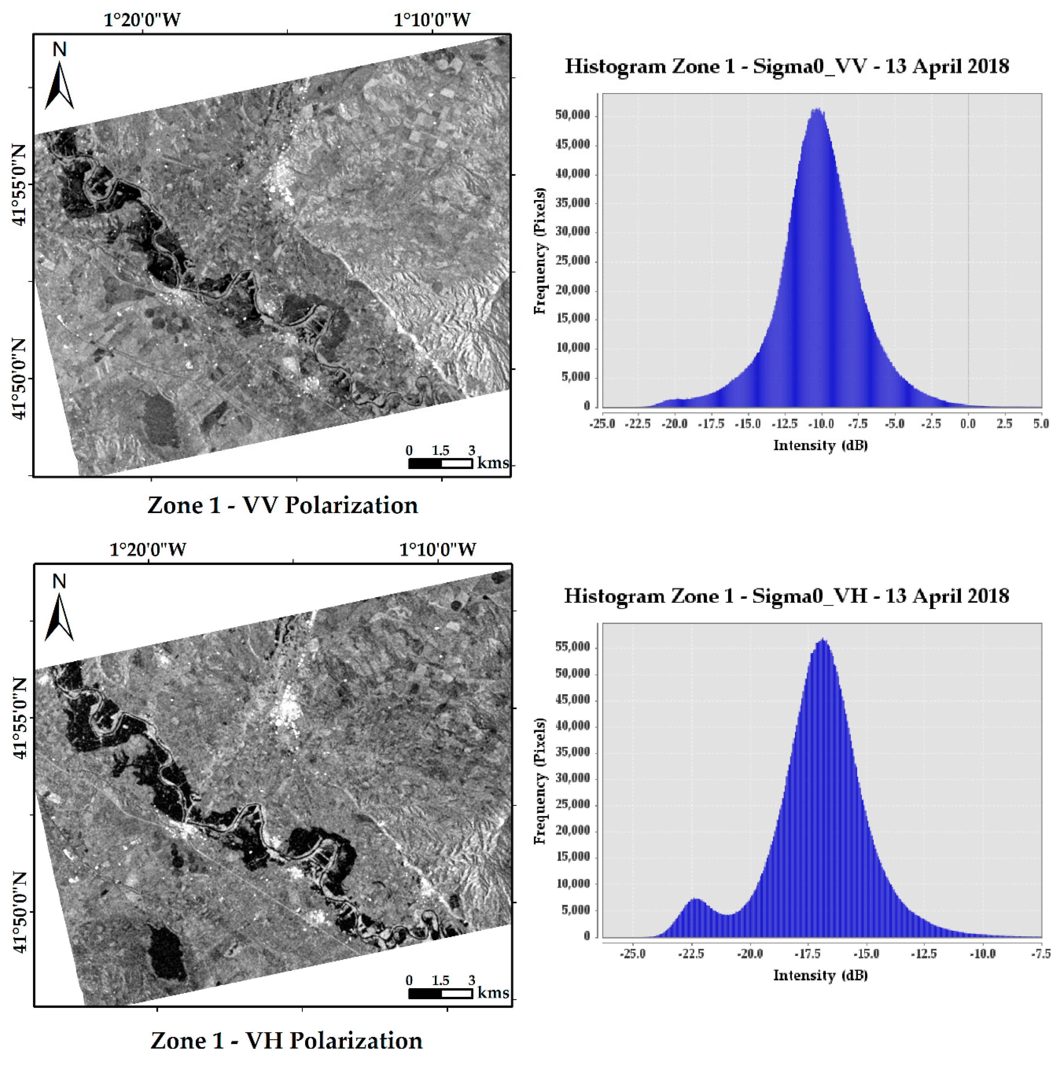
Through the graphics obtained by representation of characteristic points, we obtained an idea of the behavior of the radar on different surfaces. The calibration threshold methodology separated the dry zones from areas with the presence of a water sheet through the interpretation of histograms. In Figure 10, the relationship between polarizations and characteristic histograms for each of them is observed for the zone 1: Novillas–Pradilla de Ebro. The histogram of the VV polarization shows a very large curve representative of the intensity values ranging between −1.0 and −22 dB, a very wide spectrum characteristic of areas that range between very rough and moderately rough. While there is no clear projection of low backscatter values, the histogram of the VH polarization itself shows two clear populations where the specific intensity values of the image oscillate. This was chosen for further analysis. On the one hand, there is the curve that provides a greater number of pixels and that represents the areas without water, and on the other hand, a curve of smaller size and with smaller intensity values that represents the areas with water is shown. It is between both areas that the calibration limit can be set. Analyzing the histograms in greater depth, we observe that the cross polarization provides a wider range of backscatter values on surfaces with vegetation than the simple polarization, VV, which results in the latter omitting flooded areas [64].
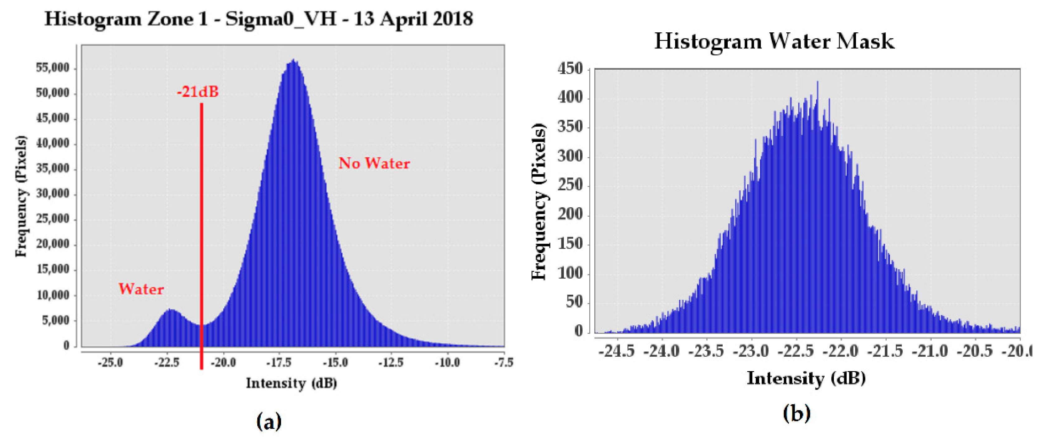
To further specify the boundary point between the areas with water and without water, a water mask was generated on the VH polarization image. This layer was created by randomly capturing some flooded areas within zone 1 and subsequently generating a histogram. In this way, intensity values were obtained in which only areas with water or flooded areas are shown, independent of the frequency or number of pixels taken. It should be noted that this layer serves only to confirm and verify the suitability of the threshold taken with the total histogram of the zone. The comparison of the histogram of the water mask obtained and the polarization VH histogram is shown in Figure 11. A significant spatial linear correlation between both histograms is shown, something that does not happen with VV polarization [56]. After studying the results, we conclude that the most representative values of the presence of the water range mostly between −21 and −24 dB, so −21 dB was considered. The threshold taken was therefore set to −21 dB.
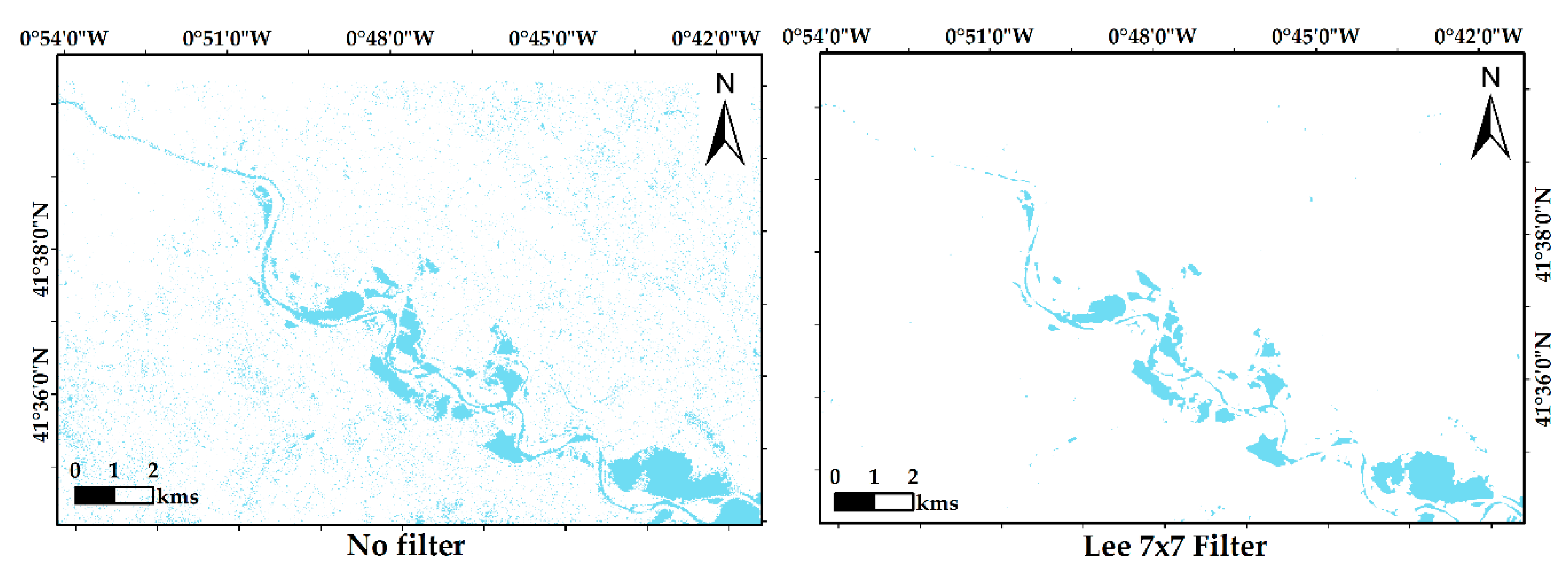
With the Raster-Band Maths tool of the SNAP program, a binary layer was generated in which, on the one hand, below −21 dB values are represented, representative of the water and flooded areas, and on the other, those above it that would show the dry zones. Figure 12 shows the areas with the presence of water that are observed in part of the study area for a radar image in which no filter was used and another for which the process of Lee 7 × 7 filtering was used. The unfiltered image has a large number of random pixels distributed by the image that give "false positives". All of them are points outside the flood area and the course of the river that have backscatter intensity values below −21 dB. On the other hand, the use of a filter minimizes this effect, favoring less overrepresentation errors.
The indicative layers of water presence, for the same specific area, were also generated for the other filters and different window sizes that were considered in the study (Refined Lee, Lee Sigma, and Gamma Map) and through which numerical data of the surfaces that show the presence of a water sheet were extracted (Table 4). It is quite significant that the use of one filter or another provides notable variations in the areas represented as water. Obviously, the unfiltered image is the one that generates more surface compared to any of the others that were filtered.
It is quite significant that the use of one filter or another provides notable variations in the areas represented as water. Obviously, the unfiltered image is the one that generates more surface compared to any of the others that were filtered. In comparison, the unfiltered image could provide even more than twice the area flooded than, for example, the image filtered with Lee 7 × 7. Therefore, the application of filtering is necessary not only for speckle reduction but to avoid errors when making quantitative calculations with images. The choice of the Lee 7 × 7 filter, which generates the least area, minimizes the presence of individual pixels outside the flood area and thus prevents overrepresentation in these areas.
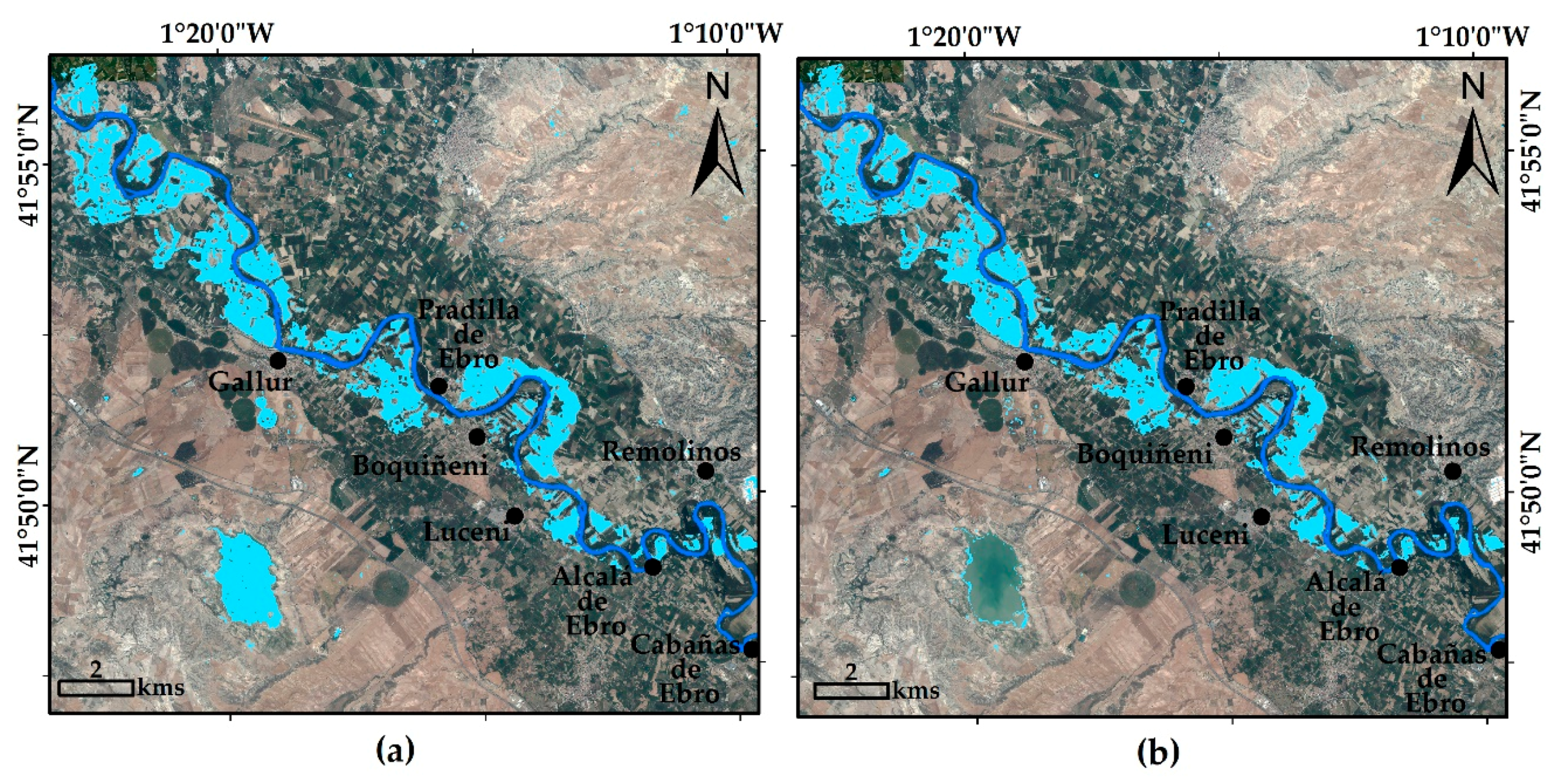
The choice of the Lee 7 × 7 filter was verified as being the most appropriate for the results of the present study. The process represented on the PNOA results in the map of zone 1 is shown in Figure 13. It should be taken into account that factors such as the characteristics of the terrain or the angle of incidence, can produce areas of shadow (see this effect in Figure 13a in the upper right where there is a mountainous area with higher topography). These have backscatter values similar to those with surfaces with the presence of water, causing overrepresentation of flooded areas [64]. Therefore, in order to avoid delimitation errors, the threshold technique could be combined with photointerpretation to add areas not identified by default or eliminate areas identified in excess, thus improving the quality of the results obtained [47]. It should also be considered that this technique does not discriminate between bodies of surface water (lakes, lagoons, reservoirs, wetlands) flooded areas. In order to eliminate this overrepresentation, a layer of only permanent areas was generated. This was created from the RADAR image of 6 April 2018, in which the avenue period had not yet begun. By subtracting the flood layer on 13 April 2018 and the one generated on day 6, with the Band Maths tool, we obtained a display of the temporary flood areas that are represented in Figure 13b.
Following the same steps for the other two zones gave the total flood map for the calibration threshold technique, as represented in Figure 14.
This technique applied to dual polarization images, VH in our case, gives good results in the extraction of water bodies, although these are small, but it has a number of limitations. These include, among other things, background noise. The calibration threshold is dependent on the characteristics of the surface to be captured and also on the specific parameters of the capture [65]. This implies that the threshold is not always fixed and cannot be generalized; it will have to be calculated in each study area.
4.3. Photointerpretation with Orthophoto Results
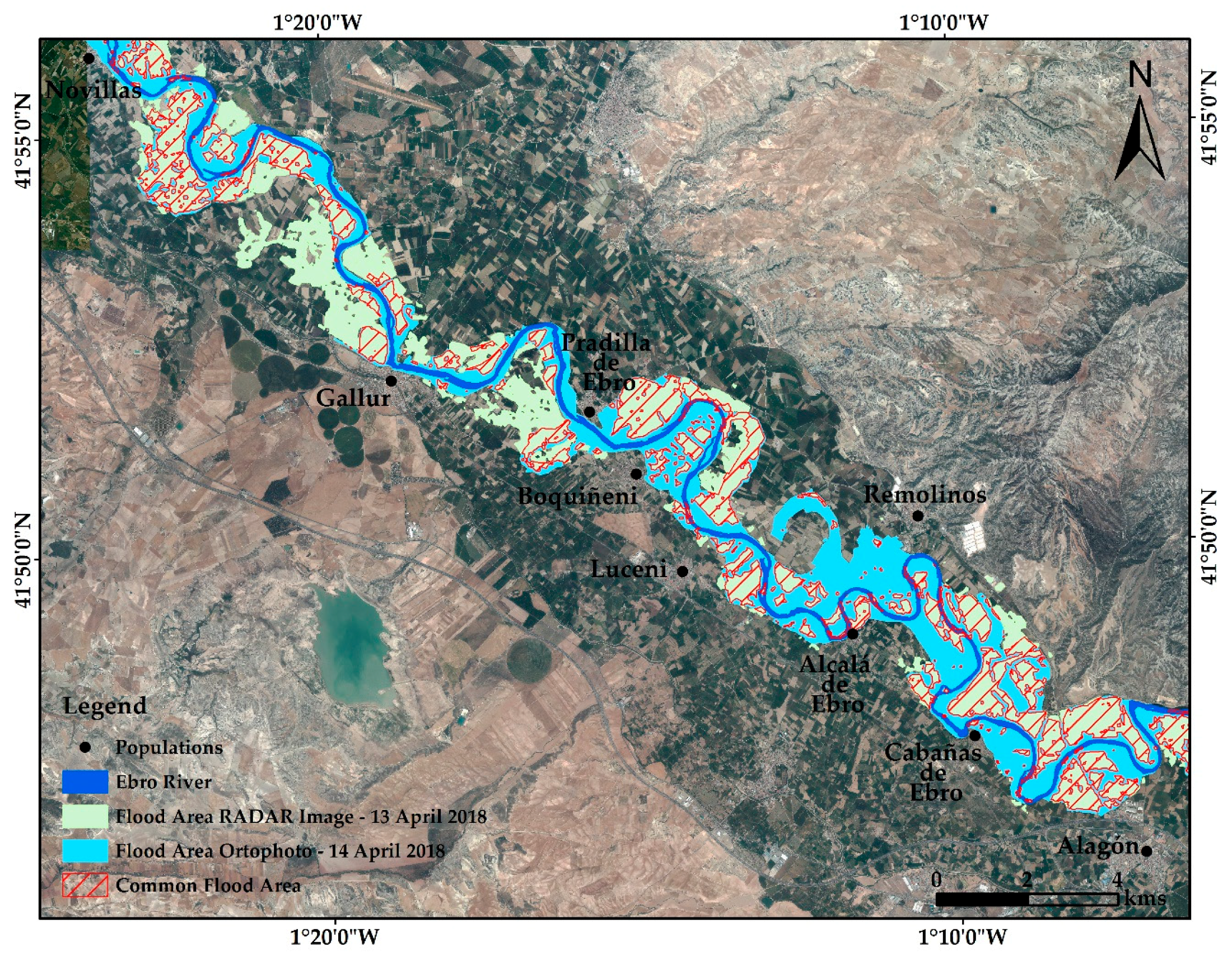
By analyzing the historical data of flows and levels in 2018, we can identify when the maximum annual flows of the Ebro were reached in the area of study. Specifically, they were reached in Novillas on 14 and 15 April at the Pina dam located downstream of the town of El Burgo de Ebro. In the villages between these two points, the maximum flow of the flood occurs between these two dates, migrating according to the direction of the river flow. In view of the data, it can be interpreted that the maximum flood day for the Ribera Alta was 14 April and that a comparison is possible between the RADAR image of 13 April and the orthophotography of the Ribera Alta. A comparison to determine both the flood areas was calculated through the result of the calibration threshold methodology and through photo interpretation of the flooded areas, and also calculation of the flooded surface for a specific day. Therefore, the areas in which the presence of water was perceived as flooding the fields were digitized, generating a vector layer on the orthophotography of the Ribera Alta. At the same time, the Ebro river was also digitized using the PNOA as a base map. For that purpose, the ArcGIS version 10.5 program was used to create the shape layers of the flood area and the Ebro river. In this way, the permanent river channel areas were discriminated from the temporarily inundated areas.
The flood areas of the RADAR image and the orthophotography are combined in Figure 15. In this way, common flood areas were obtained.
To establish the subsequent comparison, both layers were evaluated to calculate the flooded area overlapping the extent of flood areas mapped from both data sources (Table 5).
It should be noted that in the RADAR image, the maximum flood areas are located in the upper part of that section of the river, and that in the orthophotography, the maximum flood is in the lower part of the same study area. Considering flood mapping obtained from Sentinel-1 on 13 April 2018, and that flood mapping obtained from ortophotography one day after on 14 April 2018, the fast evolution of the flood areas is clear.
The variability in the value of the flood area is mainly due to the fact that the quality of the RADAR image, which needed numerous treatments, was reduced. This generates a loss of resolution quality that, together with the fact that there were intensity values that were not perceived as flooded areas (tree areas close to the riverbed, mainly), causes a reduction in the calculated area.
In October 2007, the European Directive 2007/60/CE was approved. This directive highlights the need to create flood mapping to delineate areas with greater exposure to these events and to generate hazard and flood risk maps. In accordance with the European Directive 2007/60/CE, Spain’s water governance system has made it possible to guarantee security and flood management.
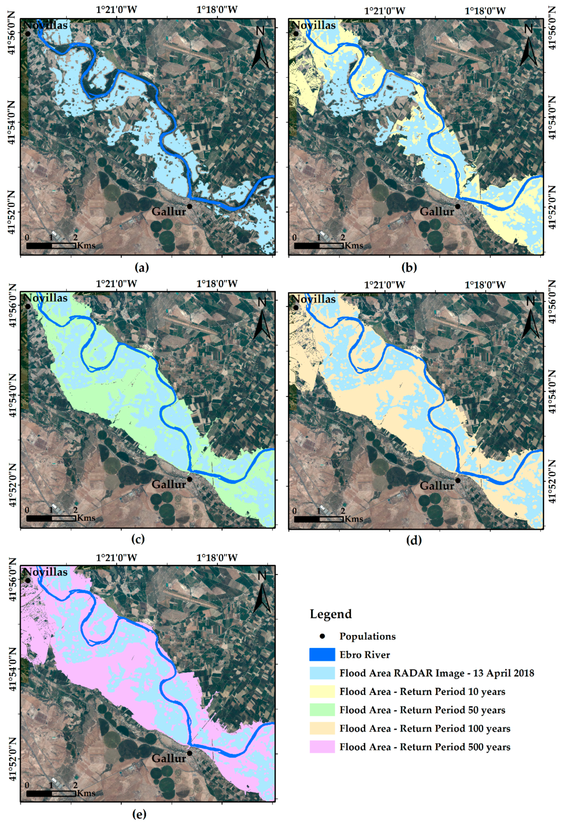
The Flood Risk Management Plans are based on the flood hazard maps (calculation of the flood zone) of the SNCZI for the 10, 50, 100, and 500 year return periods. SNCZI is the official public source for flood hazard information produced by MITECO [66].
The tools used by Spain’s government for the creation of the layers showing the flood return periods take into account the following: Hydrological studies that define the flows associated with the return periods considered in each moment; geomorphological studies, including a field cabinet analysis, LIDAR, or orthophotography images; historical studies; and a combination of the previous two and hydraulic studies, such as the generation of two-dimensional models [67]. However, they do not include SAR images as available base information to develop or validate the flood hazard maps.
In Figure 16, the result of the flooding map obtained with the RADAR image is compared with the layers with different return periods (10, 50, 100, 500 years) for a selected zone of the study area of SNCZI. On one hand, all flooded areas derived from Sentinel-1 SAR images are included inside the boundary for flood risk areas to 50, 100, and 500 years return period of SNCZI (Figure 16c–e. While, on the other hand, there are flooded areas that are outside the limits of the 10-year flood risk areas (Figure 16b). Therefore, we conclude that the results of flood area mapping derived from Sentinel-1 images are consistent with those of SNCZI, and correspond to a flood between 10 and 50 years of return. In view of the results obtained, the usefulness of Sentinel-1 images as baseline data for the improvement of the methodological guide is appreciated, and should be used as a new source of input, calibration, and validation for hydrological models to improve the accuracy of flood risk maps.
Flood maps obtained from Sentinel-1 SAR images complement and validate the information obtained by other means and help to understand the spatial and temporal evolution of the flood. Our results advise using flood maps derived from Sentinel-1 SAR images for the calibration and evaluation of hydrological models and as a data source that can complement and be compared with analysis obtained from other methodologies.
5. Conclusions
In this study, a functional methodology was proposed for flood monitoring at a necessary spatial resolution derived from SAR images. Specifically, it aimed to highlight the potential use of the Sentinel-1 SAR data sets of the European Earth Observation mission for flood monitoring occurring in the middle course of the Ebro River (Spain) in April 2018.
In SAR images, continental waters have strong contrast in the backscatter values due to their low or null roughness in the absence of waves, behaving like a specular surface that reflects the radar return signal in a direction opposed to the sensor position. However, they need a correction and filtering process (orbital parameters, radiometric, noise reduction speckle, and geometric geometric). Evaluating the different Sentinel-1 parameters, our analysis showed that the best results were obtained using VH polarization configuration. Concerning the need to apply numerous filters to reduce speckle, which also reduces the resolution quality of the images and has an effect on the final flood mapping, Lee filtering with a 7 × 7 window was the most appropriate option and it was proven that it favors the elimination of “false positives”.
Two methods were applied to detect and delimitate non-permanent water surfaces from Sentinel-1 SAR images. Method 1 RGB composition is based on differences between the pre- and post-event images, in which a combination of bands is set for identifying these differences as visually remarkable. The calibration threshold technique or binarization is based on a simple and quick process that differentiates flooded areas from those that are not from the characteristic polarization histogram using backscatter values in permanent waters and in flooded areas. The advantages of using the RGB composition methodology is that it guarantees clear differentiation between the areas of permanent flooding and the temporarily flooded ones, while achieving distinction through the technique of calibration thresholds requires other processes. Another advantage of the RGB methodology is that it detects the presence of massive riparian vegetation and vertical growth that can hide the presence of water, and it is essential to get a complete map of the flooded areas. In the calibration threshold technique, the most representative values of the presence of water were mainly between −21 and −24 dB; therefore, a central value of −21 dB was considered.
When comparing our flood maps with the flood areas digitalized from vertical aerial photographs planned by the Hydrological Planning Office of the Ebro Hydrographic Confederation, the results were consistent, even considering that the dates of both sources differed by a day. This confirmed and validated the use of Sentinel-1 SAR images to obtain flood maps with the required accuracy.
However, our flood maps derived from Sentinel-1 SAR images were consistent with flood risk areas provided by the SNCZI, and correspond to a flood between 10 and 50 years of return. In view of the results obtained, the usefulness of Sentinel-1 images as baseline data for the improvement of the methodological guide can be appreciated, and should be used as a new source of input, calibration, and validation for hydrological models to improve the accuracy of flood risk maps.
Finally, the development of methodologies that allow the synergy of different SAR missions (Sentinel-1, PAZ, Radarsat, TerraSAR-X, TanDEM-X, etc.) and multispectral optical systems will increase both the precision and the temporal resolution of flood monitoring, and should also be considered as powerful tools in the management and mitigation of the risks and defense against the adverse effects associated with floods.
Author Contributions
All authors have a significant contribution to final version of the paper. Conceptualization, F.C.C., and M.D.M.M.; Methodology, F.C.C., and M.D.M.M.; Supervision, F.C.C.; Processing SAR Sentinel-1 images, M.D.M.M.; Flood maps analysis, F.C.C., and M.D.M.M.; Investigation, F.C.C., and M.D.M.M.; Validation, F.C.C.; Writing—original draft, F.C.C., and M.D.M.M.; Writing—review and editing, F.C.C., and M.D.M.M.
Funding
This research received no external funding.
Acknowledgments
The authors would like to thank Hydrological Planning Office of the Ebro Hydrographic Confederation (Spanish Ministry for the Ecological Transition—MITECO) for data and photographs of the Ebro river flood reconnaissance aerial flights in April 2018, thank you to Cadonan for his diligent proofreading of this paper. Part of the present manuscript constituted the Master Thesis of the second of the authors, presented in the Master in Hydrology and Water Resources Management interuniversity of Alcalá University and Rey Juan Carlos University (Spain).
Conflicts of Interest
The authors declare no conflict of interest.
References
- Poff, N.L. Ecological response to and management of increased flooding caused by climate change. Philos. Trans. A Math. Phys. Eng. Sci. 2002, 360, 1497–1510. [Google Scholar] [CrossRef]
- The United Nations Office for Disaster Risk Reduction (UNISDR). The Human Cost of Weather Related Studies. 2015. Available online: https://www.unisdr.org/2015/docs/climatechange/COP21_Weather DisastersReport_2015_FINAL.pdf (accessed on 5 April 2019).
- European Environment Agency. Flood Risks and Environmental Vulnerability; Exploring the Synergies between Floodplain Restoration, Water Policies and Thematic Policies; European Environment Agency: Copenhagen, Danmark, 2016; pp. 9–15. [Google Scholar]
- Consorcio de compensación de seguros. Guía Para la Reducción de la Vulnerabilidad de los Edificios Frente a las Inundaciones. 2017. Available online: https://www.consorseguros.es/web/documents/10184/48069/ guia_inundaciones_completa_22jun.pdf (accessed on 17 September 2018).
- National Research Council. Hydrologic Hazards Science at the U.S. Geological Survey; The National Academies Press: Washington, DC, USA, 1999. [Google Scholar]
- Merz, B.; Aerts, J.; Arnbjerg-Nielsen, K.; Baldi, M.; Becker, A.; Bichet, A.; Blöschl, G.; Bouwer, L.M.; Brauer, A.; Cioffi, F.; et al. Floods and climate: Emerging perspectives for flood risk assessment and management. Nat. Hazards Earth Syst. Sci. 2014, 14, 1921–1942. [Google Scholar] [CrossRef]
- European Commission. Communication from the Commission to the European Parliament, the Council, the European Economic and Social Committee and the Committee of the Regions—An EU Strategy on Adaptation to Climate Change. 2013. Available online: https://ec.europa.eu/transparency/regdoc/rep/1/2013/EN/1-2013-216-EN-F1-1.pdf (accessed on 17 May 2018).
- Bioresita, F.; Puissant, A.; Stumpf, A.; Malet, J.F. Fusion of Sentinel-1 and Sentinel-2 image time series for permanent and temporary surface water mapping. Int. J. Remote Sens. 2019, 40, 9026–9049. [Google Scholar] [CrossRef]
- McFeeters, S.K. The Use of the Normalized Difference Water Index (NDWI) in the Delineation of Open Water Features. Int. J. Remote Sens. 1996, 17, 1425–1432. [Google Scholar] [CrossRef]
- Ji, L.; Zhang, L.; Wylie, B. Analysis of Dynamic Thresholds for the Normalized Difference Water Index. Photogramm. Eng. Remote Sens. 2009, 75, 1307–1317. [Google Scholar] [CrossRef]
- Shen, X.; Wang, D.; Mao, K.; Anagnostou, E.; Hong, Y. Inundation Extent Mapping by Synthetic Aperture Radar: A Review. Remote Sens. 2019, 11, 879. [Google Scholar] [CrossRef]
- Tomer, S.T.; Al Bitar, A.; Sekhar, M.; Zribi, M.; Bandyopadhyay, S.; Sreelash, K.; Sharma, A.K.; Corgne, S.; Kerr, Y. Retrieval and Multi-scale Validation of Soil Moisture from Multi-temporal SAR Data in a Semi-Arid Tropical Region. Remote Sens. 2015, 7, 8128–8153. [Google Scholar] [CrossRef]
- Filion, R.; Bernier, M.; Paniconi, C.; Chokmani, K.; Melis, M.; Soddu, A.; Talazac, M.; Lafortune, F.-X. Remote sensing for mapping soil moisture and drainage potential in semi-arid regions: Applications to the Campidano plain of Sardinia, Italy. Sci. Total Environ. 2016, 573, 862–876. [Google Scholar] [CrossRef]
- Ulaby, F.T.; Moore, R.K.; Fung, A.K. Microwave Remote Sensing: Active and Passive, Volume 2, Radar Remote Sensing and Surface Scattering and Emission Theory; Addison-Wesley: Reading, MA, USA, 1983; pp. 1840–1852. [Google Scholar]
- Kelly, R.; Davie, T.; Atkinson, P. Explaining temporal and spatial variation in soil moisture in a bare field using SAR imagery. Int. J. Remote. Sens. 2003, 24, 3059–3074. [Google Scholar] [CrossRef]
- Smith, L. Satellite remote sensing of river inundation area, stage, and discharge: A review. Hydrol. Process. 1997, 11, 1427–1439. [Google Scholar] [CrossRef]
- European Exchange Circle on Flood Mapping (EXCIMAP). Handbook on Good Practices for Flood Mapping in Europe. Available online: https://ec.europa.eu/environment/water/flood_risk/flood_atlas/pdf/ handbook_goodpractice.pdf (accessed on 10 September 2019).
- Sánchez Fabre, M.; Ballarán Ferrer, D.; Mora, D.; Ollero, A.; Serrano-Notivoli, R.; Saz, M. Las Crecidas del Ebro Medio en el Comienzo del Siglo XXI; XXIV Congreso de la Asociación de Geógrafos Españoles. Análisis espacial y representación geográfica: Innovación y aplicación; Universidad de Zaragoza y Asociación de Geógrafos Españoles: Zaragoza, Spain, 2015; pp. 1853–1862. [Google Scholar]
- Confederación Hidrográfica del Ebro, CHE. Available online: http://www.chebro.es (accessed on 15 February 2019).
- Galván Plaza, R. Cuatro grandes inundaciones históricas del Ebro en la ciudad de Zaragoza: 1643, 1775, 1871 y 1961. Pap. De Geogr. 2018, 64, 7–25. [Google Scholar] [CrossRef]
- Pueyo Anchuela, Ó.; Revuelto, C.; Casas Sainz, A.; Rajamo Cordero, J.; Pocovi, A. Las crecidas del Ebro de febrero/marzo de 2015. ¿Qué hemos aprendido y qué falta por aprender? Geogaceta 2016, 60, 119–122. [Google Scholar]
- Sistema Automático de Información Hidrológica de la Cuenca Hidrográfica del Ebro (SAIH of the CHE). Available online: http://www.saihebro.com/saihebro/index.php (accessed on 12 March 2019).
- Polanco Fernández, L. Obras de restauración fluvial en el ámbito del Plan PIMA Adapta. In Proceedings of the Conference: La Gestión del Riesgo de Inundación Fluvial en el Contexto del Cambio Climático, Madrid, Spain, 10 December 2018. [Google Scholar]
- Rodríguez Marcos, F.J. Principales episodios de inundaciones de 2018. In Proceedings of the Conference: La Gestión del Riesgo de Inundación Fluvial en el Contexto del Cambio Climático, Madrid, Spain, 10 December 2018. [Google Scholar]
- Martínez, J.M.; Toan, T. Mapping of flood dynamics and vegetation spatial distribution in the Amazon floodplain using multitemporal SAR data. Remote Sens. Environ. 2007, 108, 209–223. [Google Scholar] [CrossRef]
- Cunjian, Y.; Yiming, W.; Siyuan, W.; Zengxiang, Z.; Shifeng, H. Extracting the flood extent from satellite SAR image with thesupport of topographic data. In Proceedings of the International Conferences on Info-Tech and Info-Net. Networks (ICII 2001), Beijing, China, 29 October–1 November 2001; IEEE: Piscataway, NJ, USA, 2001; Volume 1, pp. 87–92. [Google Scholar]
- Argenti, F.; Lapini, A.; Alparone, L. A tutorial on speckle reduction in synthetic aperture radar images, IEEE Geosci. Remote Sens. Mag. 2013, 1, 6–35. [Google Scholar]
- European Space Agency (ESA). The ASAR User Guide. Available online: https://earth.esa.int/handbooks/asar/toc.html (accessed on 10 July 2019).
- Gorrab, A.; Zribi, M.; Baghdadi, N.; Mougenot, B.; Fanise, P.; Chabaane, Z.L. Retrieval of both soil moisture and texture using TerraSAR-X images. Remote Sens. 2015, 7, 10098–10116. [Google Scholar] [CrossRef]
- Zribi, M.; Dechambre, M. A new empirical model to retrieve soil moisture and roughness from C-band radar data. Remote Sens. Environ. 2002, 84, 42–52. [Google Scholar] [CrossRef]
- Twele, A.; Cao, W.X.; Plank, S.; Martinis, S. Sentinel-1-based flood mapping: A fully automated processing chain. Int. J. Remote Sens. 2016, 37, 2990–3004. [Google Scholar] [CrossRef]
- European Space Agency (ESA). Copernicus Open Access Hub. Available online: https://scihub.copernicus.eu/dhus/#/home (accessed on 2 May 2019).
- Klemas, V. Remote sensing of floods and flood-prone areas: An overview. J. Coast. Res. 2015, 31, 1005–1013. [Google Scholar] [CrossRef]
- ESA Sentinel Online. User Guides and Technical Guides of Sentinel-1 SAR. Available online: https://sentinel.esa.int/web/sentinel (accessed on 8 August 2019).
- ESA Sentinel Online. Product Types and Processing Levels. Available online: https://sentinel.esa.int/web/ sentinel/user-guides/sentinel-1-sar/product-types-processing-levels (accessed on 8 August 2019).
- Confederación Hidrográfica del Ebro, CHE. Ministerio Para la Transición Ecológica; Gobierno de España. Vuelos aéreos de reconocimiento para la inundación del río Ebro en abril de 2018; CHE: Zaragoza, Spain, 2018. [Google Scholar]
- SNAP Software Version 6.0.0. Available online: https://step.esa.int/main/download/snap-download (accessed on 22 December 2018).
- Tavus, B.; Kocaman, S.; Gokceoglu, C.; Nefeslioglu, H.A. Considerations on the use of Sentinel-1 data in flood mapping in urban areas: Ankara (Turkey) 2018 floods. Int. Arch. Photogramm. Remote Sens. Spat. Inf. Sci. 2018, XLII-5, 575–581. [Google Scholar] [CrossRef]
- Ban, H.-J.; Kwon, Y.-J.; Shin, H.; Ryu, H.-S.; Hong, S. Flood monitoring using satellite-based RGB composite imagery and refractive index retrieval in visible and near-infrared bands. Remote Sens. 2017, 9, 313. [Google Scholar] [CrossRef]
- Bioresita, F.; Puissant, A.; Stumpf, A.; Malet, J.-P. A method for automatic and rapid mapping of water surfaces from Sentinel-1 imagery. Remote Sens. 2018, 10, 217. [Google Scholar] [CrossRef]
- Martinis, S.; Rieke, C. Backscatter analysis using multi-temporal and multi-frequency SAR data in the context of flood mapping at river Saale, Germany. Remote Sens. 2015, 7, 7732–7752. [Google Scholar] [CrossRef]
- Henry, J.-B.; Chastanet, P.; Fellah, K.; Desnos, Y.-L. Envisat multipolarized ASAR data for flood mapping. Int. J. Remote Sens. 2006, 27, 1921–1929. [Google Scholar] [CrossRef]
- Kudahetty, C. Flood Mapping Using Synthetic Aperture Radar in the Kelani Ganga and the Bolgoda Basins, Sri Lanka; Master of Science in Geo-information Science and Earth Observation; University of Twente: Enschede, The Netherlands, 2012. [Google Scholar]
- Senthilnath, J.; Handiru, V.; Rajendra, R.; Omkar, S.N.; Mani, V.; Diwakar, P. Integration of speckle de-noising and image segmentation using Synthetic Aperture Radar image for flood extent extraction. J. Earth Syst. Sci. 2013, 122, 559–572. [Google Scholar] [CrossRef]
- Park, J.-M.; Song, W.J.; Pearlman, W.A. Speckle filtering of SAR images based on adaptive windowing. IEE Proc. Vis. Image Signal Process. 1999, 146, 191–197. [Google Scholar] [CrossRef]
- Borah, S.B.; Sivasankar, T.; Ramya, M.N.S.; Raju, P.L.N. Flood inundation mapping and monitoring in Kaziranga National Park, Assam using Sentinel-1 SAR data. Environ. Monit. Assess. 2018, 190, 520. [Google Scholar] [CrossRef]
- Ezzine, A.; Darragi, F.; Rajhi, H.; Ghatassi, A. Evaluation of Sentinel-1 data for flood mapping in the upstream of Sidi Salem dam (Northern Tunisia). Arab. J. Geosci. 2018, 11, 170. [Google Scholar] [CrossRef]
- García, R.; González, C.; De la Vega, R.; Valverde, A.; Seben, E. Análisis del Comportamiento de Filtros de Reducción de Speckle en Imágenes ERS2-SAR; Teledetección y Desarrollo Regional; X Congreso de Teledetección: Cáceres, Spain, 2003; pp. 325–328. [Google Scholar]
- Chapman, B.; McDonald, K.; Shimada, M.; Rosenqvist, A.; Schroeder, R.; Hess, L. Mapping regional inundation with spaceborne L-Band SAR. Remote Sens. 2015, 7, 5440–5470. [Google Scholar] [CrossRef]
- Martinis, S.; Twele, A.; Voigt, S. Unsupervised extraction of flood-induced backscatter changes in SAR data using Markov image modeling on irregular graphs. IEEE Trans. Geosci. Remote Sens. 2011, 49, 251–263. [Google Scholar] [CrossRef]
- Perrou, T.; Garioud, A.; Parcharidis, I. Use of Sentinel-1 imagery for flood management reservoir-regulated river basin. Front. Earth Sci. 2018, 12, 506–520. [Google Scholar] [CrossRef]
- Cao, H.; Zhang, H.; Wang, C.; Zhang, B. Operational Flood Detection Using Sentinel-1 SAR Data over Large Areas. Water 2019, 11, 786. [Google Scholar] [CrossRef]
- Martinis, S.; Twele, A.; Voigt, S. Towards operational near real-time flood detection using a split-based automatic thresholding procedure on high resolution TerraSAR-X data. Nat. Hazards Earth Syst. Sci. 2009, 9, 303–314. [Google Scholar] [CrossRef]
- Psomiadis, E. Flash flood area mapping utilising Sentinel-1 radar data. In Proceedings of the SPIE 10005, Earth Resources and Environmental Remote Sensing/GIS Applications, Dresden, Germany, 11 November 2013; VII 100051G. SPIE: Edimburgh, UK, 2016. [Google Scholar]
- Dumitrascu, N.; Oniga, E.; Florian, S.; Marcu, C. Floods damage estimation using sentinel-1 satellite images. Case study: Galati County, Romania. RevCAD. J. Geod. Cadas. 2017, 22, 115–122. [Google Scholar]
- Pham-Duc, B.; Prigent, C.; Aires, F. Surface Water Monitoring within Cambodia and the Vietnamese Mekong Delta over a Year, with Sentinel-1 SAR Observations. Water 2017, 9, 366. [Google Scholar] [CrossRef] [Green Version]
- Zhang, B.; Wdowinski, S.; Oliver-Cabrera, T.; Koirala, R.; Jo, M.J.; Osmanoglu, B. Mapping the extent and magnitude of severe flooding induced by hurricane Irma with multi-temporal Sentinel-1 SAR and InSAR observations. Int. Arch. Photogramm. Remote Sens. Spat. Inf. Sci. 2018, XLII-3, 2237–2244. [Google Scholar] [CrossRef] [Green Version]
- Amitrano, D.; Guida, R.; Ruello, G. Multitemporal SAR RGB Processing for Sentinel-1 GRD Products: Methodology and Applications. IEEE J. Select. Top. Appl. Earth Obs. Remote Sens. 2019, 12, 1497–1507. [Google Scholar] [CrossRef]
- Westerhoff, R.S.; Kleuskens, M.P.H.; Winsemius, H.C.; Huizinga, H.J.; Brakenridge, G.R.; Bishop, C. Automated global water mapping based on wide-swath orbital synthetic-aperture radar. Hydrol. Earth Syst. Sci. 2013, 17, 651–663. [Google Scholar] [CrossRef] [Green Version]
- Shen, X.; Hong, Y.; Qin, Q.; Chen, S.; Grout, T. A backscattering enhanced canopy scattering model based on mimics. In Proceedings of the American Geophysical Union (AGU) 2010 Fall Meeting, San Francisco, CA, USA, 13–17 December 2010. [Google Scholar]
- Townsend, P.A. Relationships between forest structure and the detection of flood inundation in forested wetlands using C-band SAR. Int. J. Remote Sens. 2002, 23, 443–460. [Google Scholar] [CrossRef]
- Matgen, P.; Schumann, G.; Henry, J.-B.; Hoffmann, L.; Pfister, L. Integration of SAR-derived river inundation areas, high-precision topographic data and a river flow model toward near real-time flood management. Int. J. Appl. Earth Obs. Geoinf. 2007, 9, 247–263. [Google Scholar] [CrossRef]
- Manjusree, P.; Prasanna Kumar, L.; Bhatt, C.M.; Srinivasa Rao, G.; Bhanumurthy, V. Optimization of threshold ranges for rapid flood inundation mapping by evaluating backscatter profiles of high incidence angle SAR images. Int. J. Disaster Risk Sci. 2012, 3, 113–122. [Google Scholar] [CrossRef] [Green Version]
- Clement, M.; Kilsby, C.; Moore, P. Multi-temporal SAR flood mapping using change detection. J. Flood Risk Manag. 2017, 11, 152–168. [Google Scholar] [CrossRef]
- Nguyen, D. Automatic detection of surface water bodies from Sentinel-1 SAR images using Valley-Emphasis method. Vietnam Earth Sci. 2016, 37, 328–343. [Google Scholar]
- Ministerio para la Transición Ecológica, MITECO. 2017. Available online: https://www.miteco.gob.es/es/cartografia-y-sig/ide/descargas/agua/zi-lamina.aspx (accessed on 6 May 2019).
- Ministerio para la Transición Ecológica, MITECO. Guía Metodológica Para el Desarrollo del Sistema Nacional de Cartografía de Zonas Inundables, 1st ed.; Ministerio de Medio Ambiente y Medio Rural y Marino: Madrid, Spain, 2011; pp. 19–52.
Figure 1.
Location map and study areas.

Figure 2.
Location map of the gauging stations considered in the study.

Figure 3.
Ribera Alta orthophotography dated 14 April 2018. (Orthophotographs source: CHE, 2018 [36]).
Figure 3.
Ribera Alta orthophotography dated 14 April 2018. (Orthophotographs source: CHE, 2018 [36]).

Figure 4.
Flowchart showing the preprocessing chain used in RADAR SAR Sentinel-1 images.

Figure 5.
Detailed images of a section of zone 3 (Zaragoza–El Burgo de Ebro), 13 April 2018, after the flood event, with VH polarization in which the comparison is shown between the unfiltered image and the result of the application of different filters of different window sizes.
Figure 5.
Detailed images of a section of zone 3 (Zaragoza–El Burgo de Ebro), 13 April 2018, after the flood event, with VH polarization in which the comparison is shown between the unfiltered image and the result of the application of different filters of different window sizes.

Figure 6.
General flood map of the entire study area using RGB composition created from the RADAR images of 6 April 2018 and 13 April 2018: (a) in VV and (b) in VH polarization with a Lee 7 × 7 window size filter.
Figure 6.
General flood map of the entire study area using RGB composition created from the RADAR images of 6 April 2018 and 13 April 2018: (a) in VV and (b) in VH polarization with a Lee 7 × 7 window size filter.

Figure 7.
Aerial views of the study area on 14 April 2018, showing the flood of the Ebro and the characteristic riverbank vegetation as highly flooded (Source: CHE, 2018 [36]).
Figure 7.
Aerial views of the study area on 14 April 2018, showing the flood of the Ebro and the characteristic riverbank vegetation as highly flooded (Source: CHE, 2018 [36]).

Figure 8.
Location map of the points considered in the comparison of backscatter intensity before and after the flooding event.
Figure 8.
Location map of the points considered in the comparison of backscatter intensity before and after the flooding event.

Figure 9.
Graphical representation of the values of backscatter intensity before and after the event, for the VV (a) and VH (b) polarization, for the indicated points.
Figure 9.
Graphical representation of the values of backscatter intensity before and after the event, for the VV (a) and VH (b) polarization, for the indicated points.

Figure 10.
Representation of the characteristic histograms of zone 1: Novillas–Pradilla de Ebro for VV polarization (up) and for the VH (down) in the radar image of 13 April 2018 filtered with the Lee 7 × 7 window size filter.
Figure 10.
Representation of the characteristic histograms of zone 1: Novillas–Pradilla de Ebro for VV polarization (up) and for the VH (down) in the radar image of 13 April 2018 filtered with the Lee 7 × 7 window size filter.

Figure 11.
(a) Characteristic histogram of zone 1: Novillas–Pradilla de Ebro with VH polarization. (b) Representative histogram only for the water zones.
Figure 11.
(a) Characteristic histogram of zone 1: Novillas–Pradilla de Ebro with VH polarization. (b) Representative histogram only for the water zones.

Figure 12.
Representation of a specific part of zone 3: Zaragoza–El Burgo de Ebro (the same represented in Figure 5) of the areas that were captured as water in the unfiltered radar image and another with the Lee 7 × 7 filter.
Figure 12.
Representation of a specific part of zone 3: Zaragoza–El Burgo de Ebro (the same represented in Figure 5) of the areas that were captured as water in the unfiltered radar image and another with the Lee 7 × 7 filter.

Figure 13.
(a) Map of zone 1: Novillas–Pradilla de Ebro calculated using the calibration threshold methodology, with an intensity limit of −21 dB. (b) Representative map only of the flood zones of zone 1: Novillas–Pradilla de Ebro (Source: PNOA base map).
Figure 13.
(a) Map of zone 1: Novillas–Pradilla de Ebro calculated using the calibration threshold methodology, with an intensity limit of −21 dB. (b) Representative map only of the flood zones of zone 1: Novillas–Pradilla de Ebro (Source: PNOA base map).

Figure 14.
General flood map of the entire study area by calibration thresholds created from the RADAR image of 13 April 2018 and a scrubber with the permanently flooded water layer (Source: PNOA base map).
Figure 14.
General flood map of the entire study area by calibration thresholds created from the RADAR image of 13 April 2018 and a scrubber with the permanently flooded water layer (Source: PNOA base map).

Figure 15.
General map of comparative flooding between the RADAR image of 13 April 2018 and the orthophotography provided by the CHE on 14 April 2018 in Ribera Alta.
Figure 15.
General map of comparative flooding between the RADAR image of 13 April 2018 and the orthophotography provided by the CHE on 14 April 2018 in Ribera Alta.

Figure 16.
Comparative maps between (a) flood area RADAR image (13 April 2018) and (b) flood area high probability (10-year return period), (c) frequent flood zone (50-year return period), (d) flood zone of medium or occasional probability (100-year return period), and (e) flood zone of low or exceptional probability (500-year return period) (Source: MITECO, 2017, [66]).


Table 1.
Representative values on the annual levels and flows of the Ebro river in two gauging stations, Castejón and Zaragoza, in its course for the years 2003, 2015, and 2018. Historical data taken from the SAIH of the CHE, 2019.
Table 1.
Representative values on the annual levels and flows of the Ebro river in two gauging stations, Castejón and Zaragoza, in its course for the years 2003, 2015, and 2018. Historical data taken from the SAIH of the CHE, 2019.
| Station Annual Gauging Average | Annual Average Level of Ebro (m) | Annual Average Flow of Ebro (m3/s) | Day | Hour | Annual Maximum Level of Ebro (m) | Annual Maximum Flow of Ebro (m3/s) |
|---|---|---|---|---|---|---|
| Castejón | 2.31 | 226 | 6 February 2003 | 02:45 | 7.54 | 2847 |
| 2.63 | 261 | 27 February 2015 | 00:00 | 7.78 | 2691 | |
| 2.82 | 265 | 13 April 2018 | 9:30 | 7.77 | 2682 | |
| Zaragoza | 1.41 | 258.78 | 9 February 2003 | 03:00 | 5.76 | 2237 |
| 1.38 | 268.95 | 2 March 2015 | 02:00 | 6.10 | 2448 | |
| 1.5 | 288.52 | 15 April 2018 | 19:45 | 5.36 | 2037 |
Table 2.
Representative values on the annual levels and flows of the Ebro river in different stations located in its course for the year 2018. Historical data taken from the SAIH of the CHE, 2019.
Table 2.
Representative values on the annual levels and flows of the Ebro river in different stations located in its course for the year 2018. Historical data taken from the SAIH of the CHE, 2019.
| Gauging Station | 2018 | Day | Hour | Annual Maximum Level of Ebro (m) | Annual Maximum Flow of Ebro (m3/s) | |
|---|---|---|---|---|---|---|
| Annual Average Level of Ebro (m) | Annual Average Flow of Ebro (m3/s) | |||||
| Castejón | 2.82 | 265 | 13 April 2018 | 9:30 | 7.77 | 2682 |
| Tudela | 1.22 | 270 | 14 April 2018 | 01:00 | 5.34 | 2413 |
| Novillas | 2.63 | - | 14 April 2018 | 11:45 | 8.24 | - |
| Pradilla de Ebro | 3.11 | - | 14 April 2018 | 20:30 | 8.51 | - |
| Alagón | 0.88 | - | 14 April 2018 | 07:30 | 2.26 | - |
| Zaragoza—Ronda Norte | 2.61 | - | 15 April 2018 | 17:15 | 8.02 | 2041 |
| Zaragoza | 1.5 | 288.52 | 15 April 2018 | 19:45 | 5.36 | 2037 |
Table 3.
Characteristics of the Sentinel-1 SAR images used in the study.
| Image | Mission Identifier | Date of Capture | Hour of Capture |
|---|---|---|---|
| A | Sentinel-1A | 6 April 2018 | 18:03 |
| B | Sentinel-1B | 13 April 2018 | 17:55 |
Table 4.
Water covered area for a specific part of zone 3: Zaragoza–El Burgo de Ebro.
| Filter | Total Area (ha) |
|---|---|
| No filter | 1822.01 |
| Lee 3 × 3 | 1122.15 |
| Lee 5 × 5 | 880.53 |
| Lee 7 × 7 | 762.90 |
| Refined Lee | 1115.54 |
| Lee Sigma 5 × 5 | 910.17 |
| Gamma Map 3 × 3 | 1093.30 |
| Gamma Map 5 × 5 | 890.62 |
Table 5.
Flooded surface values in the Ribera Alta.
| Flood area RADAR 13 April 2018 | 2640.61 ha |
| Flood area Ortophotography 14 April 2018 | 4653.13 ha |
| Common flood area | 1767.88 ha |
© 2019 by the authors. Licensee MDPI, Basel, Switzerland. This article is an open access article distributed under the terms and conditions of the Creative Commons Attribution (CC BY) license (http://creativecommons.org/licenses/by/4.0/).
Share and Cite
MDPI and ACS Style
Carreño Conde, F.; De Mata Muñoz, M. Flood Monitoring Based on the Study of Sentinel-1 SAR Images: The Ebro River Case Study. Water 2019, 11, 2454. https://doi.org/10.3390/w11122454
AMA Style
Carreño Conde F, De Mata Muñoz M. Flood Monitoring Based on the Study of Sentinel-1 SAR Images: The Ebro River Case Study. Water. 2019; 11(12):2454. https://doi.org/10.3390/w11122454
Chicago/Turabian StyleCarreño Conde, Francisco, and María De Mata Muñoz. 2019. "Flood Monitoring Based on the Study of Sentinel-1 SAR Images: The Ebro River Case Study" Water 11, no. 12: 2454. https://doi.org/10.3390/w11122454
Note that from the first issue of 2016, this journal uses article numbers instead of page numbers. See further details here.