Simulation of Water and Salt Transport in Soil under Pipe Drainage and Drip Irrigation Conditions in Xinjiang

Abstract

With the popularization and development of drip irrigation under film, the problem of secondary soil salinization in Xinjiang is becoming more and more serious. To explore water and salt transport in drip irrigation under mulch and drainpipe drainage, drainage tests of drainage ditches in saline-alkali soil in the Xinjiang 112 group were used to monitor soil salinity changes by controlling field irrigation. Then, a HYDRUS (PC-Progress, Prague, Czech Republic) numerical model was used to simulate and analyze the changes in salinity during cotton growth and the autumn salt return stage in saline-alkali soil under drainage conditions. The agreement between the simulated and measured values was high, and the model parameters were reliable. During the growth period of cotton, the salinity continued to decrease, and the salt began to return after the harvest. Compared with before planting, in the 0–80 cm soil layer, the average desalinization rate reached 43.52% under the mulching films, and the average desalinization rate reached 13.83% under and between the mulching films. After the cotton was harvested, salt returned to the upper layer of soil. However, it still showed a decrease compared with the level before sowing. The average salt content of 0–80 cm soil decreased by 5.14%, and the average salt content of 0–200 cm decreased by 2.60%. This shows that the total salt content in soil will continue to decrease after long-term use of drip irrigation and underground pipe drainage.

1. Introduction

Drip irrigation technology under mulch has become popular in Xinjiang; thus, the original drainage canals were gradually abandoned, and the "drip irrigation without drainage" pattern was formed [1,2]. This model can moisten the root layer in a short time and temporarily desalinate the root layer. However, in the long run, it aggravates the secondary salinization of soil [3,4]. Liu et al. [5] reported that after the end of the cotton growth period, soil salinity increased in the top 60 cm and accumulated strongly at a depth of 0–20 cm between the mulching films. Mu et al. [6] reported that small-scale irrigation did not produce deep leakage, that salt was not removed from soil, and that a lot of salt gathered in the deeper soil. Yi et al. [7] reported that salts gradually accumulated with the prolongation of drip irrigation under mulch, and the accumulated salts gradually migrated to the surface before irrigation.

Drip irrigation with drainage is an effective method to improve saline-alkali land. Drainage measures mainly include open trench drainage, pipe drainage, and shaft drainage, etc. [8], of which open trench drainage and pipe drainage are the most commonly used. Compared with open trench drainage, pipe drainage not only has the advantages of occupying less land, less pollution, and a long service life, but also meets the development trend of agricultural mechanization and intensification. Therefore, pipe drainage has broad applicability in Xinjiang [9,10]. Mehdi et al. [11] found that the underground drainage system affects the soil structure by affecting the saturated hydraulic conductivity and effective porosity of the soil through the research on the annual planting and crop diversification of paddy fields in northern Iran. Xu et al. [12] buried underground pipes near the coastal saline-alkali area in the Hebei Province to conduct controlled drainage tests. The results show that pipe drainage can enhance the leaching of salt ions, and the desalinization rate in the underground pipe area is higher than that in the non-underground pipe area. In addition, underground pipe drainage can not only effectively control the underground water level [13,14], reduce soil salt content [15,16], and relieve the problem of soil salinization caused by high water levels in coastal areas [17], but also promote soil strength when the drainage distance is less than or equal to 12 m [18].

There will be some differences in groundwater level, soil type, climate, and crops planted in different regions; the required engineering parameters such as buried depth, spacing of underground pipes, and irrigation quotas will also be different. Compared with field experiments and physical models, it is more convenient and effective to use numerical simulations to obtain and verify these data [19]. Numerical simulations can not only determine the continuous change rules of water and salt in the soil layer according to different soil types and meteorological conditions, but also predict future dynamics of water and salt in the soil layer.

To address the issue of "irrigation without drainage, soil salt accumulation", we selected an area in which the groundwater level rises seasonally and soil is highly salinized to study the effect of pipe drainage on water and salt transport in cotton fields under drip irrigation under mulch. We used the HYDRUS (PC-Progress, Prague, Czech Republic) model to simulate the movement of water and salt in the saline-alkali soil and analyzed the change in salt over the growing season of cotton and during salt return in autumn. Our results indicated that the coordinated regulation of irrigation and drainage can facilitate effective farmland drainage and removal of salts in arid areas. These findings further quantify the desalination situation of farmland soil, and provide reference data for future studies of farmland subsurface drainage in arid areas.

2. Materials and Methods

2.1. Survey of Research Area

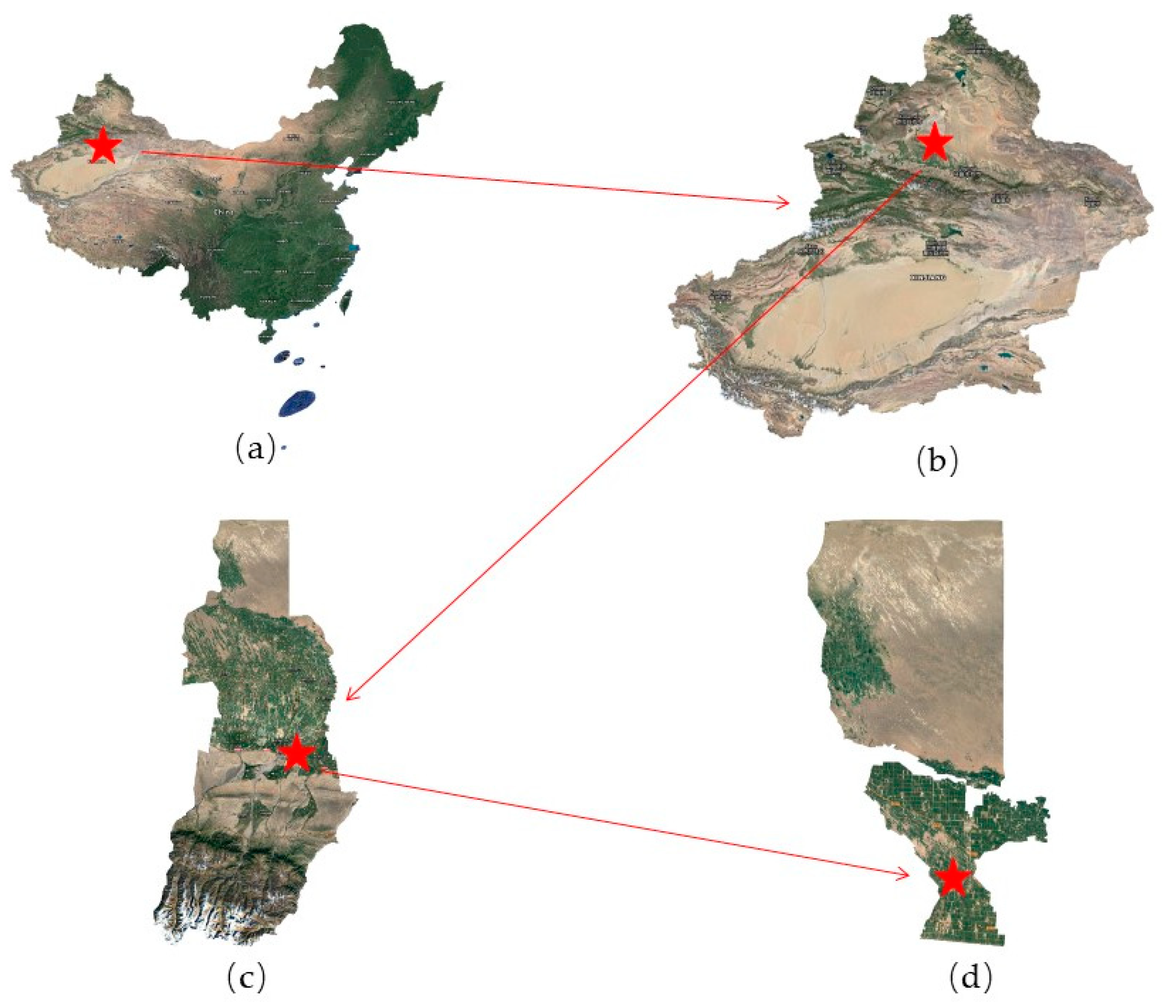
The experimental area was in the 122nd regiment of the 8th agricultural division of Xinjiang production and construction corps (~44°37′–44°48′ N, ~85°27′–85°41′ E), as shown in Figure 1. The annual average sunshine duration in the test area is 2862 h, and is hot in summer and cold in winter. The annual average temperature is 8.7 °C, with an extreme maximum temperature reaching 43.1 °C and an extreme minimum temperature reaching −42.3 °C. The test area experiences rapid cooling in September and October, longer winters, shorter springs and autumns, large temperature differences between day and night, abundant light and heat resources, average annual precipitation of 141.8 mm, and an average annual potential evaporation of 1826.2 mm. The test area was flat, and the soil texture was sandy loam. Due to the dry climate and strong evaporation on the ground in the test area, the salt contained in soil parent material and groundwater accumulates on the surface with the rise of capillary water in soil. In addition, improper irrigation, poor drainage, rising groundwater levels, and salt accumulation on the surface with the rise of water cause a secondary salinization process and form secondary saline soil. The soil electrical conductivity (EC 1:5) in the test area is basically between 2.57–5.79 mS·cm⁻¹, which belongs to a strong saline soil degree according to the classification standard of salinization.

2.2. Test Methods

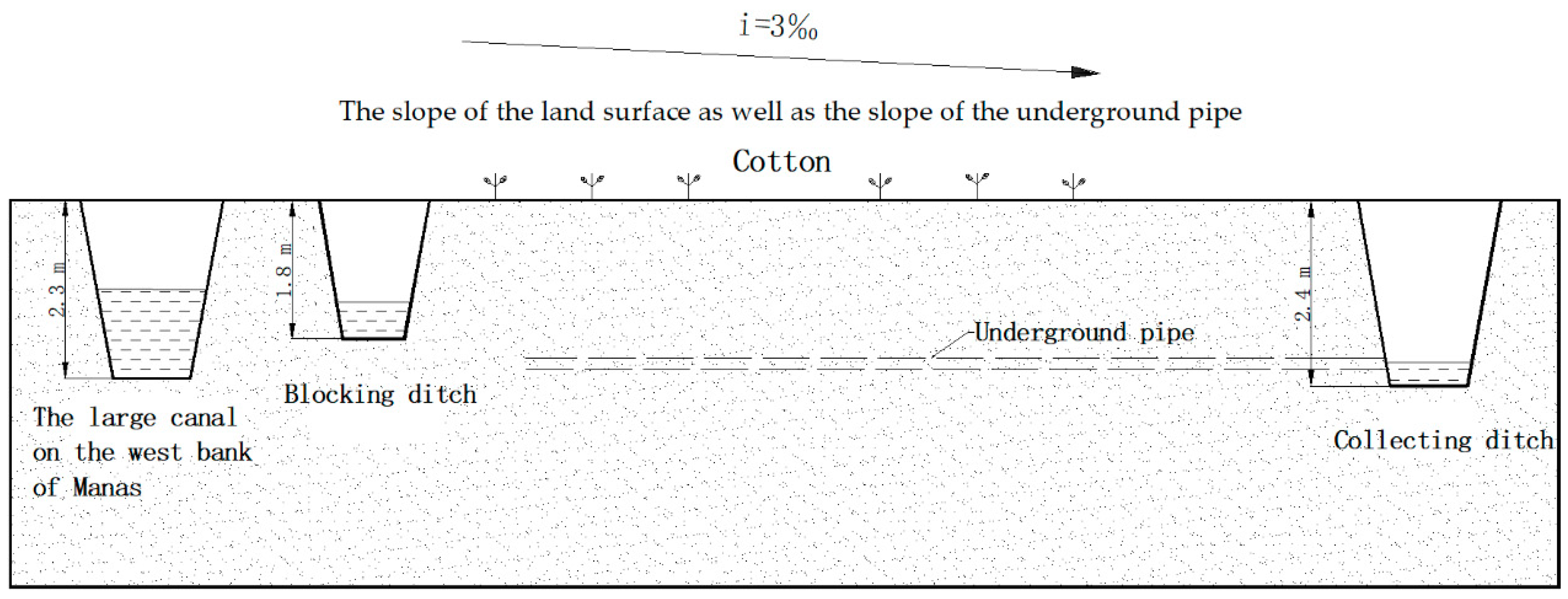
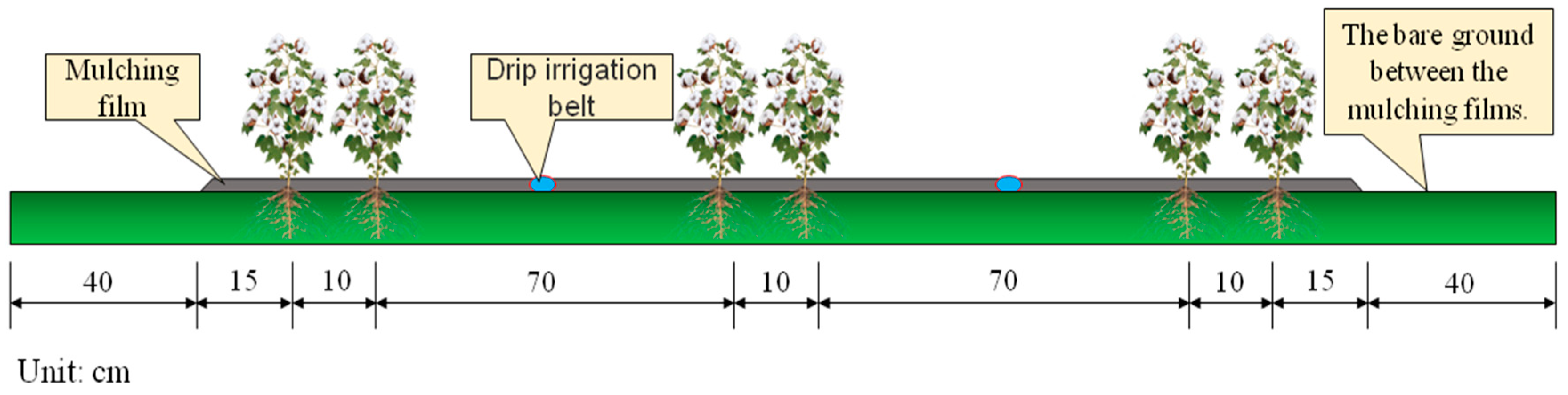
The pipe drainage system was used in the test area, and the water discharged from the underground pipe converged into the collecting ditch with a spacing of 48 m. Irrigation water was taken from the large canal on the west bank of Manas. There was a blocking ditch between the test area and the large canal to reduce the underground water level and decrease the influence of the large canal on the underground water level in the test area. A cross section of the test area is shown in Figure 2. In the experimental area, a single-wing labyrinth drip irrigation belt was used for irrigation. The dripper flow rate was 3.2 L/h. The distribution mode of the dripper was one mulching film, two tubes, and six rows. The mulching film was 0.015 mm thick, 2.2 m wide, and was placed 40 cm apart, as shown in Figure 3.

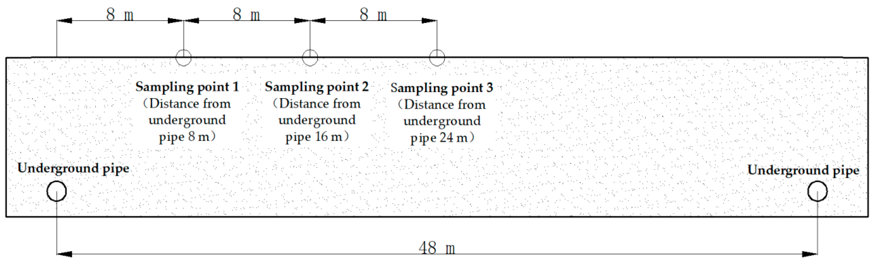
According to the observation wells, groundwater depth in the test area fluctuated during the irrigation season (April–October) between 1.75 and 2.1 m, and the groundwater depth during the non-irrigation season was below 2.2 m, as shown in

Table 1. Groundwater depth in each month in 2013.

Month	Groundwater Level/m
4	2.1
5	1.85
6	1.75
7	1.75
8	1.78
9	1.85
10	1.9

. The crops planted in this experiment were cotton, and drip irrigation under film was adopted. Cotton was sown on 15 April and harvested on 30 September. Samples were taken three times during the whole growth period. The HYDRUS model was used to simulate the salt transport during the whole growth period. The simulated values were verified by measured values. On this basis, we used the HYDRUS model to predict the return of salt in autumn. In this study, the reference crop evapotranspiration was calculated by the Penman–Monteith formula, and the crop water demand was estimated by Formula (1). The crop coefficient adopted the cotton standard crop coefficient recommended by FAO-56 (Food and Agriculture Organization of the United Nations), and then the irrigation schedule was determined according to the local irrigation experience, as shown in

Table 2. Irrigation schedule of test area.

Irrigation Date	Irrigation Quota/mm
04–20	180
05–01	60
06–01	60
06–21	60
06–31	60
07–11	60
07–21	60
07–31	60
08–11	60
08–21	60

. Winter snow cover in Xinjiang melts in early April, and the upper layer of soil becomes nearly saturated. To study the change in the salt discharge effect under drip irrigation leaching at different distances from the underground pipe, sampling points were set at 8, 16, and 24 m (Figure 4) to analyze the change in soil salinity. Three sampling points were set for each distance, and the distance between sampling points was 3 m. The sampling points were all in the film-covered area. According to the soil–water ratio of 1:5, the EC value of the soil sample was measured by DDS-11A (Shanghai Thunder Magnetic, Shanghai, China) digital conductivity meter.

In October 2012, a concealed pipe was buried in the field with an inner diameter of 70 mm and a buried depth of 2.2 m. The initial salt content of each sampling point was collected after sowing on 15 April 2013. In order to simplify the initial conditions of the model, the average salt content of each soil layer was calculated (

Table 3. The average initial salt content in different soil layers.

Soil Depth/cm	Initial Electrical Conductivity (EC 1:5)/(mS·cm−1)
0–20	6.06
20–60	5.26
60–100	4.72
100–140	3.64
140–160	3.91
160–200	3.91

). During the test, samples of each soil layer and pipe drainage water were collected on 25 May 2013, 20 July 2013, and 30 September 2013, taking into account the irrigation cycle and crop growth season. At sampling, twist drills were used to collect samples every 20 cm. The final depth of sampling was 200 cm. Pipe drainage water was sampled in three 500 ml bottles per sampling time, the salt contents were determined by drying, and the average value was taken. In our study, the “breakthrough curve (BTC)" was used to deduce the hydrodynamic dispersion coefficient. Breakthrough curve (BTC) refers to the curve of the relationship between the relative concentration [C(t) − C₀]/(C₁ − C₀) of a certain section and time or volume when air-dried soil samples are loaded into soil columns, the bulk density is strictly controlled, tracers are continuously and constantly injected into the soil, and then solute is transported in the soil. It is a basic curve reflecting solute transport in unsaturated soil. In addition, sodium chloride solution was used as tracer in this test.

2.3. Numerical Simulation

Model establishment: HYDRUS 2D/3D (PC-Progress, Prague, Czech Republic) software was used to simulate the soil salt movement in 2013. The width of the simulation region was 2470 cm. The model simulated the soil down to 200 cm, which was divided into 10–20 cm layers. The simulation period was 164 days, from 20 April 2013 to 30 September 2013. The time step was adjusted according to the number of convergence iterations using a variable time step subdivision method [20]. The soil hydraulic model adopted Van Genuchten–Mualem in the software.

The upper boundary of the model consisted of a film-covered area, a dripper area, and bare land between films. The film-covered area was set as a zero-flux boundary, the bare land between films was set as an atmospheric boundary, and the dripper area was set as a variable flow boundary. The underground pipe region was set as the permeation boundary, and the left, right, and lower boundaries were set as zero-flux boundaries.

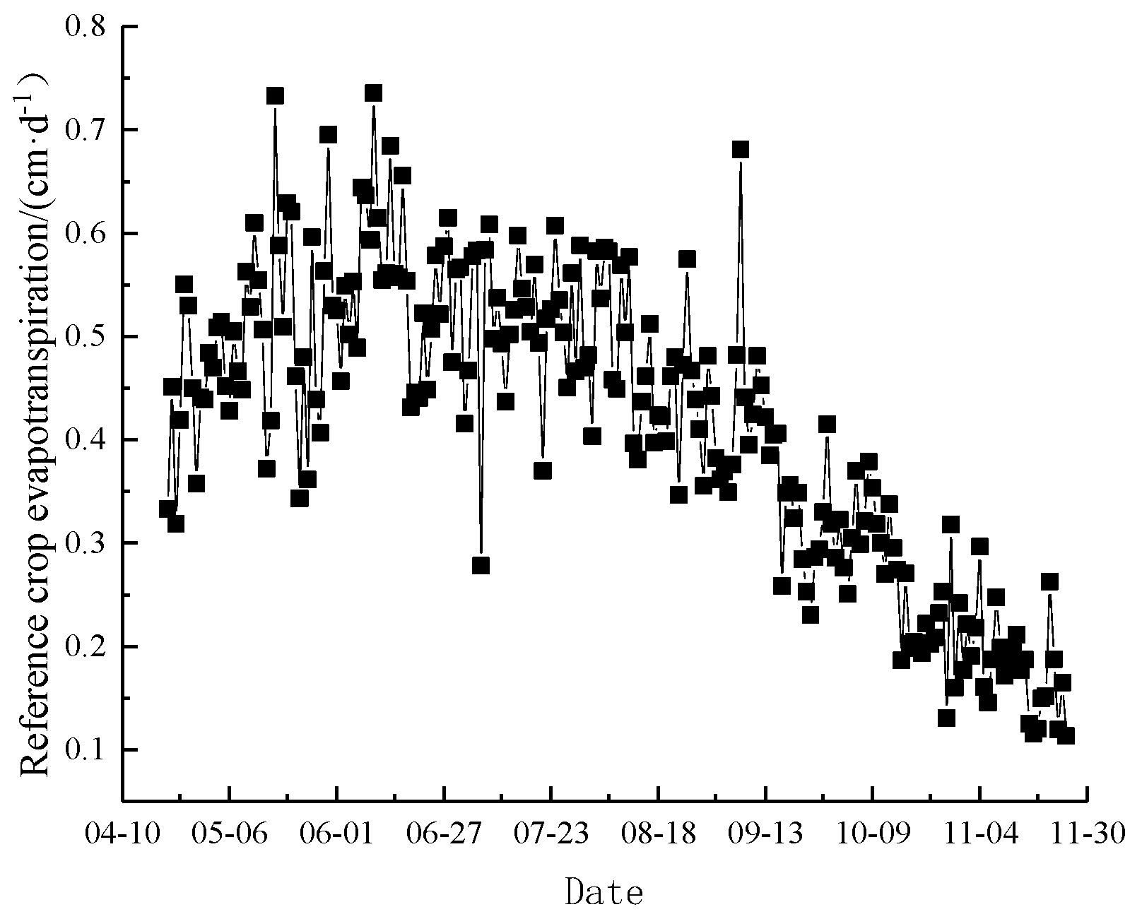
According to the measured the contents of clay, silt, and sand in the study area, the characteristic soil parameters were selected in the HYDRUS database (

Table 4. Characteristic parameters of soil.

Soil	Sandy Loam
$\gamma$/(g/cm3)	1.51
${\mathit{\theta }}_{\mathit{r}}$	0.065
${\mathit{\theta }}_{\mathit{s}}$	0.41
$\alpha$/(1/cm)	0.075
n	1.89
${\mathit{K}}_{\mathit{s}}$/(cm/d)	106.1
l	0.5

Note: $\mathit{\gamma }$ is the average soil bulk density; ${\mathit{\theta }}_{\mathit{r}}$ is the residual volume moisture content of soil; ${\mathit{\theta }}_{\mathit{s}}$ is the saturated volume moisture content of soil; $\alpha$ is a parameter related to soil physical properties; n is the empirical coefficient; ${\mathit{K}}_{\mathit{s}}$ is the saturated hydraulic conductivity of soil; $\mathit{l}$ is the parameter of porosity correlation.

). The software simulated drip irrigation under film, and the precipitation during the cotton growth period was small, so the influence of precipitation on water and salt transport was ignored. To obtain the best fit between measured and simulated values, the revised hydrodynamic dispersion coefficients were adjusted on the basis of the breakthrough curve (BTC), and the revised hydrodynamic dispersion coefficient (

Table 5. Hydrodynamic dispersion coefficient.

Soil	Disp. L	Disp. T
Sandy loam	20	4

Note: Disp. L is the longitudinal dispersion coefficient; Disp. T is the transverse dispersion coefficient.

) was given. The water uptake parameters of cotton root were shown in

Table 6. Root water uptake parameters.

P0/cm	P0pt/cm	P2H/cm	P2L/cm	P3/cm	Maximum Rooting Depth/cm	Depth of Maximum Intensity/cm	Threshold/cm	Slop
−10	−25	−200	−600	−14,000	60	25	15.4	2.6

Note: P0 is the negative pressure value when the soil void is completely filled with water; P0pt is the negative pressure value corresponding to the maximum amount of soil capillary rising water; P2 is the negative pressure value when soil capillary water breaks due to surface evaporation and crop absorption; P3 is the negative pressure value corresponding to permanent wilting of crops; Threshold is the value of the minimum osmotic head (the salinity threshold) above which root water uptake occurs without a reduction; Slop is the slope of the curve determining the fractional root water uptake decline per unit increase in salinity below the threshold.

according to previous research results [21]. The salinity stress response function adopted the Threshold Model in Multiplicative Model and selected Threshold and Slope values corresponding to cotton in the database of HYDRUS, as shown in Table 6. According to meteorological data from Paotai Meteorological Station, reference crop evapotranspiration was calculated according to the Penman–Monteith formula [22], as shown in Figure 5. Potential evaporation and potential transpiration were calculated according to Equations (1), (2), and (3). The mean square error (RMSE) was used to verify the reliability of the simulation results, whose calculation formula is Equation (4) [23,24].

$$E{T}_p=K_c\times E{T}_0$$

(1)

$$E_p=\frac{\Delta R_n}{L\left(\Delta +\gamma \right)}\times e^{-0.39LAI}$$

(2)

$$T_p=E{T}_p-E_p$$

(3)

where $E{T}_p$ is the potential evapotranspiration rate, cm·d⁻¹; $K_c$ is the crop coefficient of cotton; $E{T}_0$ is the reference crop evapotranspiration rate, cm·d⁻¹; $E_p$ is the potential evaporation rate, cm·d⁻¹; $T_p$ is the potential transpiration rate, cm·d⁻¹; $\Delta$ is the slope of saturated vapor pressure curve, kPa·°C⁻¹; $R_n$ is the net solar radiation, MJ/m² d; $L$ is the latent heat of vaporization of water, MJ kg⁻¹; $\gamma$ is the psychrometric constant, kPa·°C⁻¹, and LAI is leaf area index.

$$\mathrm{RMSE}=\sqrt{\frac{1}{n}{\displaystyle \sum }_{i=1}^n{\left(x_i-y_i\right)}^2}$$

(4)

where $x_i$ is the measured value; $y_i$ is analog value; n is the number of samples.

2.4. Model Application

To describe the distribution and dynamic change in salt in the root layer during the growth period and before the soil froze, we established a numerical model again on the basis of the above numerical simulation to simulate the return of salt in autumn. During salt return in autumn, the upper boundary of the model was set as the atmospheric boundary, and the precipitation and irrigation amounts were set to 0. The simulation was carried out under bare soil condition.

Observation nodes were respectively set under and between the mulching films of the numerical model, and the change of the average value of soil salinity was used to represent the change of the total salt in the whole simulation area.

2.5. Basic Equations of the Model

Considering the water uptake by crop roots, the equations used were as follows:

2.5.1. Soil Water Transport Equation

$$\frac{\partial \theta \left(h\right)}{\partial t}=\frac{\partial }{\partial x}\left[K\left(h\right)\frac{\partial h}{\partial x}\right]+\frac{\partial }{\partial z}\left[K\left(h\right)\frac{\partial h}{\partial z}\right]+\frac{\partial K\left(h\right)}{\partial z}-S$$

(5)

where $\theta \left(h\right)$ is the volume moisture content of soil, cm³·cm⁻³; h is the pressure head, cm; $K\left(h\right)$ is unsaturated soil hydraulic conductivity, cm·d⁻¹; t is time, x is transverse coordinate, z is vertical coordinate, and provide that z is positive upward; S is the source and sink term, which means the water absorption rate of the root system, that is, the volume of water absorbed by the root system in unit volume of soil in unit time, d⁻¹.

2.5.2. Van Genuchten Formula for Soil Hydraulic Function

$${\theta }_e=\frac{\theta \left(h\right)-{\theta }_r}{{\theta }_s-{\theta }_r}={\left(1+{\left|\alpha h\right|}^n\right)}^{-m}$$

(6)

$$K\left(\theta \right)=K_s{\theta }_e^l{\left[1-{\left(1-{\theta }_e^{\frac{1}{m}}\right)}^m\right]}^2$$

(7)

where $K_s$ is saturated hydraulic conductivity of soil, cm·d⁻¹; ${\theta }_e$ is relative saturation of soil; ${\theta }_r$ is the residual volume moisture content of soil; ${\theta }_s$ is the saturated volume water content of soil; n, m, and α are all empirical parameters. Among them, m = 1 − 1/n, and α is a parameter related to soil physical properties; $l$ is the parameter of porosity correlation, and the average value is usually 0.5.

2.5.3. Basic Equation of Salt Transport in the Model

$$\frac{\partial \left(\theta c\right)}{\partial t}=\frac{\partial }{\partial x_i}\left(\theta D_{ij}\frac{\partial c}{\partial x_i}\right)-\frac{\partial \left(q_{i}c\right)}{\partial x_i}-S{C}_s$$

(8)

where c is solute concentration, g·cm⁻³; $q_i$ is the infiltration rate, cm·d⁻¹; $D_{ij}$ is the dispersion coefficient, cm²·d⁻¹; $x_i$ is the spatial coordinate (I = 1,2), $x_1=x$, $x_2=z$, $D_{11}=D_{xx}$, $D_{12}=D_{xz}$; $C_{\mathrm{s}}$ is the sink salt content, g·L^−1..

2.5.4. Root Water Absorption Adopts the Modified Feddes Model

$$S\left(h,h_{\phi },x,z\right)=\alpha \left(h,h_{\phi },x,z\right)b\left(x,z\right)S_t{T}_p$$

(9)

where $\alpha \left(h,h_{\phi },x,z\right)$ is the soil water and salt stress function; $h_{\phi }$ is osmotic pressure, cm; $b\left(x,z\right)$ is the root distribution function, cm⁻²; $S_t$ is the surface length associated with transpiration, cm; $T_p$ is the potential transpiration rate, cm·d⁻¹.

3. Results

3.1. Analysis of Measured Salt Data

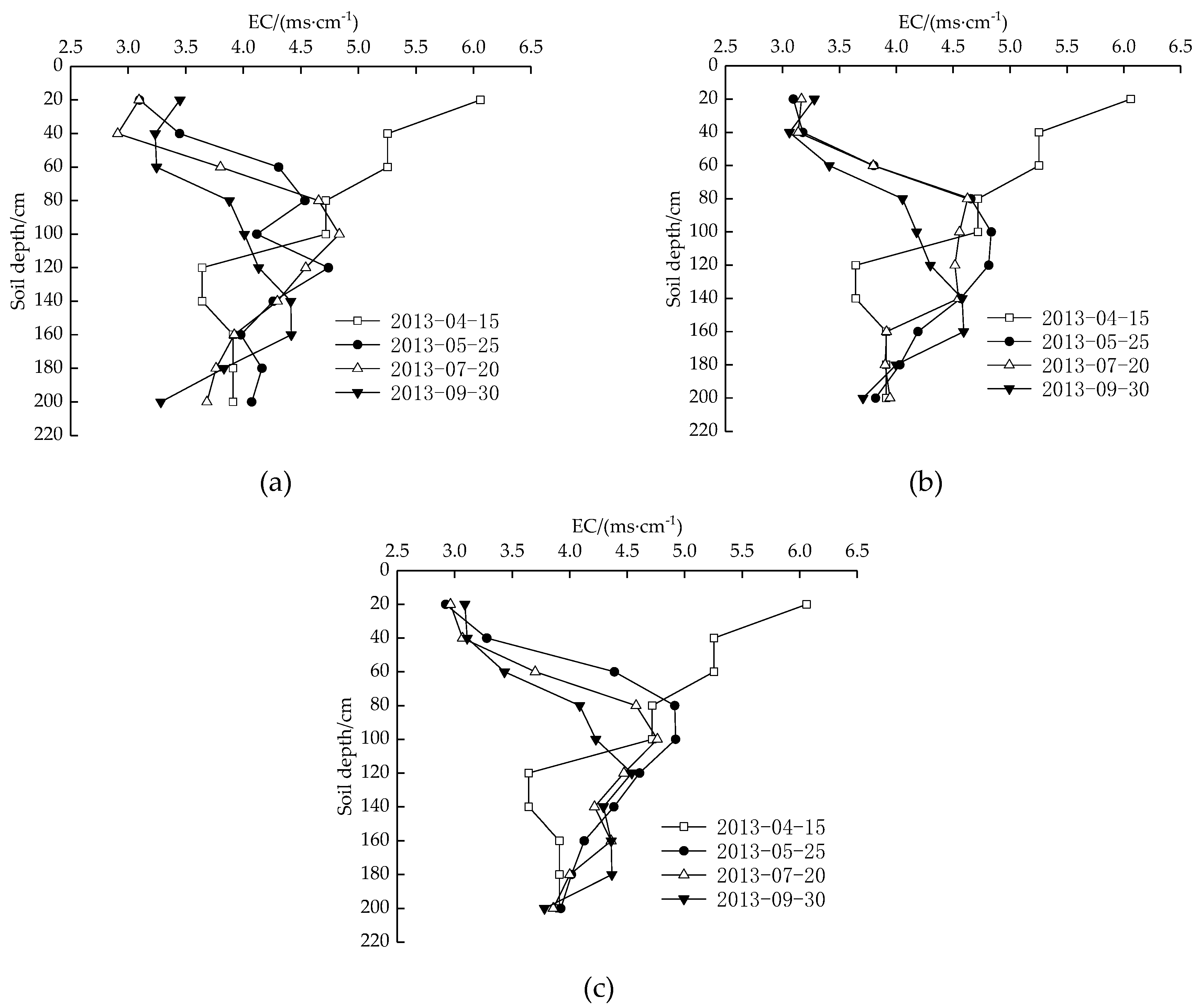
From Figure 6, compared with the initial salt content, soil salinity evidently decreased within the depth range of 0–80 cm. With the increase in soil depth, the decrease degree of soil salinity gradually decreased. In the depth range of 80–200 cm, the soil salt content gradually changed from decreasing to increasing compared with the initial salt content. The peak value of soil salt content gradually migrated downward throughout the cotton growth period and finally migrated from 80–100 cm to 140–160 cm soil depth. This showed that while salt moved downward with irrigation water, the upper soil salt supplemented the lower soil salt.

The salt content at a depth of 20 cm on 30 September was higher than that on 25 May and 20 July. This was because after film mulching was removed in late September, soil salt accumulated on the soil surface again due to strong evaporation.

The average salinity of water samples from pipe drainage, measured three times, was 92.8 g/L. The salinity of groundwater and irrigation water samples obtained from observation wells and west bank canals was 10.3 g/L and 0.96 g/L, respectively, which were far less than the salinity of water samples discharged from underground pipes. This shows that most of the salt discharged from the underground pipe comes from soil. Long-term use of pipe drainage can alleviate the salt accumulation caused by drip irrigation under film.

3.2. Verification of Numerical Model

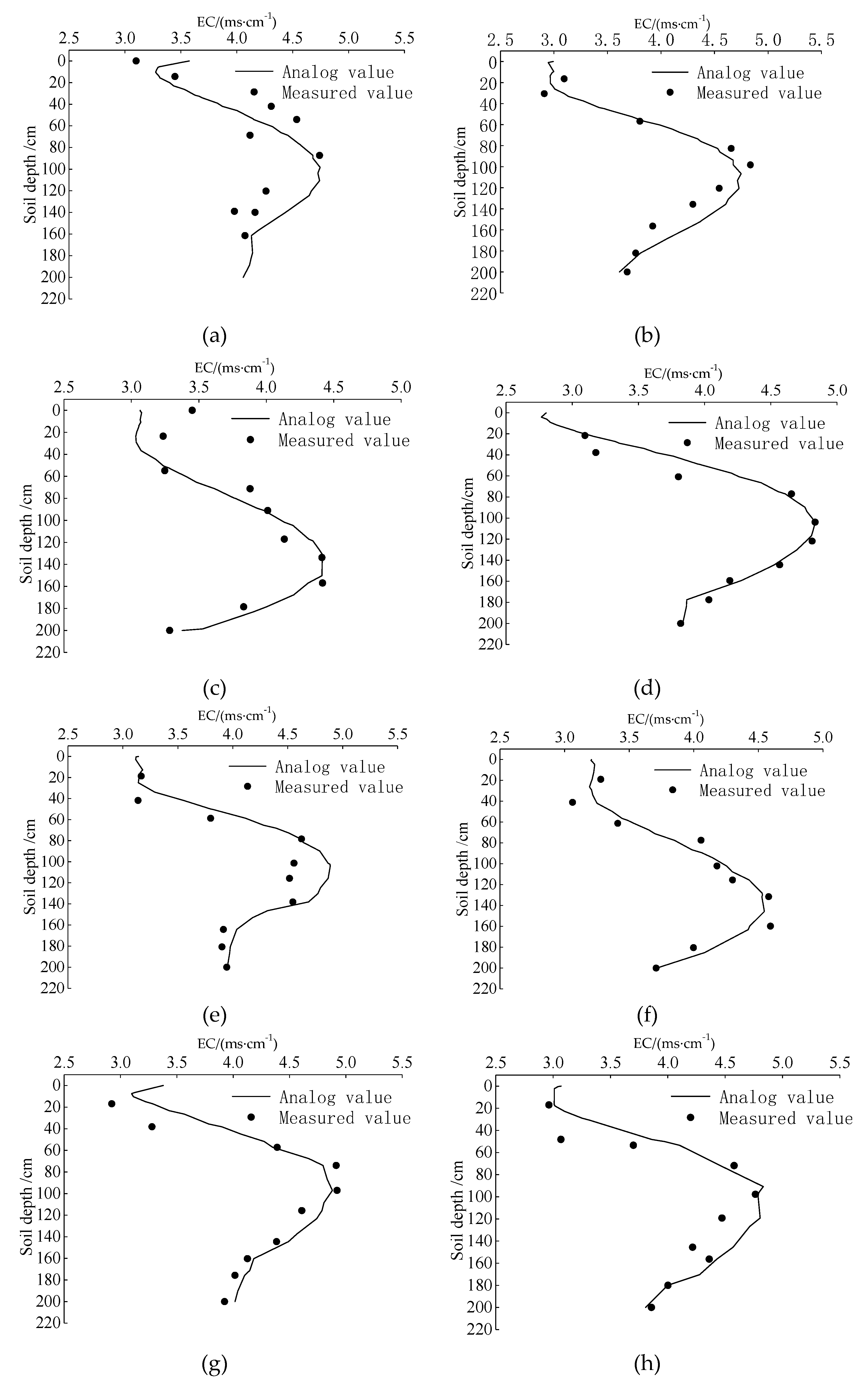
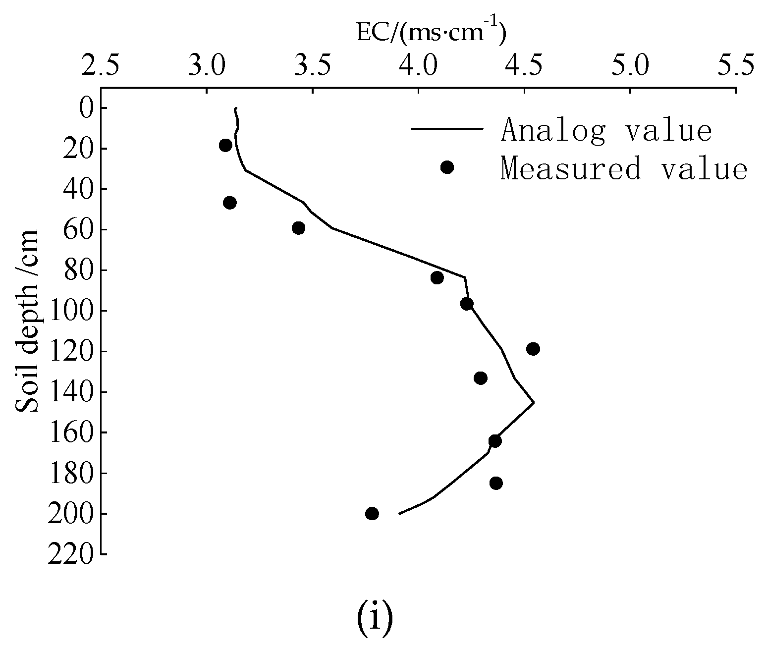
Figure 7 shows the comparison between the simulated value and the measured value of soil salinity. The simulated values were in good agreement with the measured values.

From

Table 7. Mean square error (RMSE) value between measured value and simulated value.

A/(mS·cm−1)	B/(mS·cm−1)	C/(mS·cm−1)
0.1954	0.1274	0.1357

Note: A is the RMSE value between measured and simulated salt values of all soil samples collected from sampling point 1; B is the RMSE value between measured and simulated salt values of all soil samples collected from sampling point 2; C is the RMSE value between measured and simulated salt values of all soil samples collected from sampling point 3.

and

Table 8. Correlation between measured and simulated values.

A	B	C
0.8107	0.8977	0.8649

Note: A is the correlation between measured and simulated salt values of all soil samples collected from sampling point 1; B is the correlation between measured and simulated salt values of all soil samples collected from sampling point 2; C is the correlation between measured and simulated salt values of all soil samples collected from sampling point 3.

, it can be seen that RMSE of simulated and measured values at different distances were smaller, R² was larger, and the fitting effect was better, which shows that the measured and simulated values of soil salinity at different distances were not considerably different, and the parameters were more reliable.

3.3. Model Application Results

3.3.1. Analysis of Salt Changes with Time

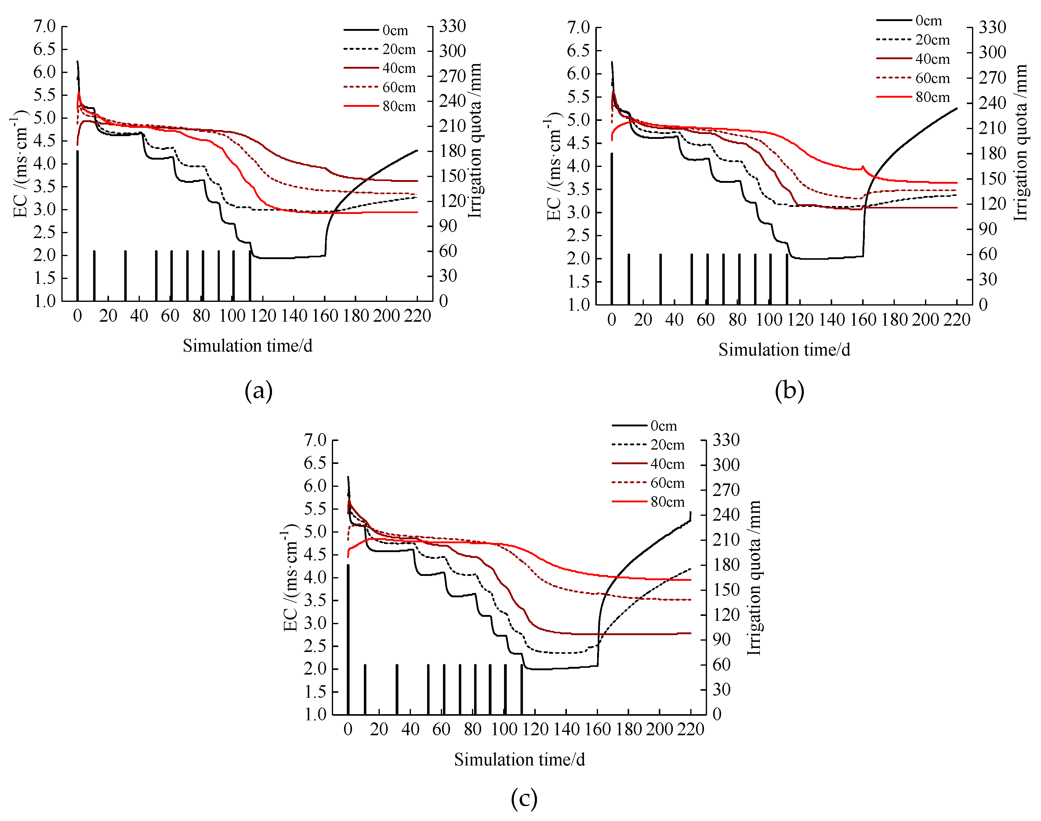
Figure 8 is a graph showing the change in salinity in the 0–80 cm soil layer over time, taking the film-covered area as the sampling point. It could be seen that the soil salt content in the root layer of cotton decreased during the whole growth period, and the degree of decrease decreased as soil depth increased. The average soil salt content (EC 1:5) in the surface layer decreased by 67.32%, in the 20 cm soil layer by 48.58%, in the 40 cm soil layer by 46.22%, in the 60 cm soil layer by 22.68%, and in the 80 cm soil layer by 17.18%.

After the mulching film was removed in late September, the soil salt content in the surface layer of the soil increased rapidly due to evaporation, and the soil salt content in the 40–80 cm soil layer did not change significantly (from the 160th day to the 220th day in Figure 8). Soil froze in the test area in late November, before which the soil salt content (EC 1:5) in the surface layer of the soil increased to between 4.18 and 5.26 mS·cm⁻¹, while the salt content (EC 1:5) in the soil below 40 cm depth basically did not change after it decreased to between 3.11 and 4.18 mS·cm⁻¹ (Figure 8).

3.3.2. Analysis of Desalination Rate of Root Layer

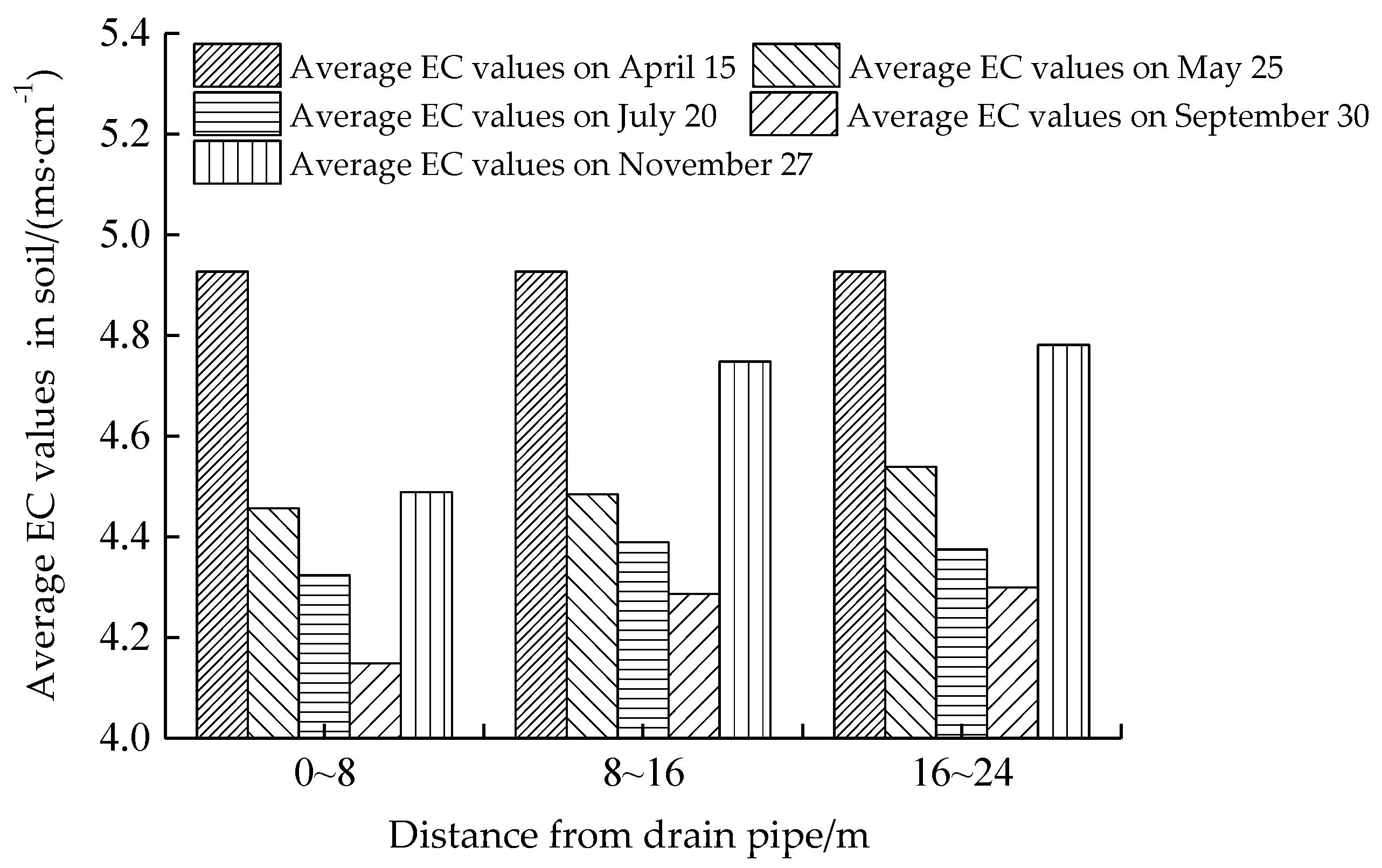
Figure 9 shows a graph illustrating the change in average EC values (in and between the mulching films) at a depth of 0–80 cm and a distance of 0–8, 8–16, and 16–24 m from the underground pipe. The desalinization rate of soil at the seedling stage (on 25 May) was 9.53%, 8.95%, and 7.85%, respectively, compared with that before sowing (on 15 April). Compared with the seedling stage (on 25 May), the desalinization rate of soil in the flowering stage (on 20 July) was 2.98%, 2.13%, and 3.62%, respectively. Compared with the flowering stage (on 20 July), the desalinization rate of soil at the harvest stage (on 30 September) was 4.05%, 2.35%, and 1.72%, respectively. Compared with the harvest period (on 30 September), soil salinity increased by 8.21%, 10.78%, and 11.19%, respectively, before the soil froze (on 27 November). During the growth period of cotton, the desalinization rate of soil in the depth range of 0–80 cm gradually decreased, and the desalinization rate in the early stage was much higher than that in the late stage. With the increase in distance from the underground pipe, the desalinization rate of soil tended to decrease. This shows that desalinization mainly occurred in the stage of irrigation and salt washing. During the salt returning stage in autumn, the soil salinity increased gradually in the depth range of 0–80 cm, and the degree of increase in soil salinity at 0–8 m was less than those at 8–16 m and 16–24 m.

3.3.3. Analysis of Desalination Rate at Depth of 0–200 cm

Figure 10 shows a graph illustrating the change in average EC values (in and between the mulching films) at a depth of 0–200 cm and a distance of 0–8, 8–16, and 16–24 m from the underground pipe. It could be seen that the average EC values of the soil decreased after the salt returning stage in autumn, which indicated that the underground pipe discharged salt. Compared with before sowing (on 15 April), the average EC values before the soil froze (on 27 November) decreased by 3.03%, 2.48%, and 2.36% (0–8, 8–16, and 16–24 m, respectively). The amount of salt discharged from 0–8 m soil mass was larger than that of the latter two soil masses, and the amount of salt discharged from the latter two soil masses was not considerably different.

4. Discussion

Pan [24], Zhang [25], Tan [26], Li [27], and Yang [28] found that, when the irrigation quota was large enough, the salt content in the upper soil decreased, while the salt content in the wet front of the soil increased due to the downward migration of salt from the upper soil with the irrigation water. This study also found that during the growth period of cotton, after irrigation, the upper layer salt will migrate downward. Along with the growth period of cotton, the peak value of soil salt content also gradually migrated downward and eventually migrated from 80–100 cm to 140–160 cm soil depth. Sulitan et al. [29], through the experimental study of soil water and salt transport under drip irrigation under film, reported that, after irrigation, soil salt presented a two-way migration trend from the deep soil to the surface and from under film to between films, and did not continue to migrate downward. Our results do not agree with Sulitan’s results in that during the growth period of cotton, after irrigation, because pipe drainage controls the groundwater level, the salt in the upper layer of the soil will continue to migrate downward along with the water. In late September, the cotton field became bare. Under the action of evaporation, the salt content in the surface soil increased rapidly, while the salt content in the soil layer below 40 cm did not change significantly.

Pipe drainage measures can effectively control the underground water level and drain soil salt. Zhang et al. [30] reported that the desalinization rate of the 0–30 cm soil layer was 74.8–95.4% at the buried depth of the pipes (1.2 m) after leaching for 43 days by flood irrigation under pipe drainage. Heng et al. [31] conducted field irrigation and drainage tests based on different buried depths and pipe diameters. The results showed that the desalination effect of 0.6 m depth of buried pipe was higher than that of 1.0 and 1.4 m depths, with the average desalting rate reaching 57.04%. The results of the present study showed that in the 0–80 cm soil layer, the average desalinization rate reached 43.52% under the mulching films, and the average desalinization rate reached 13.83% under and between the mulching films compared with that before sowing, which was less than the above studies.

There were two main reasons for these discrepancies. On the one hand, the depth of the soil layer was different, and the desalinization rate of the soil would decrease with increasing soil depth. On the other hand, the buried depths of the underground pipes were different, and shallow burial of underground pipes would increase the desalinization efficiency of the soil layer above the underground pipes. However, the salt was not completely drained by the underground pipes, and a larger part was leached to the soil layer below the underground pipes. In addition, indicators such as underground pipe spacing, soil type, crop planting mode, and irrigation schedule would also affect the desalinization rate of each soil layer.

Many studies [13,32,33] have shown that the desalinization rate of soil at different sections is inversely proportional to the distance from the underground pipe. The closer to the underground pipe, the greater the desalinization rate, and the farther from the underground pipe, the smaller the desalinization rate [34,35]. This is similar to our research, but the difference is that the average desalinization rate of 0–8 m soil is greater than that of 8–16 m and 16–24 m soil, but the difference between the latter two is very small.

After returning salt in autumn, the average EC value at 0–200 cm soil depth decreased by 2.60% on average compared with that before sowing. This further showed that most of the salt was leached to the lower layer of soil. Some remained in the soil and some dissolved in groundwater and were drained by the underground pipes. However, the total amount of salt in the soil of this model will continuously decrease after long-term use.

5. Conclusions

The combination of drip irrigation under film and pipe drainage has made the desalination effect of the soil root layer prominent. The simulated values obtained by the HYDRUS 2D/3D software were in good agreement with the measured values. The maximum RMSE and minimum R² of soil salinity were 0.1954 mS·cm⁻¹ and 0.8107, respectively, which were within the acceptable range.

Under the conditions of pipe drainage and drip irrigation under film, compared with before sowing, the average desalinization rate reached 43.52% under the mulching films in the 0–80 cm soil layer, and the average desalinization rate reached 13.83% under and between the mulching films. After the cotton harvest, the salt content in the upper layer of the soil increased, and compared with the harvest period before the soil froze, the salt content in 0–80 cm soil increased by 10.06% on average.

Compared with before sowing, salt content at 0–80 cm soil depth decreased by 5.14% on average after salt inversion in autumn, and salt content at 0–200 cm soil depth decreased by 2.60% on average, which indicates that the total amount of salt in the soil will continuously decrease after long-term use of drip irrigation and salt drainage by underground pipes.

In this experiment, 10 instances of irrigation were conducted, and the irrigation quota was 720 mm. The first irrigation amount was 180 mm, and the irrigation amount was 60 mm every 10 days in every growth period (except for the seedling period) of cotton. The results show that the irrigation schedule can not only meet the water demand of cotton, but also achieve the purpose of drainage and salt discharge from underground pipes.

References

- Wang, Q.J.; Wang, W.Y.; Lu, D.Q. Water and Salt Transport Features for Salt-Effected Soil Through Drip Irrigation Under Film. Trans. Chin. Soc. Agric. Eng. 2000, 16, 54–57. [Google Scholar]
- Tian, F.Q.; Wen, L.; Hu, H.C. Review on water and salt transport and regulation in drip irrigated fields in arid regions. J. Hydraul. Eng. 2018, 49, 126–135. [Google Scholar]
- Wang, R.S.; Wan, S.Q.; Sun, J.X. Soil salinity, sodicity and cotton yield parameters under different drip irrigation regimes during saline wasteland reclamation. Agric. Water Manag. 2018, 209, 20–31. [Google Scholar] [CrossRef]
- Meng, C.R.; Yan, L.; Zhang, S.J. Variation of Soil Salinity in Plow Layer of Farmlands under Long-term Mulched Drip Irrigation in Arid Region. Acta Pedol. Sin. 2017, 54, 1386–1394. [Google Scholar]
- Liu, X.Y.; Tian, C.Y. Study on Dynamic and Balance of Salt for Cotton under Plastic Mulch in South Xinjiang. J. Soil Water Conserv. 2005, 19, 82–85. [Google Scholar]
- Mu, H.C.; Hudan, T.; Su, L.T. Experimental Research on Salty Soil Profile Transfer Law under Different Farming Times. Water Sav. Irrig. 2011, 8, 29–31. [Google Scholar]
- Yi, P.F.; Hudan, T.; Wu, Z.G. Research on Soil Salt Accumulation Influence by the Years of Covered Cotton under Drip Irrigation. Res. Soil Water Conserv. 2010, 17, 118–122. [Google Scholar]
- Gao, C.Y. Gutter drainage and vertical drainage of groundwater. Ground Water 2001, 23, 194–197. [Google Scholar]
- Ma, L.J.; Wang, H.Y.; Mai, W.H. Investigation and Analysis of Application of Underground Pipe Drainage Technology in Yinbei Irrigation Area of Ningxia. China Rural Water Hydropower 2019, 2, 71–79. [Google Scholar]
- Tan, L.M.; Liu, J.T.; Liu, H.T. Study on the adaptability and potential application effects of subsurface pipe drainage system in the coastal areas of Hebei Province. Chin. J. Ecol.-Agric. 2012, 20, 1673–1679. [Google Scholar] [CrossRef]
- Mehdi, J.T.; Abdullah, D.N.; Lotfullah, Z.P. Investigating long-term effects of subsurface drainage on soil structure in paddy fields. Soil Till. Res. 2018, 177, 155–160. [Google Scholar]
- Xu, Y.X.; Yu, S.H.; Shi, L. Effects of subsurface controlled drainage on reducing salinity and preventing basification in saline-alkali areas with underground high water level. J. Arid Land Resour. Environ. 2018, 32, 164–169. [Google Scholar]
- Ji, J.H.; Wang, H.Y. Monitoring and analysis of salinity and alkalinity of soil under the condition of underground pipe drainage. Ningxia Eng. Technol. 2018, 17, 71–75. [Google Scholar]
- Mai, W.H.; Wang, H.Y.; Ma, L.J. Calculation Method Research on Pipe Drain Spacing of Ningxia Yellow River Irrigation Region Based on VBA. J. Irrig. Drain 2019, 38, 64–72. [Google Scholar]
- Shi, P.J.; Liu, H.G.; He, X.L. The simulation of water and salt transportation under subsurface drainage by HYDRUS model. Agric. Res. Arid Areas 2019, 37, 224–231. [Google Scholar]
- Geng, Q.M.; Yan, H.H.; Yang, J.Z. Evaluation for Soil Improvement Effect of Open Ditch and Concealed Drainage Engineering on Saline Alkali Land Development. Chin. J. Soil Sci. 2019, 50, 617–624. [Google Scholar]
- Zhang, Z.Y.; Zhang, Y.Z.; Zhang, J. Simulating subsurface pipe drainage in saline-alkali farmland along coastlines using the DRAINMOD-S model. Adv. Water Sci. 2012, 23, 782–788. [Google Scholar]
- Adobea, M.A.; Ramanathan, S.R.; Paul, B. Subsurface drainage for promoting soil strength for field operations in southern Manitoba. Soil Till. Res. 2018, 184, 261–268. [Google Scholar]
- Li, X.W.; Zuo, Q.; Shi, J.C. Evaluation of salt discharge by subsurface pipes in the cotton field with film mulched drip irrigation in Xinjiang, ChinaⅠ. Calibration to models and parameters. J. Hydraul. Eng. 2016, 47, 537–544. [Google Scholar]
- Yu, G.J.; Huang, J.H.; Gao, Z.Y. Study on water and salt transportation of different irrigation modes by the simulation of HYDRUS model. J. Hydraul. Eng. 2013, 44, 826–834. [Google Scholar]
- Wang, Z.M. Study on the Cotton-Water-Solute Interactions under Mulched Drip Irrigation with Brackish Water in an Arid Area; China University of Geosciences: Wuhan, China, 2013. [Google Scholar]
- Monteith, J.L. Evaporation and environment. Symp. Soc. Exp. Biol. 1965, 19, 205–234. [Google Scholar]
- Yang, S.Q.; Ding, X.H.; Jia, J.F. Light-saline water use pattern in saline soil environment. J. Hydraul. Eng. 2011, 42, 490–498. [Google Scholar]
- Pan, Y.X.; Luo, W.; Jia, Z.H. The simulation of water and salt transportation by HYDRUS model in Lubotan of Shaanxi, China. Agric. Res. Arid Areas 2017, 35, 135–142. [Google Scholar]
- Zhang, W.; Lv, X.; Li, L.H. Salt transfer law for cotton field with drip irrigation under the plastic mulch in Xinjiang Region. Trans. Chin. Soc. Agric. Eng. 2008, 24, 15–19. [Google Scholar]
- Tan, J.L.; Kang, Y.H.; Jiao, Y.P. Characteristics of soil salinity and salt ions distribution in salt-affected field under mulch-drip irrigation in different planting years. Trans. Chin. Soc. Agric. Eng. 2008, 24, 59–63. [Google Scholar]
- Li, M.S.; Liu, H.G.; Zheng, X.R. Spatiotemporal variation for soil salinity of field land under long-term mulched drip irrigation. Trans. Chin. Soc. Agric. Eng. 2012, 28, 82–87. [Google Scholar]
- Yang, P.N.; Dong, X.G.; Liu, L. Soil salt movement and regulation of drip irrigation under plastic film in arid area. Trans. Chin. Soc. Agric. Eng. 2011, 27, 90–95. [Google Scholar]
- Su, L.T.; Abudu, S.; Song, Y.D. Effects of drip irrigation volume on soil water-salt transfer and itsredistribution. Arid Zone Res. 2011, 28, 79–84. [Google Scholar] [CrossRef]
- Zhang, J.L.; Liu, M.; Qian, H. Spatial-temporal variation characteristics of water-salt movement in coastal saline soil improved by flooding and subsurface drainage. Trans. Chin. Soc. Agric. Eng. 2018, 34, 98–103. [Google Scholar]
- Heng, T.; Wang, Z.H.; Li, W.H. Impacts of Diameter and Depth of Drainage Pipes in Fields under Drip Irrigation on Soil Salt. Acta Pedol. Sin. 2018, 55, 111–121. [Google Scholar]
- Zhang, J.; Chang, T.T.; Shao, X.H. Improvement effect of subsurface drainage on secondary salinization of greenhouse soil and tomato yield. Trans. Chin. Soc. Agric. Eng. 2012, 28, 81–86. [Google Scholar]
- Wang, H.Y.; Wang, Z.H.; Yang, F.J. Research for the Effect of Shallow-Tight Type Subsurface Drain pipes on Improving Soda Saline-alkaline land. Res. Soil Water Conserv. 2013, 20, 269–272. [Google Scholar]
- Zheng, W.Z.; Huang, J.S.; Xie, H. Analysis of nitrate-nitrogen loss under different underground pipe layout. Trans. Chin. Soc. Agric. Eng. 2012, 28, 89–93. [Google Scholar]
- Chen, Y.; Zhang, J.Y.; Feng, G.X. Desalination of Subsurface Pipe Drainage in Saline-alkali Land of Coastal Areas. J. Irrig. Drain 2014, 33, 38–41. [Google Scholar]
Figure 1.
Maps of research area. (a) China; (b) Xinjiang Uygur Autonomous Region; (c) Tacheng Area; (d) Shawan County. Note: The red five-pointed star represents the area indicated by the red arrow, and the last red five-pointed star represents the location of the test area.
Figure 2.
Sectional drawing of test area.
Figure 3.
Diagram of drip irrigation system layout.
Figure 4.
Schematic of sampling points.
Figure 5.
Reference crop evapotranspiration in researched region.
Figure 6.
Characteristic diagram of salt distribution under drainpipe drainage. (a) Distance from drainpipe 8 m; (b) distance from drainpipe 16 m; (c) distance from drainpipe 24 m.
Figure 7.
Comparison of simulated and measured values of soil salinity. (a) Distance from drainpipe 8 m (May 2013); (b) distance from drainpipe 8 m (July 2013); (c) distance from drainpipe 8 m (September 2013); (d) distance from drainpipe 16 m (May 2013); (e) distance from drainpipe 16 m (July 2013); (f) distance from drainpipe 16 m (September 2013); (g) distance from drainpipe 24 m (May 2013); (h) distance from drainpipe 24 m (July 2013); (i) distance from drainpipe 24 m (September 2013).
Figure 8.
Variation in salt content at 0–80 cm through time. (a) Distance from drainpipe 8 m; (b) distance from drainpipe 16 m; (c) distance from drainpipe 24 m.
Figure 9.
Variation of average EC values at 0–80 cm in simulated area.
Figure 10.
Variation of average EC values at 0–200 cm in simulated area.