New Approach to Improve the Soil Water Balance Method for Evapotranspiration Estimation


Department of Agricultural and Biosystems Engineering, North Dakota State University, Fargo, ND 58102, USA
*
Author to whom correspondence should be addressed.
Water 2019, 11(12), 2478; https://doi.org/10.3390/w11122478
Submission received: 25 October 2019
/
Revised: 16 November 2019
/
Accepted: 20 November 2019
/
Published: 24 November 2019
(This article belongs to the Section Hydrology)
Abstract
:As an important component of the water budget, quantifying actual crop evapotranspiration (ET) will enable better planning, management, and allocation of the water resources. However, accurate ET measurement has always been a challenging task in agricultural water management. In the upper Midwest, where subsurface drainage is a common practice due to the shallow ground water depth and heavy clayey soil, ET measurement using traditional ground-based methods is more difficult. In this study, ET was measured using the eddy covariance (EC), Bowen ratio-energy balance (BREB), and soil water balance (SWB) methods during the 2018 corn growing season, and the results of the three methods were compared. To close the energy balance for the EC system, the residual method was used. For the SWB method, capillary rise was included in the ET estimation and was calculated using the measured soil water potential. The change of soil water content for ET estimation using the SWB method was calculated in four different ways, including daily average, 24:00–2:00 average, 24:00–4:00 average, and 4:00 measurement. Through the growing season, six observation periods (OPs) with no rainfall or minimal rainfall events were selected for comparisons among the three methods. The estimated latent heat flux (LE) by the EC system using the residual method showed a 29% overestimation compared to LE determined by the BREB system for the entire growing season. After excluding data taken in May and October, LE determined by the EC system was only 10% higher, indicating that the main difference between the two systems occurred during the early and late of the growing season. By considering all six OPs, a 6%–22% LE difference between the EC and the BREB systems was observed. Except during the early growing and late harvest seasons, both systems agreed well in LE estimation. The SWB method using the average soil water contents between 24:00 and 2:00 time period to calculate the daily capillary rise produced the best statistical fit when compared to the ET estimated by the BREB, with a root-mean-square error of 1.15. Therefore, measuring ET using the capillary rise from a shallow water table between 24:00 and 2:00 could improve the performance of the SWB methodology for ET measurement.
1. Introduction
Precise estimates of actual crop evapotranspiration (ET) are crucial for the understanding of land and atmosphere energy exchange, especially for agricultural production. Knowledge about measurement techniques and their related errors is essential for agricultural water management. Over the last decade, development of instrumentation, data acquisition systems, and remote sensing have enhanced the ability of ET measurement over large areas and have significantly intensified the knowledge of ET measurement [1]. Numerous methods and techniques are now being used either remotely [2] or in situ (e.g., eddy covariance, Bowen ratio, soil water balance, and lysimeter) [3,4,5] for ET estimations. However, most of the ET methods, developed ET models, or proposed ET equations have large discrepancies and exhibit systematic and random errors depending on the measurement device’s location and climate conditions [6]. Despite the development of many methods and equations through past decades, accurate ET estimation is still a challenging task [7], and more efforts is required to increase our knowledge and the benefits of the available methods, while limiting their drawbacks.
In the upper Midwest, where subsurface drainage is a common practice due to the shallow ground water depth and heavy clayey soil, ET measurement is usually conducted using the soil water balance (SWB) method. However, due to the existence of a shallow water table, the accuracy of estimated ET with the SWB method is in doubt. To examine the performance of the SWB method, more precise instrumentation is needed. The eddy covariance (EC) and Bowen ratio-energy balance (BREB) systems are the two dominant in situ measurement methods that can provide ET with finer resolution compared with the SWB method. Furthermore, the results from the EC and the BREB methods may be used to improve the accuracy of the SWB method in the Red River Valley (RRV) region with a shallow water table and heavy clayey soil.
The EC method is one of the most established techniques to determine the exchange of water, energy, and trace gases between the land surface and the atmosphere [8]. The EC method measures the covariance between vertical wind speed and water vapor density and aims to calculate the vertical moisture flux (and thus, ET) in high frequency [9]. With the development of flux measurements, the use of EC is extending rapidly to more heterogenous stands [10,11], and this method has been compared with other ET methods [12]. Gebler et al. [9] showed a good correlation between ET values measured by lysimeter and EC in the summer. However, the comparison of ET values determined by the EC and other methods is poorly documented for regions with a shallow water table and heavy clay soil.
The BREB method, which is considered a fairly robust and successful tool in ET estimation, depends on the energy balance between the surface energy fluxes and the gaseous properties of water vapor [8,13]. Bowen ratio, which is the ratio of the sensible heat flux (H) to the latent heat flux (LE), operates on the basis of the concept of sensible and latent heat diffusion. In general, the BREB method can provide a high measurement accuracy if a reasonable set of criteria is adopted [14,15]. The BREB method has been used to estimate ET for various crops, land surfaces, and ecosystems [16,17]. This method has been compared with other methods, such as weighing lysimeters, EC, and SWB methods, and most of the studies showed close agreement in the absence of sensible heat advection [10,16].
A shallow ground water table can greatly contribute to ET up to an average of 39%–51% for clayey soils during the corn growing season in the RRV [18]. In the presence of a shallow water table, significant quantities of water can move into the root zone or be directly extracted by roots through root water uptake and capillary rise. A number of studies have shown that ET can be between 20% to 40% due to capillary rise at water table depths of 0.7–1.5 m [19,20]. Prathapar et al. [21,22] reported a 16%–29% contribution of capillary rise to ET in a clay loam soil. Ragab and Amer [19] found that a shallow water table and subirrigation application can contribute about 40% of ET over a 75-day period during corn growing season. Thus, it is important to quantify and validate the accuracy of the SWB method by considering the capillary rise and compare the estimated values with those obtained from other methods, such as the EC and BREB methods.
Comparisons of the EC, BREB, and SWB methods in ET measurement in the RRV are rare due to experimental limitations. Due to the high required maintenance and expense of the EC and BREB systems, the SWB is more commonly used but often inaccurate, particularly in areas with a shallow water table. Therefore, a comparison of the three methods may fill a knowledge gap and enhance the SWB method accuracy by considering the capillary rise using the soil moisture values at nighttime. This would benefit many researchers who have access only to the SWB method.
In this study, we evaluated the performance of the residual method to close the energy balance of the EC system in comparison with the BREB system. For the SWB method, we calculated the capillary rise using soil water content in different time periods. We then evaluated which method provided the best results by comparing the ET values determined by the three methods. Finally, we compare the ET values obtained with the SWB, BREB, and EC methods in the selected observation periods without climate uncertainties. Specific advantages and limitations of each methods are discussed.
2. Materials and Methods
2.1. Study Site, Climate, and Soil Properties
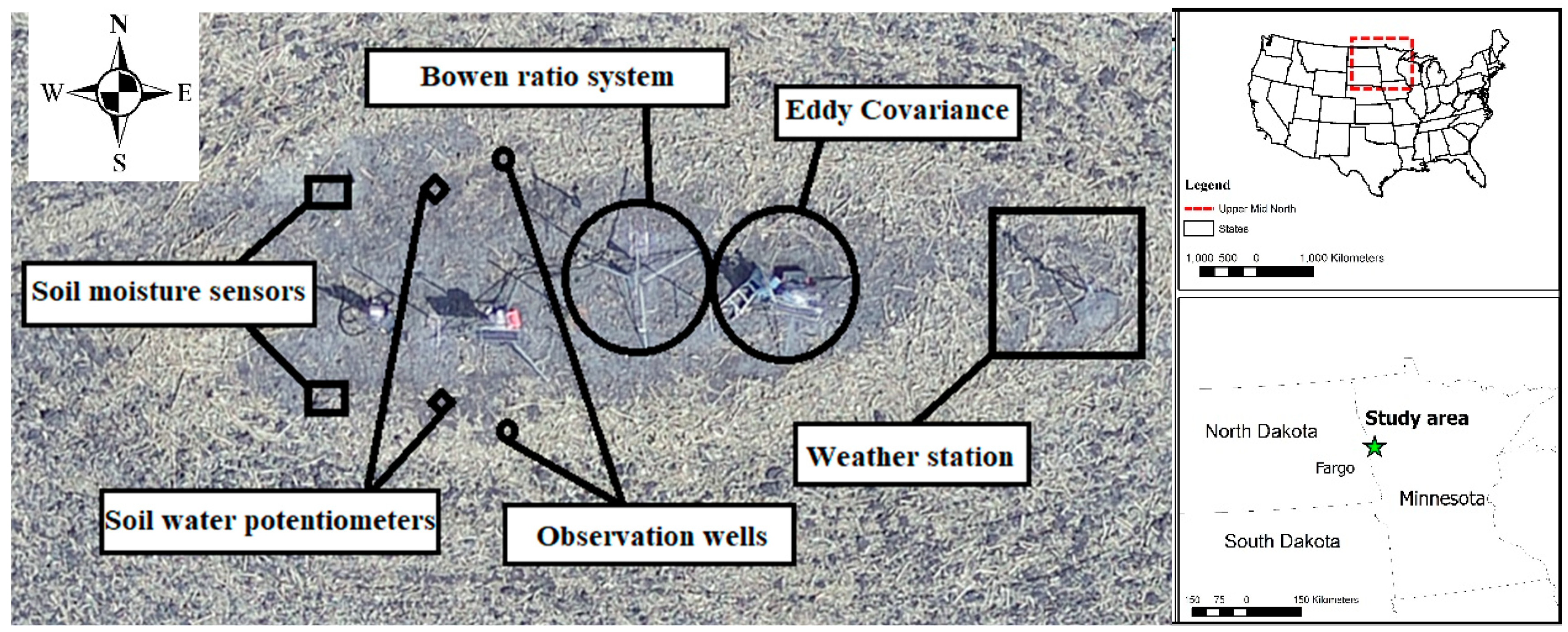
The study site is located in the Buffalo-Red River watershed in Clay County, west central Minnesota (46°59′20″ N, 96°41′06″ W) at an altitude of 271 m above sea level (Figure 1). The climate of the region is sub-humid, with a cold winter and a mild and humid summer. The location receives a mean annual precipitation between 533 and 635 mm, with 428 mm rainfall during the growing season in 2018.
The study site is on 54 ha field with less than 1% slope where a subsurface drainage system had been installed in 2011 [23]. On 14 May 2018 corn was planted in the east west direction with a 76.5 cm row spacing. Corn had fully emerged on 24 May and was harvested on 11 November. From 23 July through 27 July 2018, a small amount of water was subirrigated through the drain tile.
Soils in the field are predominantly classified as poorly drained with parts having a Bearden silt loam (50% of the total area), an Overly silty clay loam (27% of the area), and a Colvin silty clay loam (23% of the area), with an impermeable layer at about 3 m depth [23]. The soil properties for the different soil layers near the EC and BREB towers were measured by the cylindrical core method [24] by the end of the soil release curve measurement at saturation condition. The particle analysis was performed by the pipette method [25]. The results are shown in Table 1.
2.2. Evapotranspiration Measurement
2.2.1. Eddy Covariance
Details about the EC system, associated meteorological measurements, soil water and water table depth monitoring, and data processing were previously described by Niaghi et al. [23,26]. The EC was installed in the middle of the field with fetch over 150 m in all directions. Considering that the field is sufficiently flat and homogenous, the exchange fluxes are one-dimensional and can be calculated using covariance between vertical wind speed and the scalar of interest. H fluxes at the EC site were estimated directly using a CSAT3 sonic anemometer (Campbell Scientific, Inc., Logan, UT, USA). Due to the limitation on the tower height, the instruments were kept approximately 0.6 m above the canopy when the corn reached its maximum height. As a rule of thumb for agricultural weather stations, the EC system should be kept at least 1 m above the crop canopy to avoid any site aridity effects [27]. However, for a humid region with high wind speed conditions (>2 m/s) most of the time, the instrumentation height would have a minimal effect on the flux measurement [28]. Additionally, the analysis using the 10 Hz flux data revealed that the shapes of the spectral and co-spectral analysis were valid [23]. The CR3000 datalogger (Campbell Scientific, Inc., Logan, UT, USA) recorded signals from the EC system at a frequency of 10 Hz, which were corrected for wind speed rotation (based on double rotation and detrending by the block method), time lags (using maximum covariance approaches), spike effect (plausibility range within 5 standard deviations), and amplitude resolution (with range variation within 7 standard deviations) [23]. The corrected data were averaged over 30 min intervals for ET calculations. The soil heat flux (G) was measured with a pair of HFT3-L soil heat plates (REBS Soil Heat Flux Plate, Radiation and Energy Balance Systems, Inc., Bellevue, WA, USA). These sensors were installed at 8 cm depth and at 0.5 m distance between each other to reduce the spatial variability, and two soil thermocouples were placed at 2 and 6 cm above each of the soil heat flux plates. The measured G was corrected for soil heat storage by considering the soil water content. Finally, the residual method was used to close the energy balance for the EC system by assuming that the H was measured correctly. More details on the EC system and method were described in previous studies [23,29].
2.2.2. Bowen Ratio System
The BREB system was used to directly measure a vertical gradient of temperature and relative humidity. BREB included fan-aspirated housings mounted on a chain-driven automatic exchange mechanism (AEM, Radiation and Energy Balance Systems, Bellevue, WA, USA). The AEM switched the gradient measuring positions between the top and bottom every 15 minutes to reduce the effects of instrument offsets. Each arm of the AEM had a Vaisala T/RH probe inside an air-aspirated shield with 1 m separation between the arms to measure temperature and relative humidity at two heights. Furthermore, each probe included two calibrated thin film platinum resistance temperature sensors (PRTDs) (Vaisala Inc., Model #s HMP 35A and HMP 35D, Finland), one of them measuring the air temperature for a temperature gradient calculation, and the other measuring the air temperature of the humidity sensor cavity of the probe for a saturated vapor pressure calculation. To measure the net radiation (Rn), measurements from two REBS Q*7.1 net radiometers (Campbell Scientific, Inc., Logan, UT, USA) at 1 m above the crop canopy, with an adjustment by crop growth, were averaged, and the measured values were corrected for a wind speed effect [30]. For the G measurement and correction, 3 sets of soil moisture probes at a 0.5 m distance and 2.5 cm depth (REBS SMP-1), soil heat flow plates at 5 cm depth (REBS-HFT-3), and soil temperature probes integrated at 0 to 5 cm depth (STP-1) were used. G measured by the soil heat flux plates was corrected for heat storage above the plates and the moisture effect. A Met One barometric pressure sensor (Met One Instruments Inc., Grant Pass, OR, USA), (in enclosure), a Met One 020 C wind direction sensor 2 m above the crop canopy, and a Met One 010 C wind speed sensor 2 m above the crop canopy were used. For data collection and storage, a CR1000 data logger (Campbell Scientific, Inc., Logan, UT, USA), with AM16/32 multiplexer was used. To supply the required energy and charging the battery, a 65 watt solar panel model M1910 (Radiation and Energy Balance Systems, Bellevue, WA, USA) was used.
The Bowen ratio (β) was estimated from the vertical gradient of temperature (T1, T2) and vapor pressure (e1, e2) at two heights using the AEM with 1.2 m separation and a lower arm with a 1 m difference above the crop canopy. β can be calculated as follows [15]:
where P is atmospheric pressure (kPa), Cp is specific heat of dry air (KJ/kg·°C), T1 and T2 are measured temperatures at two heights above the crop canopy (°C), ε is the ratio between the molecular weights of water vapor and air (0.622), Lv is the latent heat of vaporization (KJ/kg), e1 and e2 are vapor pressures measured at two heights above the crop canopy (kPa), and Kh and Kw are the eddy diffusivities for heat and water vapor, respectively, assumed to be equal. H is estimated as the residual of the energy balance, and LE is estimated as follows:
When β approaches “−1”, the calculated fluxes approach infinity. This situation normally occurs in early mornings and late afternoons, when H changes its sign due to irrigation, precipitation, or low values of vapor pressure difference (close to the resolution limit of the sensor) during times of low available energy [15]. In practice, when β is close to “−1”, LE and H have their minimal values and can be considered negligible. To process and check the quality of the data, the screening criteria described by Perez et al. [15] and Ohmura [14] were used to exclude the time stamps whenever β approached “−1”. Perez et al. [15] showed that the range of excluded interval for β around −1 depends on the measured vapor pressure gradient in each period and the resolution of the sensors. Therefore, by considering the resolution of the temperature (0.06 °C) and vapor pressure sensors (0.01 kPa), the excluded range for β (−1±) is calculated as follows:
where δΔe and γδΔT are the resolution limits for the vapor pressure and temperature gradient, and γ is a psychrometric constant (p.Cp/ε.Lv). In the growing season, only 3.8% of the BREB were rejected during the early morning and evening time.
ET can then be estimated from the LE values measured by the EC and BREB systems using the following equation:
where ET is in mm/30 min, LE is latent heat flux (W/m2), Lv is latent heat of vaporization (kJ/kg), and 1800 corresponds to 30 min in seconds.
2.2.3. Soil Water Balance
Two observation wells (depth 2 m) were installed near the EC and BREB towers to continuously monitor water table fluctuation using on a half hourly basis. The soil moisture was measured using impedance dielectric sensors (Hydra Prob II, Stevens Water Monitoring System, Inc., Portland, OR, USA) that were placed as a pair on a tile and between tiles at 8 depths (0–5, 5, 15, 30, 45, 60, 75, and 90 cm) near the two towers; the average of each depth was used as a volumetric soil water content (SWC) of the layer. Due to a datalogger malfunction, the recorded soil moisture data were not available during the second part of June.
Due to the shallow water table depth and clayey soil of the study site, frequent capillary rise could increase the soil water content above the water table depth. Guderle and Hildebrandt [31] observed that the uncertainties of the soil water sensors on root water uptake and capillary rise differ considerably among different approaches (e.g., the multi-layer regression method obtained the best estimation for selected 33 days during a dry period under possible measurement uncertainties). Therefore, an independent measurement of soil water potential may help to improve the estimation of the water table contribution to ET. To measure the hydraulic gradient at the lower boundary of the soil profile (1 m), six soil potentiometers (TEROS 21, Meter, Pullman, WA, USA) were installed at a paired location, on a drain tile and between two drain tiles, at 30, 60, and 90 cm depths. The measured water potential was used along with the soil moisture sensors to calculate the contribution of the water table to capillary rise. The average of the measured soil water potential at the two locations was used for 30, 60, and 90 cm soil layers to calculate the hydraulic gradient.
To calculate the capillary rise amount, the averaged soil potential in kPa for each soil layer was converted to a head of water and summed with the difference between the water table and the soil layer depth. The soil surface was considered as a datum, and positions below that were considered as negative depth. Therefore, potential hydraulic gradients were calculated in soil layers between the water table and 90 cm depth, between 90 and 60 cm depth, and between 60 and 30 cm depth. With the information in Table 1 and the soil retention curves developed using the HYPROP and WP4 methods, Van Gunechtan–Maulem parameters were estimated [32]. Along with the measured soil water content in the 30, 60, and 90 cm-depth layers, the hydraulic conductivity and effective hydraulic conductivity for each soil layer were obtained:
where K(θ) is hydraulic conductivity (cm/day), ks is saturated hydraulic conductivity (obtained from web soil survey, 8.64 for 0–30 cm and 0.87 cm/day for 30–90 cm soil layers, respectively), θ, θr, and θs are soil moisture, residual soil moisture, and saturated soil moisture content of each soil layer (cm3/cm3), and n is a constant. Thus, using the 1-D Richards equation between the water table depth and different soil layers for each half-hour time step, the capillary rise can be calculated as follows:
For Darcy’s equation, q is the flux rate (cm/day), h is the soil matric potential in cm, is the fluctuation of soil water potential in the head of water between water table depth for each half-hour measurement timesteps and study layer (Δz), in cm of water.
To calculate ET by the SWB method and the change of water storage in the root zone (considered at 90 cm depth), the following equation was used:
where P is precipitation in mm, RO is surface runoff in mm, which was ignored due to the low rainfall, flat topography, and dense planting during the observation periods (Ops), Iw is applied irrigation in mm, DP is deep percolation (mm), which is assumed as zero when θ is less than the field capacity, q is ground water contribution as an upward flow (mm/day), and zr is root depth in mm, all referred to day i. Thus, the ET by the SWB method was calculated as:
To calculate ET using the SWB method, different time periods were considered to obtain the most reliable results [33]. ET by the SWB method was calculated using four different time approaches, including daily average of the 30 min soil moisture data, average soil moisture between midnight and 2:00, average soil moisture between midnight and 4:00, and average soil moisture at 4:00.
2.3. Available Energy Analysis
Net radiation is important for LE estimation using the BREB and EC systems, and the net radiation measured by different instruments can vary considerably. To avoid measurement errors, two Q7.1 net radiometer (REBS, Bellevue, WA, USA) used in the BREB and EC systems were compared to a CNR1 net radiometer (Kipp and Zonen, Delf, The Netherland), where showed a good agreement with no significant difference. In this study, the average net radiation from the two Q7.1 net radiometer was used. Similarly, the average G from the two systems was used in the analysis.
2.4. Comparison during Observation Periods
Days with missing data or rainfall events (>10 mm) were excluded in the comparison. From 14 May to 17 October, we recorded 20% and 24% of data by the EC and the BREB systems, respectively, due to system malfunction or lost power, which were excluded from the final analysis.
Imukova et al. [34] observed that the ideal conditions for applying the water balance method are periods with low rainfall and low or absent seepage. Therefore, to minimize the uncertainties in drainage and seepage calculations, dry periods that met the mentioned criteria were selected from the growing season, which led to 6 OPs from May through October. Figure 2 shows the climate pattern of the growing season including the selected observation periods.
After measuring H with the EC and BREB systems, the accuracy of the residual method was compared between the two systems for both the entire growing season and the selected OPs. The error of the BREB system was examined during the study period. The SWB was applied to each OP, and the obtained ET values with and without considering the capillary rise were compared with those measured by the EC and BREB systems.
3. Results
3.1. Residual Method
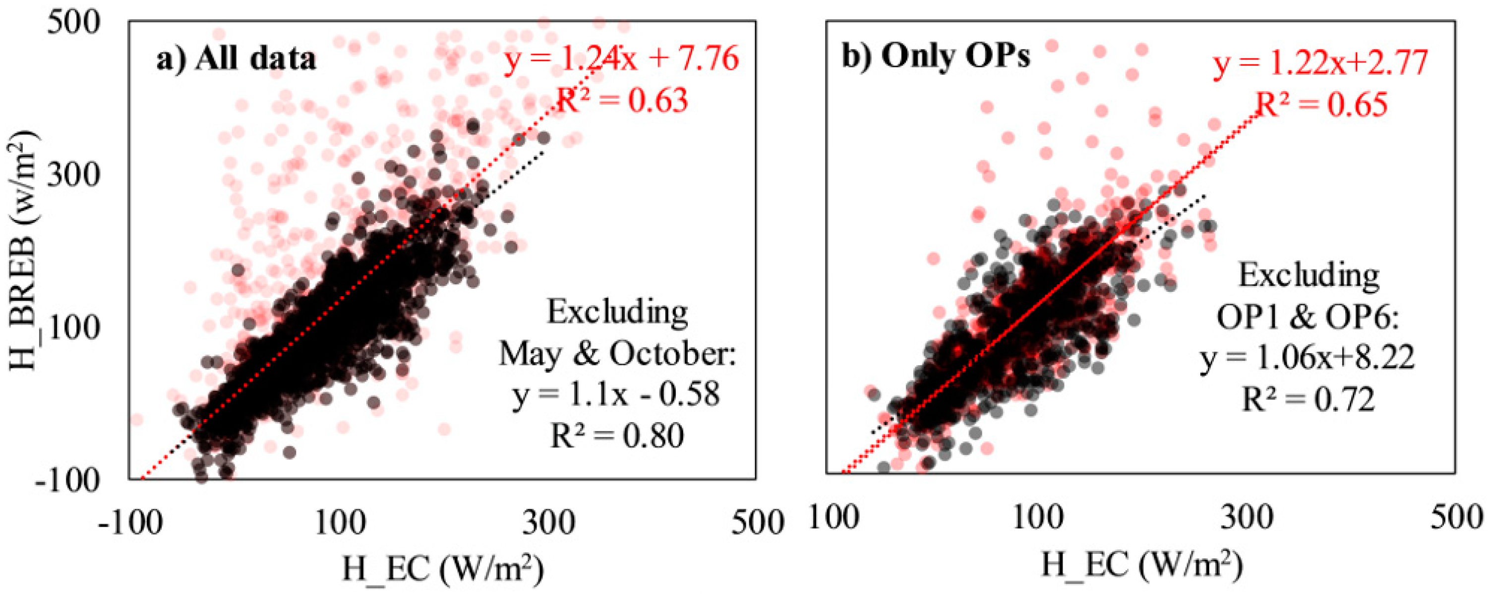
The validity and accuracy of the residual method for LE estimation using the EC system was evaluated with the BREB method as an independent method. Because the same available energy (Rn-G) was used for both systems, any difference in H could lead to an LE difference. Figure 3 illustrates the scatterplot for the measured H during 30 min between the BREB and the EC systems for the entire growing season and the OPs. The H values agreed well between the EC and the BREB systems when excluding the initial and harvesting months in May and October, respectively.
The statistical analysis of the data for the entire growing season and the OPs showed no significant differences (alpha = 0.01) between LE measured with the BREB system and LE estimated with the EC system. This indicated that the measured H by the EC system agreed well with the H determined by the independent BREB system, and thus, the accuracy of the residual method to estimate H was proved.
3.2. EC and BREB Comparison
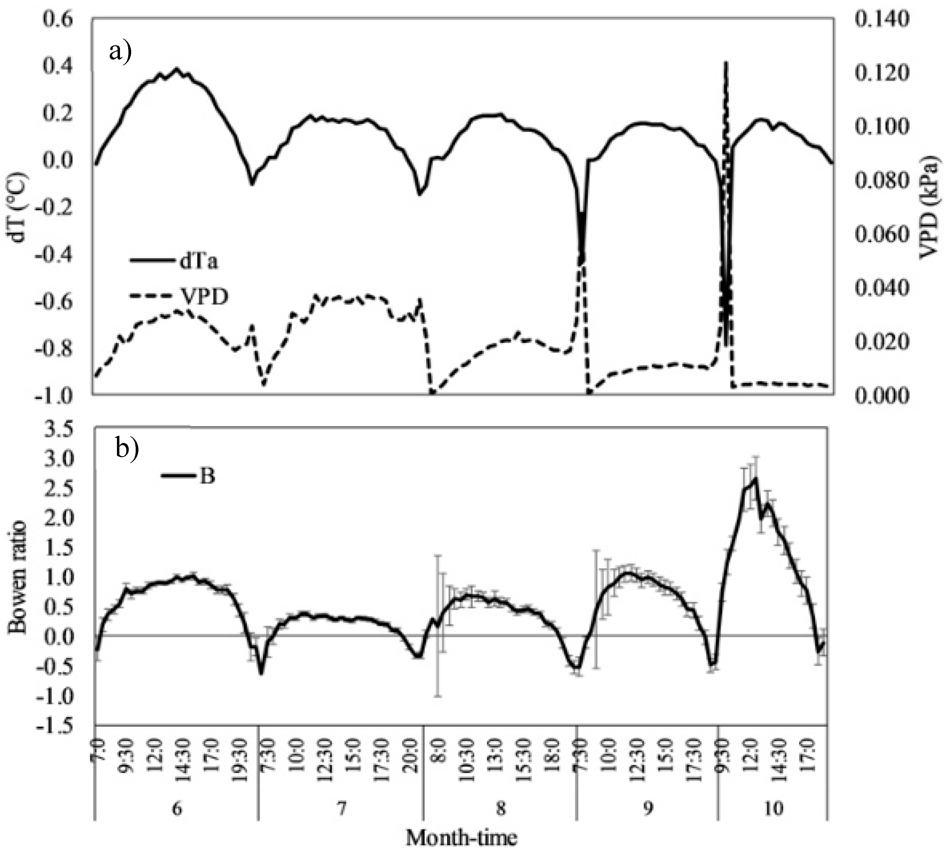
The diurnal fluctuation of temperature and the vapor pressure deficit (VPD) for the BREB measurements are shown in Figure 4. The highest measured error for β during the entire growing season was observed in August and September, when the crop reached its maximum height with a considerable stored energy within the crop canopy. The result agrees well with findings by Ohmura [14], indicating that the counter gradient flux during the early morning hours (6:00–8:00) and late evening (19:00–20:00) was a significant component of the energy balance when the H flux was toward the crop canopy. The standard deviation of measurement error fluctuated between 0.03 in July and 0.17 in September, with the highest estimated error between 7:00 and 8:30.
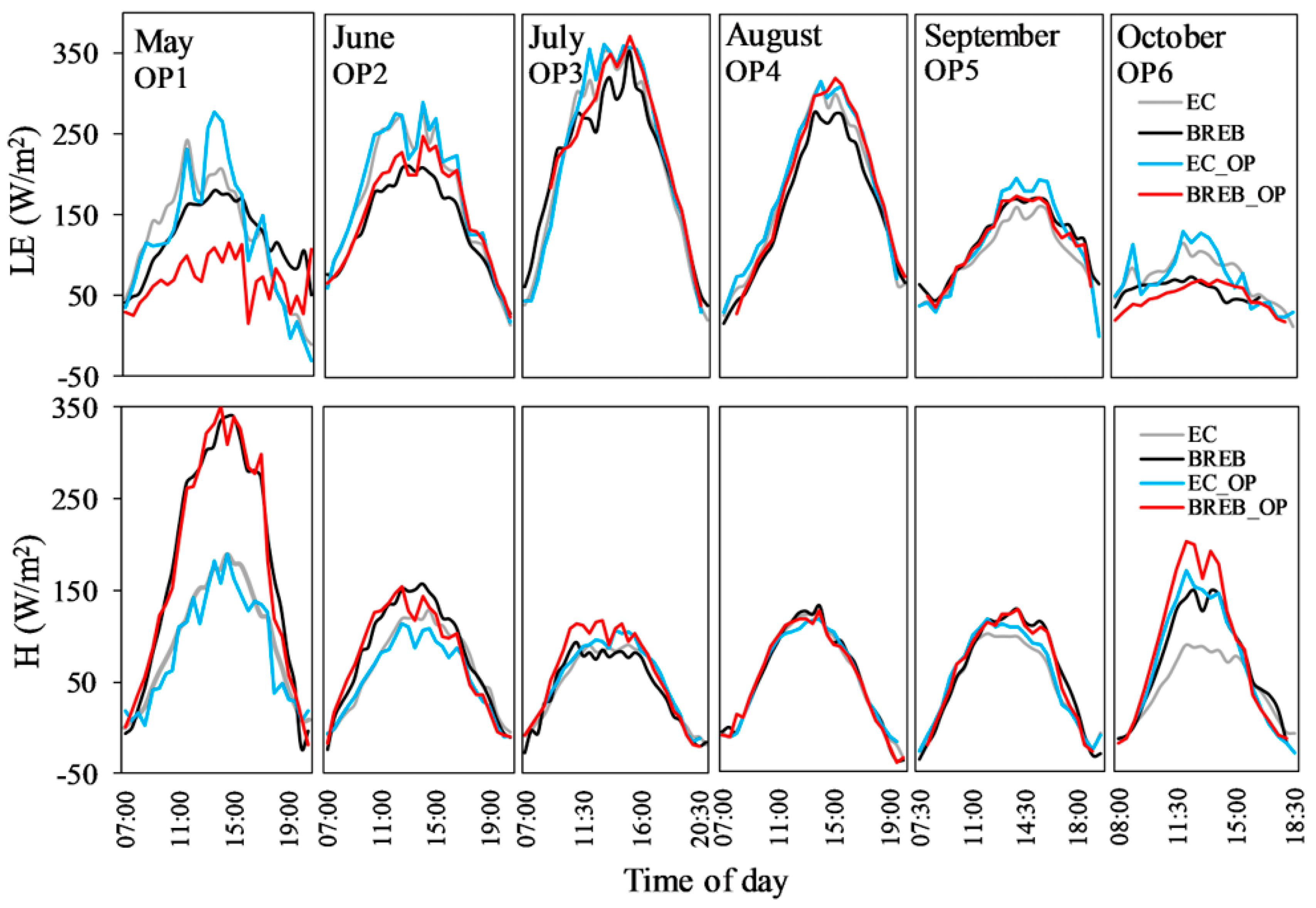
Diurnal variation of LE and H from the BREB and EC systems were examined by averaging the half-hour fluxes over each month of the growing season and during the OPs (Figure 5). Figure 5 indicated that the BREB and EC systems acted differently on partitioning the available energy during the early and late growth stages but agreed well for the mid-growth stage.
Table 2 shows the average climate condition and measured energy balance components for the OPs. Higher wind speed (U) and VPD were observed for OP1, in which measurements by the BREB and the EC systems showed the highest difference compared to those for other OPs. With crop growth and more ground coverage, the LE values increased for both systems.
3.3. Soil Water Balance and Capillary Rise
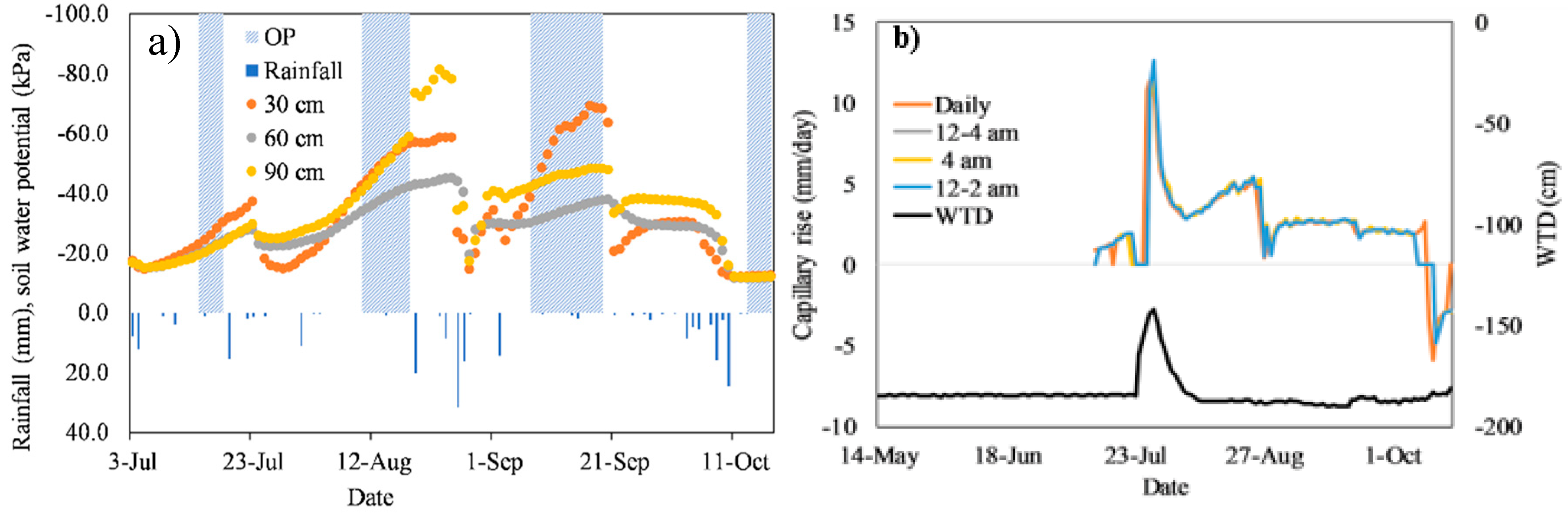
Even though some studies reported an 80% agreement on the ET measurements by the EC and SWB methods [11], uncertainties remained for others because the ET measurements were highly variable during periods with rainfall and rapid water movement within the soil profile. Figure 6 shows the average measured soil water potential and the calculated capillary rise along with the water table depth on a daily basis. Figure 6a illustrates the soil water potential in the soil profile during the dry periods from July to October. The water potential at the 90 cm depth had the lowest value (more negative), indicating a higher water movement from a deeper layer to the 90 cm layer. The water potential in the 60 cm layer was higher compared to that in the 90 cm depth, but there still was some water movement. The sudden decrease of soil water potential at the 30 cm depth during the mid-season after a rainfall event might have been caused by soil surface cracking and air entry into the sensor. Figure 6b shows that the water table depth was almost stable during the growing season, except in July when subirrigation was applied. The water table changed from below 185 cm on 22 July to 142 cm below the soil surface on 28 July. The estimated capillary rise from the soil water potential sensors clearly showed the effect of subirrigation, which increased the water potential in the soil profile and enhanced crop water uptake.
3.4. Estimated Evapotranspiration
Table 3 summarizes the calculated daily capillary rise, the average water table depth below the ground surface, and the average ET using the EC and BREB systems. The calculated average ET with and without considering the capillary rise effect for the different SWB approaches are also shown in Table 3. The ET values by the BREB method were compared with the ET values obtained from the EC and the SWB methods. ET determined by the EC method was, on average, about 10% higher than ET determined by the BREB method. For all OPs, the best agreement between ET values determined using the different SWB approaches and those determined by the BREB method was achieved for the soil water data for the 24:00–2:00 time period.
4. Discussion
The discrepancy between H values measured with the EC and BREB methods was probably due to a rapid corn growth during the early stage and the different in the instruments’ heights. As indicated by Niaghi et al. [23], the EC system was initially set up at 2.5 m in height and was later increased to about 3.2 m, whereas the BREB system was installed at 2 m in height (lower arm) and was increased up to 3.5 m in height (lower arm) in August. In addition, when the corn canopy did not cover the ground, advection and heat transfer from the surrounding area may have introduced an error in both systems. Schmid [35] reported that the footprint of the EC system is not fixed and varies in space due to wind direction and sensor height. The various wind speeds and directions in the study region during the early season may have led to a lack of accuracy for the early growing stages when the ground was not fully covered by crop [36]. When the corn grew and covered the ground, both the EC and the BREB systems had a similar footprint. Moreover, when compared to the H estimation by the BREB system, the underestimation of H by the EC system can be explained by the sonic anemometer frequency response, given atmospheric stability, canopy height, and wind speed. Dugas et al. [37] indicated that a correction of H due to the sonic anemometer frequency response would make H approximately 5% more negative. Another reason for H underestimation could be the short averaging period of the reference temperature time constant for sonic temperature correction [38]. On the other hand, for a stable condition when the ratio of heat and vapor diffusivity (β) was less than 1 (indication of BREB system failure) due to local advection, the measured β with the BREB system would be increased, and the H value would be more similar to the H value measured by EC.
Most research has shown that the sum of H and LE from EC instrumentation was always less than the available energy [29,34,39]. Thus, using the residual method, which accounts for the residual energy on LE, can lead to overestimation of LE (or ET) by the EC method with respect to the BREB method. However, LE overestimation by the EC method with respect to LE determined by the BREB method was 2.8%, −3.4%, and 4.9% for the development, tasseling, and reproductive stages, respectively. Therefore, in the current study, LE determined by the BREB method was compared with LE determined by the EC method, and the results revealed that the EC method is as accurate as the BREB method when crop is fully developed (fully covered ground) and when the residual method is applied to close the energy balance for the EC method. From OP2 to OP5, the available energy partitioning obtained by the EC and BREB systems showed a non-significant statistical difference. The lowest β value was observed for OP3, indicating a higher ratio of LE to H due to the higher crop water demand and more extensive ground coverage at the reproductive stage. The error and the standard deviation of the estimated β increased from OP5 to OP6 compared to the previous OPs. This error could be the result of stored heat within the crop canopy and exchange of that heat during early morning and late evening.
The BREB method has the advantage of obtaining ET independently without requiring information about the aerodynamic characteristics of the land surface [40]. However, due to the low available energy and large temporal Rn change around sunrise, the BREB method does not work properly, and the β value approaches “−1” at this time of the day. Thus, the equality assumption of the BREB method of turbulent exchange coefficient for heat and water vapor is not always met [41], and the recorded LE during this period needs to be either excluded or replaced using an interpolated value. Todd et al. [42] observed that 91% of half-hour daytime LE observations by the BREB system are valid. The comparison between ET values determined by a lysimeter and the BREB method showed that the greatest difference during the early growing season for alfalfa, while the ET values determined by the two systems were in agreement for the rest of the growing season [42].
Several approaches were attempted to quantify the water table contribution to ET. However, insufficient literature is available to address the effect of upward flux on the final SWB methodology and improve the accuracy of the SWB method. Using different approaches to calculate the soil water exchange on a day-to-day basis, we showed that the average nighttime soil moisture works better than the entire day average for ET calculation, due to the unstable conditions and uncertainties during daytime. In addition to the nighttime averaging method, considering the upward flux effect on the final ET calculation using the SWB method in areas with shallow water table can improve ET estimation, when compared to the in situ measurements of ET by the BREB and EC methods.
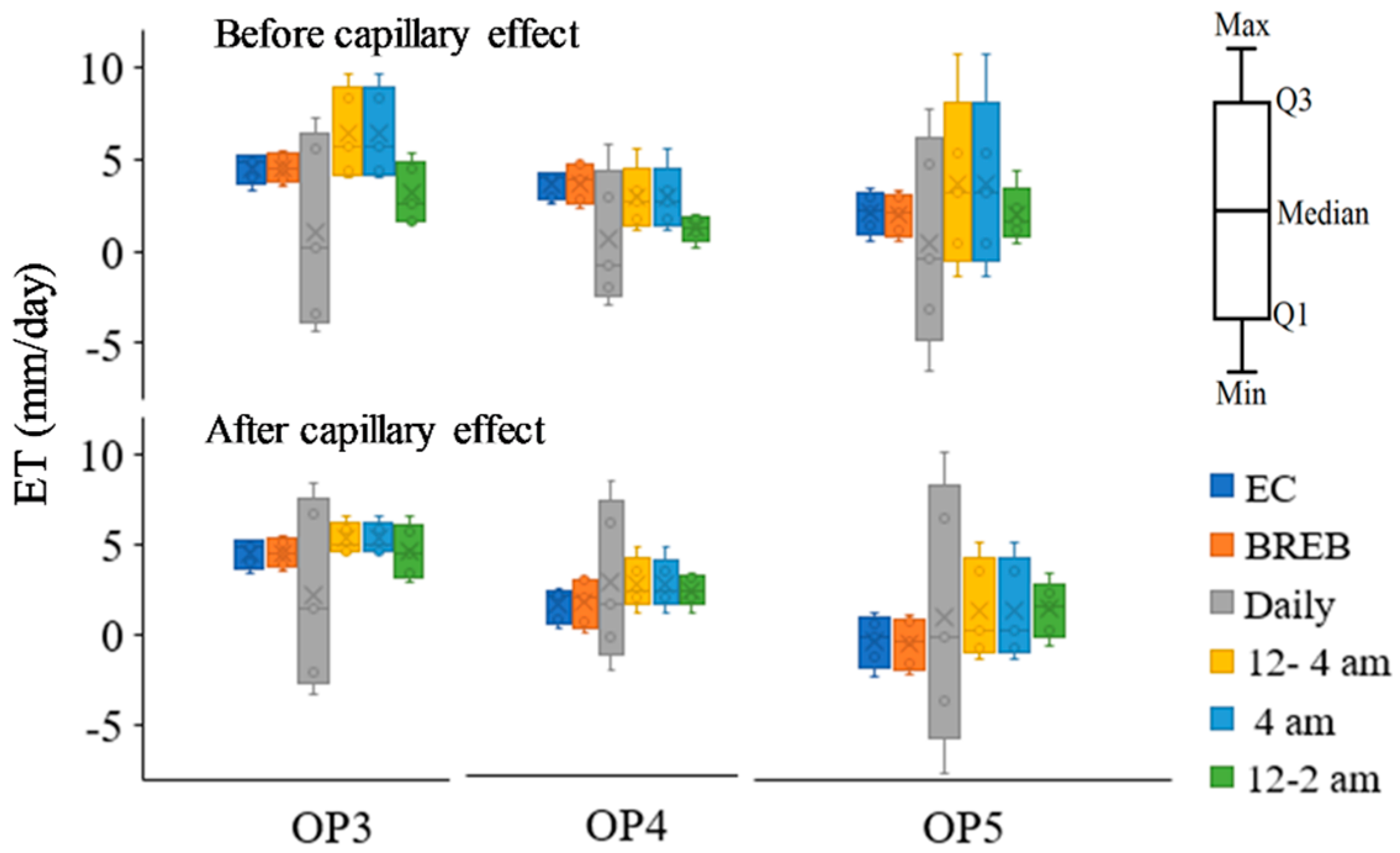
Figure 7 shows the boxplot comparison of ET determined at the different times with the SWB method with ET determined by the BREB and the EC method in OP3, OP4, and OP5. As shown in Figure 7, using the daily average soil moisture data to calculate the soil water exchange gave the worst ET result. Among the different approaches, using the average 24:00–2:00 soil water content for the daily ET calculation provided the best result in comparison with the ET values determined by the BREB and the EC methods and, statistically, showed no significant differences at a 95% confidence level.
Using the soil water exchange during the specific study period provides valuable information to calculate ET. This becomes more important during dry periods with high atmospheric demand [31,43]. The distinction between soil water exchange through the soil profile and water extraction by evaporation or transpiration is the major challenge of SWB application [31], since these fluxes occur concurrently during daytime [44]. Using the nighttime approach, this problem may be avoided. Li et al. [45] used a similar approach to derive the root water uptake pattern from soil moisture exchange using different time approaches. When using soil water content at nighttime, it can be inherently assumed that both nighttime evapotranspiration and hydraulic redistribution are negligible.
5. Conclusions
ET obtained from the EC system using the residual method to close the energy balance was evaluated with the BREB system for the entire growing season and for the selected OPs. The estimated LE by the EC system using the residual method showed a 29% overestimation compared to LE determined by the BREB system for the entire growing season. After excluding data in May and October, LE by the EC system was only 10% higher, indicating that the main difference between the two systems occurred during the early and later parts of the growing season. The overestimation of H by the EC method compared to the BREB method was about 24% for the total growing season and 22% for the OPs. These values decreased to 10% and 6% for the entire growing season and OPs, respectively, after excluding data in May and October. Overall, the comparison of H values measured by the EC and the BREB systems showed the best agreement when corn was fully developed (fully covered ground) and illustrated the advantages of using the residual method to close the energy balance in the EC method. The average diurnal LE and H showed good agreement between the EC and BREB methods during corn development, tasseling, and reproductive stages. In general, ET measured with the EC method was slightly higher than that determined by the BREB system. The current study shows that the residual method can be a reliable post-closure method with a higher accuracy when corn has covered the ground.
To compare and improve corn ET using the SWB method, four different time approaches (daily average, 24:00–2:00 average, 24:00–4:00 average, and 4:00 measure) were studied with and without considering the effect of capillary rise. Among the different time approaches, ET by the SWB method using the average soil water contents between 24:00 to 2:00 time period showed the best agreement with the ET measured by the BREB system. When considering the daily calculated hydraulic conductivity and upward flux in the soil water balance equation, ET accuracy was improved for all SWB approaches. For the 24:00–2:00 approach, the root-mean-square error (RMSE) and standard error values were calculated as 1.15 and 0.28, respectively. Non-significant differences (alpha = 0.05) were observed between the daily ET obtained with the 24:00–2:00 SWB approach and that obtained with the BREB system for OPs, indicating equal variance of the two methods. The shallow water table can significantly contribute to ET and therefore, improve the ET measurement by the SWB method when the soil water condition is a limiting factor. The application of the capillary rise to ET estimation using the SWB method during the mid to late crop stages can be as accurate as other expensive and complex ET methods, such as the EC and BREB methods.
Author Contributions
Conceptualization, methodology, software, validation, formal analysis, visualization, writing—original draft preparation, A.R.N.; and resources, writing—review and editing, supervision, funding acquisition, X.J.
Funding
This project is supported by USDA National Institute of Food and Agriculture project 2015-68007-23193, NASA ROSES Project NNX15AC47G, ND Water Resources Research Institute, ND Agricultural Experimental Station, and USDA Hatch project ND01482.
Acknowledgments
The authors would like to express their gratitude to Debra Baer for her assistance in reviewing the paper, Lin, and many other formal students for their valuable help in field work and data collection.
Conflicts of Interest
The authors declare no conflict of interest.
References
- Fisher, J.B.; Melton, F.; Middleton, E.; Hain, C.; Anderson, M.; Allen, R.; McCabe, M.F.; Hook, S.; Baldocchi, D.; Townsend, P.A.; et al. The future of evapotranspiration: Global requirements for ecosystem functioning, carbon and climate feedbacks, agricultural management, and water resources. Water Resour. Res. 2017, 53, 2618–2626. [Google Scholar] [CrossRef]
- Reyes-González, A.; Kjaersgaard, J.; Trooien, T.; Hay, C.; Ahiablame, L. Comparative Analysis of METRIC Model and Atmometer Methods for Estimating Actual Evapotranspiration. Int. J. Agron. 2017, 2017, 3632501. [Google Scholar] [CrossRef]
- Fidantemiz, Y.F.; Jia, X.; Daigh, A.L.M.; Hatterman-Valenti, H.; Steele, D.D.; Niaghi, A.R.; Simsek, H. Effect of water table depth on soybean water use, growth, and yield parameters. Water 2019, 11, 931. [Google Scholar] [CrossRef]
- Verstraeten, W.W.; Veroustraete, F.; Feyen, J. Assessment of evapotranspiration and soil moisture content across different scales of observation. Sensors 2008, 8, 70–117. [Google Scholar] [CrossRef] [PubMed]
- Zhang, B.; Kang, S.; Li, F.; Zhang, L. Comparison of three evapotranspiration models to Bowen ratio-energy balance method for a vineyard in an arid desert region of northwest China. Agric. For. Meteorol. 2008, 148, 1629–1640. [Google Scholar] [CrossRef]
- Dragoni, D.; Schmid, H.P.; Grimmond, C.S.B.; Loescher, H.W. Uncertainty of annual net ecosystem productivity estimated using eddy covariance flux measurements. J. Geophys. Res. Atmos. 2007, 112. [Google Scholar] [CrossRef]
- Amatya, D.M.; Irmak, S.; Gowda, P.; Sun, G.; Nettles, J.E.; Douglas-Mankin, K.R. Ecosystem evapotranspiration: Challenges in measurements, estimates, and modeling. Trans. ASABE 2016, 59, 555–560. [Google Scholar]
- Allen, R.G.; Pereira, L.S.; Howell, T.A.; Jensen, M.E. Evapotranspiration information reporting: I. Factors governing measurement accuracy. Agric. Water Manag. 2011, 98, 899–920. [Google Scholar] [CrossRef]
- Gebler, S.; Hendricks Franssen, H.-J.; Pütz, T.; Post, H.; Schmidt, M.; Vereecken, H. Actual evapotranspiration and precipitation measured by lysimeters: A comparison with eddy covariance and tipping bucket. Hydrol. Earth Syst. Sci. 2015, 19, 2145–2161. [Google Scholar] [CrossRef]
- Gong, J.; Shurpali, N.J.; Kellomäki, S.; Wang, K.; Zhang, C.; Salam, M.M.A.; Martikainen, P.J.; Imukova, K.; Ingwersen, J.; Hevart, M.; et al. Comparing different methods for determining forest evapotranspiration and its components at multiple temporal scales. Agric. For. Meteorol. 2016, 13, 595–605. [Google Scholar]
- Wilson, K.; Goldstein, A.; Falge, E.; Aubinet, M.; Baldocchi, D.; Berbigier, P.; Bernhofer, C.; Ceulemans, R.; Dolman, H.; Field, C.; et al. Energy balance closure at FLUXNET sites. Agric. For. Meteorol. 2002, 113, 223–243. [Google Scholar] [CrossRef]
- Consoli, S.; Vanella, D. Mapping crop evapotranspiration by integrating vegetation indices into a soil water balance model. Agric. Water Manag. 2014, 143, 71–81. [Google Scholar] [CrossRef]
- Irmak, S.; Kilic, A.; Chatterjee, S. On the Equality Assumption of Latent and Sensible Heat Energy Transfer Coefficients of the Bowen Ratio Theory for Evapotranspiration Estimations: Another Look at the Potential Causes of Inequalities. Climate 2014, 2, 181–205. [Google Scholar] [CrossRef]
- Ohmura, A. Objective criteria for rejecting data for Bowen ratio flux calculations. J. Appl. Meteorol. 1982, 21, 595–598. [Google Scholar] [CrossRef]
- Perez, P.J.; Castellvi, F.; Ibañez, M.; Rosell, J.I. Assessment of reliability of Bowen ratio method for partitioning fluxes. Agric. For. Meteorol. 1999, 97, 141–150. [Google Scholar] [CrossRef]
- Watanabe, K.; Yamamoto, T.; Yamada, T.; Sakuratani, T.; Nawata, E.; Noichana, C.; Sributta, A.; Higuchi, H. Changes in seasonal evapotranspiration, soil water content, and crop coefficients in sugarcane, cassava, and maize fields in Northeast Thailand. Agric. Water Manag. 2004, 67, 133–143. [Google Scholar] [CrossRef]
- Brotzge, J.A.; Crawford, K.C. Examination of the Surface Energy Budget: A Comparison of Eddy Correlation and Bowen Ratio Measurement Systems. J. Hydrometeorol. 2003, 4, 160–178. [Google Scholar] [CrossRef]
- Kolars, K.; Jia, X.; Steele, D.D.; Scherer, T.F. A soil water balance model for subsurface water management. Appl. Eng. Agric. 2019, 35, 633–646. [Google Scholar] [CrossRef]
- Ragab, R.A.; Amer, F. Estimating water table contribution to the water supply of maize. Agric. Water Manag. 1986, 11, 221–230. [Google Scholar] [CrossRef]
- Wallender, W.W.; Grimes, D.W.; Henderson, D.W.; Stromberg, L.K. Estimating the Contribution of a Perched Water Table to the Seasonal Evapotranspiration of Cotton. Agron. J. 1979, 71, 1056–1060. [Google Scholar] [CrossRef]
- Prathapar, S.A.; Robbins, C.W.; Meyer, W.S.; Jayawardane, N.S. Models for estimating capillary rise in a heavy clay soil with a saline shallow water table. Irrig. Sci. 1992, 13, 1–7. [Google Scholar] [CrossRef]
- Prathapar, S.A.; Meyer, W.S. Measurement and estimation of capillary upflow from watertables under maize on irrigated soils. Aust. J. Soil Res. 1993, 31, 119–130. [Google Scholar] [CrossRef]
- Niaghi, A.R.; Jia, X.; Steele, D.D.; Scherer, T.F. Drainage water management effects on energy flux partitioning, evapotranspiration, and crop coefficients of corn. Agric. Water Manag. 2019, 225, 105760. [Google Scholar] [CrossRef]
- Doran, J.W.; Jones, A.J.; Arshad, M.A.; Lowery, B.; Grossman, B. Physical Tests for Monitoring Soil Quality. In Methods for Assessing Soil Quality; SSSA Special Publication 49; Soils Science Society of Amercia: Madison, WI, USA, 1996. [Google Scholar]
- Gee, G.; Or, D. Methods of Soil Analysis; SSSA Book Series 5.4; Soils Science Society of Amercia: Madison, WI, USA, 2002. [Google Scholar]
- Niaghi, A.R.; Jia, X. Determination of Grass Evapotranspiration Rates and Crop Coefficients Using Eddy Covariance Method in Eastern North Dakota. In Proceedings of the World Environmental and Water Resources Congress, American Society of Civil Engineers, Reston, VA, USA, 21–25 May 2017; pp. 468–483. [Google Scholar]
- ASABE Standards. EP505: Measurement and Reporting Practices for Automatic Agricultural Weather Station; ASABE Standards: St. Joseph, MI, USA, 2004. [Google Scholar]
- Jia, X.; Dukes, M.D.; Jacobs, J.M.; Haley, M. Impact of weather station fetch distance on reference evapotranspiration calculation. In Proceedings of the Restoring Our Natural Habitat. In Proceedings of the 2007 World Environmental and Water Resources Congress, Tampa, FL, USA, 15–19 May 2007. [Google Scholar]
- Niaghi, A.R.; Jia, X.; Scherer, T.; Steele, D. Measurement of unirrigated turfgrass evapotranspiration rate in the red river valley. Vadose Zone J. 2019, 18, 1–37. [Google Scholar] [CrossRef]
- Campbell Scientific Inc. Q-7.1 Net Radiometer; Campbell Scientific Inc.: Logan, UT, USA, 1996; Volume 5. [Google Scholar]
- Guderle, M.; Hildebrandt, A. Using measured soil water contents to estimate evapotranspiration and root water uptake profiles—A comparative study. Hydrol. Earth Syst. Sci. 2015, 19, 409–425. [Google Scholar] [CrossRef]
- Roy, D.; Jia, X.; Steele, D.D.; Lin, D. Development and Comparison of Soil Water Release Curves for Three Soils in the Red River Valley. Soil Sci. Soc. Am. J. 2018, 82, 568–577. [Google Scholar] [CrossRef]
- Malek, E. Comparison of the Bowen ratio-energy balance and stability-corrected aerodynamic methods for measurement of evapotranspiration. Theor. Appl. Climatol. 1993, 48, 167–178. [Google Scholar] [CrossRef]
- Imukova, K.; Ingwersen, J.; Hevart, M.; Streck, T. Energy balance closure on a winter wheat stand: Comparing the eddy covariance technique with the soil water balance method. Biogeosciences 2016, 13, 63–75. [Google Scholar] [CrossRef]
- Schmid, H.P. Experimental design for flux measurements: Matching scales of observations and fluxes. Agric. For. Meteorol. 1997, 87, 179–200. [Google Scholar] [CrossRef]
- Grare, L.; Lenain, L.; Melville, W.K. The influence of wind direction on Campbell scientific CSAT3 and Gill R3-50 sonic anemometer measurements. J. Atmos. Ocean. Technol. 2016, 33, 2477–2497. [Google Scholar] [CrossRef]
- Dugas, W.A.; Fritschen, L.J.; Gay, L.W.; Held, A.A.; Matthias, A.D.; Reicosky, D.C.; Steduto, P.; Steiner, J.L. Bowen ratio, eddy correlation, and portable chamber measurements of sensible and latent heat flux over irrigated spring wheat. Agric. For. Meteorol. 1991, 56, 1–20. [Google Scholar] [CrossRef]
- Moore, C.J. Frequency response corrections for eddy correlation systems. Bound. Layer Meteorol. 1986, 37, 17–35. [Google Scholar] [CrossRef]
- Leuning, R.; van Gorsel, E.; Massman, W.J.; Isaac, P.R. Reflections on the surface energy imbalance problem. Agric. For. Meteorol. 2012, 156, 65–74. [Google Scholar] [CrossRef]
- Shi, T.T.; Guan, D.X.; Wu, J.B.; Wang, A.Z.; Jin, C.J.; Han, S.J. Comparison of methods for estimating evapotranspiration rate of dry forest canopy: Eddy covariance, Bowen ratio energy balance, and Penman-Monteith equation. J. Geophys. Res. Atmos. 2008, 113, 1–15. [Google Scholar] [CrossRef]
- Barr, A.G.; King, K.M.; Gillespie, T.J.; Den Hartog, G.; Neumann, H.H. A comparison of bowen ratio and eddy correlation sensible and latent heat flux measurements above deciduous forest. Bound. Layer Meteorol. 1994, 71, 21–41. [Google Scholar] [CrossRef]
- Todd, R.W.; Evett, S.R.; Howell, T.A. The Bowen ratio-energy balance method for estimating latent heat flux of irrigated alfalfa evaluated in a semi-arid, advective environment. Agric. For. Meteorol. 2000, 103, 335–348. [Google Scholar] [CrossRef]
- Hupet, F.; Vanclooster, M. Intraseasonal dynamics of soil moisture variability within a small agricultural maize cropped field. J. Hydrol. 2002, 261, 86–101. [Google Scholar] [CrossRef]
- Feddes, R.A.; Raats, P.A.C. Parameterizing the soil–water–plant root system. Wagening. Front. Ser. 2004, 6, 95–141. [Google Scholar]
- Li, Y.; Fuchs, M.; Cohen, S.; Cohen, Y.; Wallach, R. Water uptake profile response of corn to soil moisture depletion. Plant Cell Environ. 2002, 25, 491–500. [Google Scholar] [CrossRef]
Figure 1.
Aerial view of the instruments at the study site in Clay County, MN.

Figure 2.
(a) Average daily soil water content (SWC) and (b) average daily temperature, relative humidity, and rainfall amount during the 2018 growing season. Tan colored zones show the observation periods (OPs).
Figure 2.
(a) Average daily soil water content (SWC) and (b) average daily temperature, relative humidity, and rainfall amount during the 2018 growing season. Tan colored zones show the observation periods (OPs).

Figure 3.
Comparison of measured sensible heat flux (H) using the eddy covariance (EC) and Bowen ratio-energy balance (BREB) methods for the entire growing season (a) and the OPs (b). The right corner of the plots shows the fitting equations when excluding data in May and October for all data in (a), and OP1 and OP6 for Ops in (b).

Figure 4.
(a) Diurnal fluctuation of air temperature (dTa) and vapor pressure deficit (VPD) and (b) measured monthly average Bowen ratio (β) and calculated error for β on a diurnal basis.
Figure 4.
(a) Diurnal fluctuation of air temperature (dTa) and vapor pressure deficit (VPD) and (b) measured monthly average Bowen ratio (β) and calculated error for β on a diurnal basis.

Figure 5.
Average diurnal latent heat (LE) and sensible heat (H) flux using the EC and BREB systems for each month of the growing season and the OPs.
Figure 5.
Average diurnal latent heat (LE) and sensible heat (H) flux using the EC and BREB systems for each month of the growing season and the OPs.

Figure 6.
(a) Daily average soil water potential at three depths during the OPs and (b) daily average water table depth (WTD) and calculated capillary rise from a shallow water table.
Figure 6.
(a) Daily average soil water potential at three depths during the OPs and (b) daily average water table depth (WTD) and calculated capillary rise from a shallow water table.

Figure 7.
Boxplot of estimated crop ET using the SWB method with different approaches (daily average soil moisture: daily, 12–4 am average soil moisture: from 24:00 to 4:00, 4 am soil moisture: at 4:00, and 12–2 am average soil moisture: from 24:00 to 2:00), the BREB, and the EC methods without (before) capillary effect and with (after) capillary effect for July, August, and September OPs (OP3, OP4, and OP5).


Table 1.
Soil particle size in different soil layers.
| Layer | Sand | Silt | Clay |
|---|---|---|---|
| cm | Percent | ||
| 0–30 | 1.1 | 61.7 | 37.2 |
| 30–60 | 0.5 | 71.8 | 27.8 |
| 60–90 | 1.0 | 50.5 | 48.6 |
| 90–120 | 1.2 | 65.2 | 33.7 |
Table 2.
Summary of daily averages of climate variables and energy balance components for each of the selected OPs during the corn growing season in 2018. Air temperature = T, wind speed = U, vapor pressure deficit = VPD, Rn = net radiation, G = soil heat flux, H = sensible heat flux, LE = latent heat flux, and β = Bowen ratio.
| Observation | OP1 | OP2 | OP3 | OP4 | OP5 | OP6 |
|---|---|---|---|---|---|---|
| Period | 20–25 May | 20–28 June | 14–18 July | 10–18 August | 7–19 September | 14–17 October |
| Stage | Initial | Development | Reproductive | Tasseling | Maturity | Harvesting |
| Average climate data | ||||||
| T, °C | 23.0 (6.0) * | 25.1 (3.7) | 24.3 (4.0) | 24.8 (5.6) | 21.0 (5.9) | 3.4 (3.6) |
| U, m/s | 3.2 (1.9) | 1.9 (0.9) | 1.2 (0.5) | 1.2 (0.6) | 2.0 (0.9) | 2.4 (0.6) |
| VPD, kPa | 1.7 (1.0) | 1.4 (0.7) | 1.3 (0.6) | 1.3 (0.8) | 1.1 (0.8) | 0.3 (0.2) |
| Rainfall, mm | 0.8 | 0 | 1.3 | 1 | 3.3 | 0.2 |
| Energy, W/m2 | ||||||
| Rn | 246 (79) | 313 (28) | 390 (70) | 322 (48) | 233 (79) | 148 (75) |
| G | 35 (45) | 63 (15) | 57 (57) | 44 (12) | 31 (14) | 6 (9) |
| H_BREB | 158 (84) | 94 (14) | 87 (38) | 69 (45) | 82 (35) | 94 (65) |
| H_EC | 89 (23) | 66 (12) | 68 (22) | 77 (19) | 75 (27) | 70 (38) |
| LE_BREB | 63 (21) | 156 (18) | 246 (43) | 208 (56) | 120 (54) | 46 (15) |
| LE_EC | 126 (36) | 184 (23) | 230 (41) | 189 (33) | 124 (53) | 65 (39) |
| β _BREB | 2.3 (0.3) | 0.5 (0.1) | 0.3 (0.1) | 0.4 (0.4) | 0.7 (0.5) | 1.8 (1.1) |
| β_EC | 0.8 (0.3) | 0.4 (0.1) | 0.3 (0.2) | 0.4 (0.1) | 0.7 (0.3) | 1.3 (0.9) |
* All values inside the parentheses indicate standard deviation.
Table 3.
Summary of measured and estimated crop evapotranspiration (ET) using EC, BREB, and soil water balance (SWB) methods with different approaches for capillary rise calculation in different OPs.
Table 3.
Summary of measured and estimated crop evapotranspiration (ET) using EC, BREB, and soil water balance (SWB) methods with different approaches for capillary rise calculation in different OPs.
| Observation Period | OP1 | OP2 | OP3 | OP4 | OP5 | OP6 | |
|---|---|---|---|---|---|---|---|
| Date | 20–25 May | 20–28 June | 14–18 July | 10–18 August | 7–19 September | 14–17 October | |
| Stage | Initial | Development | Reproductive | Tasseling | Maturity | Harvesting | |
| Rainfall, mm | 0.8 | 0 | 1 | 1 | 3.3 | 0 | |
| Capillary rise, mm | - | - | 1.2 ± 0.2 | 4.1 ± 0.5 | 2.6 ± 0.1 | - | |
| Water table depth, cm | −184.6 | −184.5 | −184.4 | −187.4 | −189.4 | 183.6 | |
| Average ET, mm/day | |||||||
| ET reference | 5.2 ± 1.2 * | 5.2 ± 0.6 | 5.3 ± 0.8 | 4.5 ± 1.1 | 4.1 ± 1.6 | 1.8 ± 0.5 | |
| ET by EC | 2.5 ± 0.8 | 3.7 ± 0.5 | 4.6 ± 0.8 | 3.5 ± 0.6 | 2.1 ± 0.9 | 0.9 ± 0.6 | |
| Total | 15.3 (0.85) ** | 33.2 (0.89) | 22.9 (0.48) | 32.7 (0.50) | 27.4 (0.33) | 4.3 (0.31) | |
| ET by BREB | 1.9 ± 0.6 | 3.7 ± 0.6 | 4.7 ± 0.7 | 3.5 ± 0.9 | 2.1 ± 0.9 | 0.9± 0.3 | |
| Total | 11.1 | 28.8 | 22.6 | 33.1 | 26.1 | 3.7 | |
| SWB +non capillary effect | daily | 0 ± 2.7 | - | 1.5 ± 4.7 | 0.2 ± 2.9 | 0.2 ± 4.5 | 0 ± 3.1 |
| 24:00–4:00 | 1.3 ± 1.0 | - | 6.2 ± 2.2 | 2.6 ± 1.3 | 3.2 ± 3.4 | 1.6 ± 0.9 | |
| 4:00 | 1.6 ± 2.0 | - | 5.5 ± 2.2 | 2.6 ± 1.3 | 3.2 ± 3.4 | 1.1 ± 1.1 | |
| 24:00–2:00 | 0.6 ± 0.4 | - | 2.7 ± 1.6 | 1.2 ± 0.5 | 1.7 ± 1.0 | 0.7 ± 0.6 | |
| SWB with capillary effect | daily | 0 ± 2.7 | - | 2.1 ± 4.6 | 4.2 ± 2.8 | 2.8 ± 4.5 | 0 ± 3.1 |
| 24:00–4:00 | 1.3 ± 1.0 | - | 5.2 ± 0.8 | 4.3 ± 0.9 | 3.2 ± 1.7 | 1.6 ± 0.9 | |
| 4:00 | 1.6 ± 2.0 | - | 5.2 ± 0.8 | 4.3 ± 0.8 | 3.2 ± 1.7 | 1.1 ± 1.1 | |
| 24:00–2:00 | 0.6 ± 0.4 | - | 4.5 ± 1.3 | 4.1 ± 0.5 | 3.4 ± 1.0 | ± 0.6 | |
* Standard deviation; ** value inside the parentheses indicate root-mean-square error.
© 2019 by the authors. Licensee MDPI, Basel, Switzerland. This article is an open access article distributed under the terms and conditions of the Creative Commons Attribution (CC BY) license (http://creativecommons.org/licenses/by/4.0/).
Share and Cite
MDPI and ACS Style
Rashid Niaghi, A.; Jia, X. New Approach to Improve the Soil Water Balance Method for Evapotranspiration Estimation. Water 2019, 11, 2478. https://doi.org/10.3390/w11122478
AMA Style
Rashid Niaghi A, Jia X. New Approach to Improve the Soil Water Balance Method for Evapotranspiration Estimation. Water. 2019; 11(12):2478. https://doi.org/10.3390/w11122478
Chicago/Turabian StyleRashid Niaghi, Ali, and Xinhua Jia. 2019. "New Approach to Improve the Soil Water Balance Method for Evapotranspiration Estimation" Water 11, no. 12: 2478. https://doi.org/10.3390/w11122478
Note that from the first issue of 2016, this journal uses article numbers instead of page numbers. See further details here.