Article

Jointly Modeling Drought Characteristics with Smoothed Regionalized SPI Series for a Small Island

by
Luis Angel Espinosa
1,2,*,
Maria Manuela Portela
1,
João Dehon Pontes Filho
3,
Ticiana Marinho de Carvalho Studart
3,
João Filipe Santos
4 and
Rui Rodrigues
2
1
Instituto Superior Técnico (IST), Civil Engineering Research and Innovation for Sustainability (CERIS); Universidade de Lisboa, Instituto Superior Tecnico (IST), Department of Civil Engineering, Architecture and Georesources (DECivil), Av. Rovisco Pais, 1, 1040-001 Lisbon, Portugal
2
National Laboratory for Civil Engineering (LNEC), Lisbon 1700-066, Portugal
3
Hydraulic and Environmental Engineering Department (DEHA), Federal University of Ceará, Fortaleza 60020-181, Brazil
4
Department of Engineering, Polytechnic Institute of Beja, 7800-309 Beja, Portugal
*
Author to whom correspondence should be addressed.
Water 2019, 11(12), 2489; https://doi.org/10.3390/w11122489
Submission received: 22 October 2019 / Revised: 20 November 2019 / Accepted: 22 November 2019 / Published: 26 November 2019
(This article belongs to the Special Issue Management of Hydrological Extremes: Floods and Droughts)

Abstract

:
The paper refers to a study on droughts in a small Portuguese Atlantic island, namely Madeira. The study aimed at addressing the problem of dependent drought events and at developing a copula-based bivariate cumulative distribution function for coupling drought duration and magnitude. The droughts were identified based on the Standardized Precipitation Index (SPI) computed at three and six-month timescales at 41 rain gauges distributed over the island and with rainfall data from January 1937 to December 2016. To remove the spurious and short duration-dependent droughts a moving average filter (MA) was used. The run theory was applied to the smoothed SPI series to extract the drought duration, magnitude, and interarrival time for each drought category. The smoothed series were also used to identify homogeneous regions based on principal components analysis (PCA). The study showed that MA is necessary for an improved probabilistic interpretation of drought analysis in Madeira. It also showed that despite the small area of the island, three distinct regions with different drought temporal patterns can be identified. The copulas approach proved that the return period of droughts events can differ significantly depending on the way the relationship between drought duration and magnitude is accounted for.

1. Introduction

Droughts, perceived as prolonged and regionally extensive occurrences of below average natural water availability, are among the most destructive hazards and can arise virtually everywhere on the planet [1]. In island environments, where freshwater is often a limiting factor and people strongly rely on precipitation to refill the surface and underground water reservoirs and to support activities, such as rain-fed agriculture, droughts have frequently led to water insecurity—ranging from chronic water scarcity, lack of access to safe drinking water and sanitation services, to hydrological uncertainty [2,3,4]. As stated by the Intergovernmental Panel on Climate Change, IPCC, in its periodical assessment reports [5,6,7], compared to continental areas, islands are specifically more vulnerable to natural hazards due to their lower adaptive capacity, and are more often affected by extreme hydrological events (e.g., floods and droughts) and climate change, especially the so-called small islands with areas between 100 km 2 and 5000 km 2 [8]. Although small islands are not a homogeneous group, they share many common features that distinguish them from larger islands [9], which make more challenging their adaptation to the projected climate change risks—such as the increase in the probability of drought and rainfall deficits [10].
The pronounced hydrological temporal but also spatial variability in some of the small islands makes drought complex to analyze and simultaneously a poorly understood extreme hydrological events (e.g., compared to floods) [1]. Examples are Madeira with a very pronounced wet season and with notable differences in rainfall between northern and southern slopes; the nearby Porto Santo Island, with some signs of aridity and relatively low rainfall concentrated in a few days [11]; the Azores archipelago with very wet high regions and drier coastal areas [12]; and the Canary Islands, located in a dry belt with very low rainfall near the coast, especially in the flat islands [8]. These particular features have contributed to the absence of comprehensive drought assessment methods for small islands.
From a hydrological perspective, droughts are mainly characterized into three major types, with their own specific spatiotemporal characteristics [13], according to their duration and type of freshwater reservoir they affect: meteorological, agricultural, and hydrological droughts [14,15,16]. Meteorological droughts are characterized by a prolonged deficit of rainfall from its long-term average. Triggered by longer rainfall deficits, agricultural droughts are characterized by reduced soil moisture. Hydrological droughts are related to the impacts of persistent shortage of rainfall on lakes and reservoirs, rivers, surface water, and groundwater. Droughts can develop from over short periods (a few months) to longer periods (seasons, years, or even decades) [15,17].
The monitoring of drought employs widely used drought indices, such as the Palmer Drought Severity Index (PDSI) [18,19], the Standardized Precipitation Evapotranspiration Index (SPEI) [20,21], or the Standardized Precipitation Index (SPI) [22]. The PDSI uses precipitation and temperature data in a water balance model to compare meteorological and hydrological droughts across space and time, the SPEI considers precipitation and potential evapotranspiration, whereas the SPI only uses precipitation as state variable. Different authors have recommended that droughts should be studied within a regional context [17], because the results of individual case studies may not be comparable [23]. To make the drought analyses results comparable, regardless of the studied region, the drought indexes should be standardized [14] which is precisely one of the most important characteristics of the Standardized Precipitation Index. The SPI is likely to be the most frequently used drought indicator worldwide, because it is applicable in all climate regimes [14,24,25,26].
At given location, the SPI quantifies the observed rainfall as a standardized departure from a selected probability distribution function that models the raw rainfall data for the timescale of interest, from 1 to 48-month or longer (1, 3, 6, 9, and 12-month are the most common timescales [27]). The rainfall data are fitted to a probability distribution function, which is then transformed into a normal distribution so that the mean SPI for the location and desired timescale is zero [22]. Negative SPI values represent rainfall deficit, whereas positive SPI values indicate rainfall surplus.
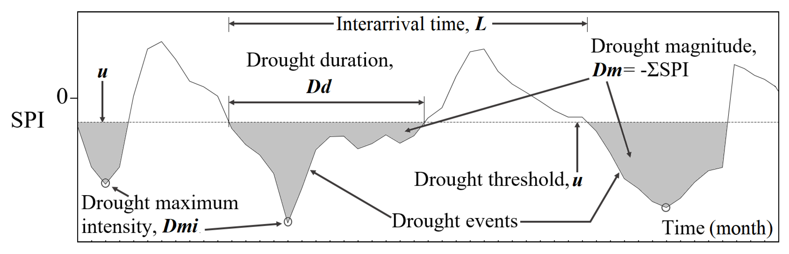
By applying the run theory [28] to the SPI series at a given timescale, the following characteristics of the droughts can be determined (Figure 1): drought duration ( D d ), during which the SPI is continuously below an adopted critical level or threshold (u); magnitude ( D m ) indicating the cumulative absolute deficit due to a drought event below the threshold; drought maximum intensity ( D m i ) indicating the minimum value of the drought index below the critical level, and interarrival time (L), which is the time range between the initiation of two consequent drought events.
However, drought characterization based on SPI requires particular attention, due to the possible presence of minor droughts and of mutually dependent droughts [30,31]. In fact, it is possible that a long SPI run below the threshold u turns out to be split into several shorter events due to the occurrence of sporadic and anomalous rainfalls [32] either for very short periods and with little hydrological importance, or for longer periods but unable to counterbalance the rainfall deficit. These smaller drought events cannot be considered mutually independent, and it is advisable to group them into a single large event to capture the true severity of the longer drought they portrait [30]. Filtering techniques can be applied for this purpose [33].
Another specific feature of the droughts is that although they are regional phenomena, the data required to characterize them are measurements acquired at discrete networks. Therefore, special clustering techniques need to be applied to enable a regional characterization based on pointwise data. Multivariate and geostatistical techniques are commonly used to analyze the spatial and temporal variability of climate variables—such as rainfall, temperature, and air relative humidity [34]. Principal components analysis (PCA) is a multivariate technique that has been relevant in these types of analyses, especially in climate regionalization [35,36,37,38]. It allows a field to be decomposed into spatial-temporal terms, such as in the analysis of the spatial and temporal variability of droughts characterized based on the SPI [25,26,39,40].
The last challenge when addressing the droughts relates to the capability of the models to describe the dependency among their different characteristics, which, as in many other hydrological phenomena, are presumably highly correlated and should be addressed from a multivariate perspective [41]. However, droughts have been traditionally studied in a univariate context [42], mostly aiming at recognizing their occurrences. Since a univariate approach ignores the dependence structure among the drought characteristics, it may result in a poorer representation of the phenomenon. The analysis of the association among those characteristics based on multivariate approaches although relevant, is still an insufficiently studied issue, namely in small islands.
In the scope briefly mentioned, this paper aims at presenting a pioneering study, particularly in its application to a small island, on drought characterization. For that purpose, Madeira (741 km 2 ) was selected as case study and the SPI at different timescales was computed based on 80 years of the monthly rainfalls at a large set of rain gauges distributed over the island. The mutually dependent droughts were assessed based on a digital filter, namely the moving average, MA, with different running lengths. By applying principal component analysis, PCA, to the original unfiltered SPI series, but also to the smoothed SPI series given by the MA, homogeneous regions were identified regarding the temporal pattern of the droughts. For each region, representative unsmoothed and smoothed regionalized SPI series were obtained and compared aiming at understanding the effect of the MA and at identifying the running length that should be adopted. Bivariate copulas were then applied to model the dependency structure between some of the drought characteristics extracted from the regionalized smoothed SPI series, namely drought duration, D d , and drought magnitude, D m . Finally, different return periods (univariate, bivariate and conditional) were assigned to the drought events.
The study provides a continuous and comprehensive temporal, but also spatial, characterization of the droughts in Madeira enabling an understanding of the susceptibility of the different regions to the phenomenon, as well as how it has changed along time.

2. Study Region and Data

Madeira is a volcanic island located in the North Atlantic Ocean with an area of 741 km 2 , a length of 57 km and a maximum width of 22 km. Centered at 32 44.34 N and 16 57.91 W, approximately 600 km northwest of the Western African coast, Madeira has a steep topography consisting of an enormous central E-W oriented mountainous system (Pico Ruivo, the highest peak with 1862 m.a.s.l.; Pico do Areeiro, in the island’s eastern part with 1818 m.a.s.l.; and Paúl da Serra region above 1400 m.a.s.l. on the west) which divides the island mainly into north and south from an orographical perspective. According to the Koppen’s classification [43], the climate is predominantly temperate with dry and warm to hot summers as approaching the coastal zones of Madeira.
Due to the strong topography influence, the rainfall falls predominantly in the north facing slope because of the prevailing N-E trade winds [11]. The rainfall regime, which is remarkably variable between the northern and southern slopes, is not only affected by the local circulation, but also by synoptic systems which are typical in mid-latitudes, such as fronts and extratropical cyclones, and the Azores Anticyclone in the summer season [44]. Rainfall in Madeira is concentrated in the period from October to mid-April, while in summer (from June to August) the rainfalls are very low [
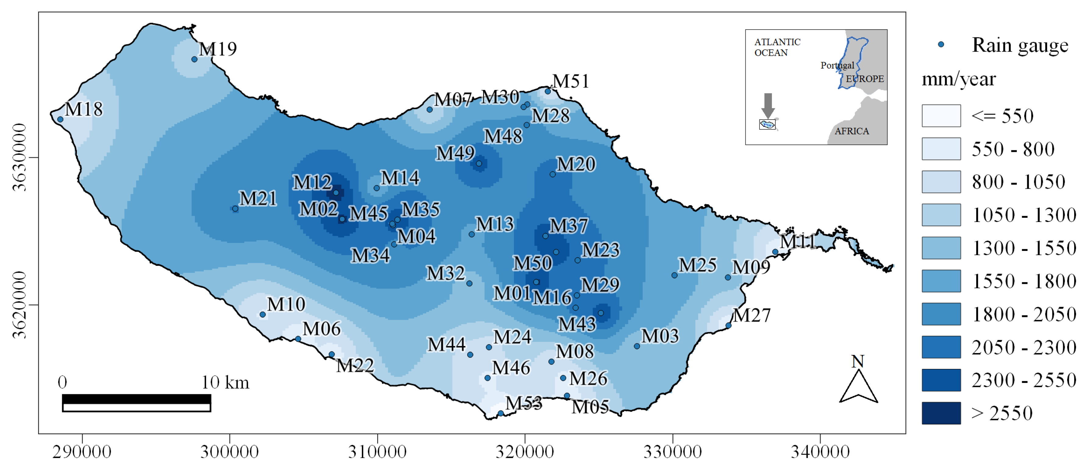
43]. The average annual rainfall in Madeira presents a very uneven distribution—Figure 2 and Table 1. The highest average annual values, exceeding 2200.0 mm, are observed in the northern slope and especially in the central highland region of the island (e.g., the rain gauges of M01 with 2592.2 mm, and M02 in the Paúl da Serra region with 2605.7 mm), which is the critical one for the island’s water security because it is where most of the natural groundwater recharge areas are located [45,46]. The smallest rainfalls, less than 650.0 mm, occur in the lowland areas of the southern slope (e.g., the rain gauge of M05 in the city of Funchal with only 608.4 mm).
The drought characterization in Madeira used the daily rainfalls, from January 1937 to December 2016 (80 years), at the 41 rain gauges of Figure 2 and Table 1. The records were provided by the Portuguese Institute for the Ocean and Atmosphere (IPMA), which has high data quality standards and is one of the main sources of Portuguese hydrometeorological data. The series had a few missing values that were filled in using a gap-filling procedure tested for Madeira, namely the Multiple Imputation by Chained Equations (MICE) [47,48]. The monthly and annual rainfall series were obtained from the complete daily series.

3. Methods

3.1. Standardized Precipitation Index (SPI) Calculation and Drought Recognition

As previously mentioned, the drought characterization used the SPI, developed by McKee et al. [22], and described in detail by Edwards and McKee [49]. Such index measures the rainfall anomalies at a given location, based on the comparison of the rainfall for a timescale of interest, with the average rainfall in the same period. The historic records are fitted to a probability distribution, which is then transformed into a normal distribution such that the mean SPI value for that location and timescale is zero. The Pearson Type III distribution with parameters given by the L-moments was applied to describe both the monthly rainfalls and the cumulative rainfalls at Madeira [26,47].
The drought events were assessed based on the SPI computed at 3 (SPI3) and 6 (SPI6) months for the period of 80 years (960 months of rainfall data) and for the 41 selected rain gauges. These two timescales are usually related to meteorological and agricultural droughts [50], and, the latter, also to early signs of streamflow shortfalls [27]. Such sustained shortfalls are very important for the management of water resources in Madeira due to its high dependence on rainfall for groundwater recharge—which is the main source of freshwater on the island [46,47]. The drought categories for SPI were those proposed by Agnew [51], presented in Table 2. According to this classification, there is a drought whenever the SPI falls below the threshold u < 0.84 . Furthermore, the droughts were characterized based on run theory as depicted in Figure 1. It is noteworthy that drought duration ( D d ) and magnitude ( D m ) are necessarily mutually dependent, because the longer D d is, the higher D m should be.

3.2. Moving Average Filter (MA)

Relatively few studies have addressed the run theory applied to the recognition of the drought characteristics (Figure 1) to cope with the possible dependence of the periods under drought conditions. Van Loon et al. [16], Fleig et al. [31], Tallaksen et al. [52] have applied moving average (MA), with different running lengths and at different SPI timescales, to smooth out short-term fluctuations and highlight possible longer drought events. Similar procedures have been carried out by López-Moreno et al. [30], although applied to drought analysis based on streamflow series, Zelenhasić and Salvai [53], Byzedi and Saghafian [54], Li et al. [55], Shin et al. [56]. However, criteria about the running length to adopt, also taking into account the different timescales of SPI, are missing.
The moving average (MA) is the most common filter in digital signal processing, mainly because it is the easiest to understand and use [33]. The MA is a convolution using a very simple filter kernel. This makes it the premier filter for encoded signals in the time domain in which samples are usually created by sampling at regular intervals of time containing information that is interpretable without reference to any other sample [57]. In the present paper, the MA operates by averaging several points from the input signal symmetrically chosen around each point in the output signal, according to:
y i = 1 M j = ( M 1 ) / 2 ( M 1 ) / 2 x i + j
where x i is the input signal, y i is the output signal, and M is the number of points in the average (running length). For M = 1 , the output coincides with the original or unsmoothed series.
For the smoothing of SPI3 and SPI6 at the adopted 41 rain gauges, Equation (1) was applied aiming at reducing the random noise, i.e., the spurious short droughts and drought interruptions, while maintaining a sharp step response (e.g., D m , D m i ). Different M were tested and assessed for each SPI timescale, namely for SPI3, 2 and 3, and for SPI6, 3 and 5. The SPI output series for M equal to 1, have obviously the same values as the input series and were also analyzed for both timescales (unsmoothed series). Symmetrical averaging usually requires that M be an odd number. However, for the case of SPI3, because only two values could be adopted for M, they were both tested, despite one being an even number. It is acknowledged that the higher M, the greater the noise reduction, but also the greater the possibility that the signal would be distorted by the smoothing operation. A key issue in SPI series smoothing is the choice of M. In the Madeira case study, the selection of its value for each timescale was assessed based on the regionalized SPI series derived from the unsmoothed and smoothed SPI series at the 41 rain for different values of M, as discussed in Section 4.1.

3.3. Regionalized SPI Series Based on Principal Components Analysis (PCA)

Principal components analysis is a statistical procedure that transforms several (possibly) correlated variables into a (smaller) number of uncorrelated variables called principal components (PC) [58]. When applied to the SPI values from a set of rain gauges, it allows their regrouping and consequently, the delimitation of climatic regions in relation to synoptic situations, i.e., a regionalized SPI series—such as the three distinct areas with coherent climatic variability identified by Bonaccorso et al. [59] in Sicily from 1926 to 1996, the three homogeneous regions adopted for the drought characterization in mainland Portugal (which is approximately 120 times the size of Madeira) Santos et al. [29], or the two climatic sub-regions in the western Iran by Raziei et al. [60], all of them based on the SPI field. In the case of Madeira, the PCA was applied to the unsmoothed and smoothed (with different M) SPI time series at the timescales of 3 and 6 months.
The PCA consists of computing the covariance matrix of the SPI series with the corresponding eigenvalues ( λ ) and eigenvectors (v). The main applications of the PCA, specifically the principal factor analysis (PFA), are: (1) to reduce the number of variables; (2) to detect structures in the relationship between variables; (3) to reduce the system’s information entropy, i.e., the information not directly available about a system due to the uncertainty or randomness of data flow [61,62]; and (4) to combine correlated variables into factors [63]. As for Madeira, the variables are the SPI series at the rain gauges and the factors, the regionalized SPI. Henceforth, the term factor analysis will be used generically to encompass both PCA and PFA.
The determination of the number of components or factors to retain was based on the Kaiser’s rule [63], according to which the factors whose eigenvalues are greater than 1 must be retained. The spatial patterns of the eigenvectors (factor loadings) represent the correlation between the original data and the corresponding factor time series. More localized patterns are obtained by applying the Varimax rotation technique to selected factor loadings [64]. The projection of the SPI fields onto the orthonormal eigenfunctions provides the factor score time series [65]. Factor scores are estimates of the actual values of individual cases (observations). For instance, the estimated factor score (regionalized SPI) on factor j for observation, or month, i, F j i , can be represented as follows:
F j i = w j 1 z i 1 + w j 2 z i 2 + + w j k z i k
where w j is the regression weight, multidimensional value referred to as factor score coefficient; and z i is the variable, i.e., the SPI series at a single rain gauge. For any single common factor, an infinite number of sets of scores can be derived that would be consistent with the same factor loadings [66]. The factor scores are particularly useful to perform further regional analyses that have been identified in the factor analysis, such as fitting drought characteristics with copulas, as will be mentioned in the next subsections.

3.4. Univariate Analysis of Drought Duration and Magnitude; Selection of Probability Distribution Functions

The univariate analysis of drought duration, D d , and magnitude, D m , has not yet established a consensus on the marginal distribution to be used. Shiau [42] suggested the use of Exponential and Gamma distributions to model separately D d and D m , respectively. The advisable practice, however, is to test different families to achieve the best-fitted model for each region and drought characteristic [67,68]. Thus, in this study, Exponential, Gamma, Logistic, Log-Normal, Normal, and Weibull were inspected—based on the most relevant factor scores for the smoothed regionalized SPI3 and SPI6 series—to determine the most suitable distribution function for drought duration and magnitude values. The Akaike Information Criterion (AIC) was used as a goodness-of-fit test to define the best-fitted distribution and the parameters were estimated using the Maximum Likelihood Estimation (MLE) [69].

3.5. Bivariate Analysis of Drought Duration and Magnitude

Few researchers have been devoted to the multivariate modeling of extreme events due to the considerably more data requirements, sophisticated mathematical treatment and models required, and complex interpretation of the outputs. A bivariate probabilistic distribution is thus more common, provided it proves to be able to account for the relevant correlations under analysis, mostly because it is easier to apply. One of the drawbacks of using bivariate distributions is that the same family is needed for each marginal distribution (e.g., [70,71,72]). Several methods have been proposed to investigate the bivariate characteristic of droughts, such as the product of the conditional distribution of drought severity for a given drought duration and the marginal distribution of drought duration to construct the joint distribution of drought duration and magnitude used by Salas et al. [73] and González and Valdés [74], with complex mathematical derivation involved. Nevertheless, multivariate distributions using copulas, whose applications in hydrology have been increasing in recent years with several and different uses [67,75,76,77,78,79,80], can overcome such issues.
Copulas, introduced by Sklar [81], are functions that can be used to separate the marginal distributions from the dependency structure of a given multivariate distribution. According to Nelsen [82], to model n random correlated variables ( x 1 , x 2 , , x n ) with respective marginal distributions F 1 ( x 1 ) , F 2 ( x 2 ) , , F n ( x n ) , the joint distribution function H ( x 1 , x 2 , , x n ) is given by the copula function C ( u 1 , u 2 , , u n ) according to Equation (3):
H ( x 1 , x 2 , , x n ) = C [ F 1 ( x 1 ) , F 2 ( x 2 ) , , F n ( x n ) ] = C ( u 1 , u 2 , , u n )
where F k ( x k ) = u k for k = 1 , , n , with u k u ( 0 , 1 ) . The two major classes of copula families are the Meta-elliptic copulas and Archimedean copulas. Meta-elliptic copulas are directly obtained by inverting Sklar’s Theorem [81].
Given a bivariate distribution function F with invertible margins F 1 and F 2 , a bivariate copula C ( u 1 , u 2 ) for u 1 , u 2 [ 0 , 1 ] is given by Equation (4). Meta-elliptic copulas are symmetric and hence lower and upper tail dependence coefficients are the same.
C ( u 1 , u 2 ) = F ( F 1 1 ( u 1 ) , F 2 1 ( u 2 ) )
The Archimedean copulas are more flexible than Meta-elliptic and can present lower or upper tail dependence. They are defined by Equation (5):
( u 1 , u 2 ) = φ [ 1 ] ( φ ( u 1 ) + φ ( u 2 ) )
where φ is the generator function of the copula C and φ [ 0 , 1 ] [ 0 , ] is a continuous and factually reducing function. The Meta-elliptic Gaussian and t-Student, and the Archimedean Clayton, Frank, and Gumbel, were tested to verify best fit. Table 3 presents the formulations of the candidate copula families. When the Archimedean copula is rotated 180 it is called survival copula and can invert the predefined tail dependence to best fit the data.

3.5.1. Copula Parameters Estimation

The parameters for the families of the candidate copula were estimated considering the maximum likelihood MLE method, by choosing the Inference Functions from Margins (IFM) method [83]. The use of IFM method requires previous fitting of marginal distributions functions to transform its values into the ( 0 , 1 ) interval.

3.5.2. Best-Fitted Copula

To compare the bivariate copula models from several families and choose the best-fitted model, the fit statistic AIC was used. First, all the candidate copulas, Gaussian, t-Student, Clayton, Frank, and Gumbel, are fitted using maximum likelihood estimation, MLE. Then the AIC is computed for all copula families and the one with the minimum AIC is chosen. According to Brechmann and Schepsmeier [84], for observations u i , j with i = 1 , , N and j = 1 , 2 , the AIC of a bivariate copula family c with θ parameter(s) is defined by Equation (6):
AIC = 2 i = 1 N ln [ c ( u i , 1 , u i , 2 θ ) ] + 2 k
where one parameter copulas have k = 1 and the two-parameter t-student has k = 2 . The two-parameter copula is penalized in the minimization of AIC value to reduce overfitting possibility due to parsimony principle.

3.6. Drought Return Periods

3.6.1. Univariate Return Period

A common approach used in hydraulic and hydrological design is based on frequency analysis of the recurrence interval or return period (T) of a given hydrological event. Shiau and Shen [85] define the return period as the average elapsed time between occurrences of the event with a certain magnitude or greater. The highest the return period the more exceptional the event is. The univariate return period of droughts, based on the concept of stochastic processes, is derived as follows. The return period of drought duration ( T D d ) or magnitude ( T D m ) , is described as function of the expected interarrival time E ( L ) and of the cumulative distribution functions (CDF) of the drought characteristic marginal distributions F D d ( d ) or F D m ( m ) , as defined in Equations (7) and (8), where both return periods and E ( L ) are expressed in years [71,85,86]. The E ( L ) is calculated by adjusting a distribution function to interarrival time and deriving its mean value.
T D d = E ( L ) P ( D d d ) = E ( L ) 1 F D d ( d )
T D m = E ( L ) P ( D m m ) = E ( L ) 1 F D m ( m )

3.6.2. Bivariate Drought Return Periods

Due to the multivariate nature of droughts, Shiau [42] proposed a methodology that categorizes the return periods of bivariate distributed hydrological events as joint and conditional return periods. The joint drought duration and magnitude return periods can be defined in two cases: return period for D d d or D m m and return period for D d d and D m m , as described by Equations (9) and (10), respectively:
T D d or D m = E ( L ) P ( D d d or D m m ) = E ( L ) 1 F D d D m ( d , m ) = E ( L ) 1 C ( F D d ( d ) , F D m ( m ) )
T D d & D m = E ( L ) P ( D d d , D m m ) = E ( L ) 1 F D d ( d ) F D m ( m ) + C ( F D d ( d ) , F D m ( m ) )
where T D d or D m is the return period for D d d or D m m ; T D d & D m is the return period for D d d and D m m .

3.6.3. Conditional Drought Return Periods

Similarly, the conditional return periods can be defined for two cases: the return period of drought duration given drought magnitude exceeding a certain threshold ( T D d D m m ) , and the return period of drought magnitude given drought duration exceeding a certain threshold ( T D m D d d ) . These conditional return periods are calculated by Equations (11) and (12):
T D d D m m = T D m P ( D d d , D m m )
T D m D d d = T D d P ( D d d , D m m )
Detailed discussions on the relationships between univariate, bivariate, and conditional return periods can be found in Shiau [42] and have been applied worldwide [67,68,69,86,87,88].

4. Results

4.1. Smoothed Regionalized SPI3 and SPI6

At each of the 41 rain gauges, the SPI series were computed based on 80 years (960 months) of rainfall data, as described in Section 3.1, and then smoothed by applying the MA technique, mentioned in Section 3.2. The SPI series have different lengths according to the timescale and running length: e.g., the length of the unsmoothed SPI3 is n = 960 2 = 958 while for M = 3 is n = 960 2 2 = 956 ; the unsmoothed SPI6 series has n = 960 5 = 955 elements, and the smoothed series with M of 5, n = 960 5 4 = 951 elements. The smoothed SPI series were organized into matrices, X, with different number of rows (cases or observations) but with the same number of columns (the 41 rain gauges, i.e., 41 variables), namely for SPI3, X 958 × 41 , X 957 × 41 , X 956 × 41 , for M equal to 1, 2 and 3, respectively, and for SPI6, X 955 × 41 , X 953 × 41 , X 951 × 41 , for M equal to 1, 3 and 5, also respectively.
The factor analysis was applied to the data set to transform the 41 variables into the same number of factors (F)—extracted by the PC method—by means of simple linear transformations. The first factors are expected to account for meaningful amounts of variance. By using the eigenvalues ( λ ), information about the number of F to retain and the contribution to the data variance of each F (individually and cumulative) can be extracted. The Kaiser’s rule [63], with threshold of λ > 1.00 , was used as the criterion to choose the number of F to retain (Section 3.3). According to the results of Table 4, this rule suggests a three-factor solution regardless the timescale of SPI and running length, with explained cumulative variance ( Σ %Var) higher than 80.00% (Table 4 and Table 5 for the unrotated and rotated cases, respectively).
By retaining the first three F, the cumulative %Var is in any case higher than 84.00% of the original data set. Up from the fourth F (F4), the individually explained variance is relatively meaningless. Based on the Kaiser rule, only the first three F were retained for a Varimax maximizing rotation (Varimax normalized) of the original variable space. The rotation aims at best fitting the SPI series to the axes that represent the factors, and redistributing the explained variance of each F in the most unequal way. By this way, the original problem of 41 dimensions, was transformed into a three-dimensional problem. The same number of F was retained in a previous study by Espinosa et al. [47] but with different factor retention criteria—based on the scree plot and on some clustering techniques [58].
Factor loadings are part of the output from factor analysis. They explain the correlations between the observed variables and the underlying factors. According to the three-dimensional solution (after Varimax maximizing rotation), for the first factor (F1) and regardless of the timescale and M, there are relatively strong factor loadings (correlation coefficients of 0.56 or higher) on the SPI series at the 11 rain gauges located in the northern slope of Madeira and small loadings at the rain gauges located in the southern slope and in central region, as reported in Table 5.
It is clear from Table 5 that the rain gauges with SPI series with the strongest association with the underlying latent variable factor 2 (F2), are the 14 located in the southern slope, with factor loadings of 0.60 or higher. The SPI series at the 16 rain gauges of the central highlands region are associated with factor 3 (F3)—factor loadings of 0.61 or higher. The foregoing suggests that individual factors are modeled by different individual SPI series (provided they are relevant). Please note that among comparable unrotated and rotated solutions, the %Var of each F changes but the Σ %Var remains constant (Table 4 and Table 5). Factor loadings smaller than 0.60 were assumed to be uncorrelated with their respective F. Table 5 shows that the cumulative variance, Σ %Var, decreases as the running length increases, but this is just an effect of the decreasing length of the series.
Figure 3 depicts the spatial distribution of the rotated factor loadings over Madeira, suggesting that the island encompasses three distinct regions characterized by different SPI temporal variability. The factor loading patterns for all the SPI timescales and running lengths are similar, delineating three regions that include all the rain gauges, nearly cover the whole study area and do not overlap, namely: the northern slope or RG1 (11 rain gauges), the southern slope or RG2 (14 rain gauges), and the central region or RG3 (16 rain gauges) (column Region of Table 1). Each map of the figure was obtained by cropping and joining the three regions with factor loadings approximately higher than 0.6. Each one of these regions was delimited by applying the inverse distance weighting (IDW) with an exponent of 2 [89] to the corresponding factor loadings. The regions are related to the regionalized SPI, i.e., to the factor scores of F1, F2, and F3—SPI-RG1, SPI-RG2 and SPI-RG3, respectively—as shown in Figure 4. The similar spatial (Figure 3) and temporal (Figure 4) patterns suggests that the application of MA did not influence the drought regionalization.
However, the factor loadings shown in Table 5 give rise to some considerations that support the choice of the M values. In any region and SPI timescale, when selecting a value for M it is important to ensure that the corresponding factor loadings for the rain gauges there located are the highest, i.e., for that M, those rain gauges should be highly positively correlated with the F of the region but uncorrelated, as much as possible, to the F of the other regions.
Due to the importance of the central region, RG3, on the availability and management of Madeira freshwater resources, special attention was given to the same when applying the previous criteria. Accordingly, based on the values of Table 5, M = 3 was selected for SPI3, and of M = 5 for SPI6. These running lengths are also valid for RG2 while for RG1 there are not preferable ones. However, in any region the highest correlations for different M are always very close and do not compromise the chosen M values.
For the central region, RG3, Figure 5 presents the temporal evolution for the period from 2000 to 2016, adopted as example, of the regionalized SPI (SPI-RG3) from the factor analysis based on the unsmoothed and smoothed series with different running lengths. The figure shows that the application of MA to the original SPI series prior to the factor analysis, eliminates spurious and short duration events for both regionalized SPI3 and SPI6, and that the value of the running length determines the smoothness of the factor score time series. Although the SPI series with M of 2, 3, and 5, are smoother than those computed based on the unsmoothed data, the general pattern for the different time series is the same.
To support the choice of the values of the running lengths, the yearly number of months under moderate or worse drought conditions (Table 2) given by SPI3-RG3 and SPI6-RG3, for the last 16 years with data, were obtained as a function of M, as shown in Figure 6. According to the figure, the regionalized unsmoothed SPI3 indicates 65 months with u < 0.84 , whereas for M = 2 , and M = 3 , there are 68, and 72 months, respectively. The equivalent numbers for SPI6 are 77, 88, and 94 for the unsmoothed and for the smoothed series with M = 3 , M = 5 , respectively. The number of months with moderate or worse droughts from the unsmoothed and smoothed SPI3 series is similar. For the SPI6 series it increases, especially due to the increase in the number of months with severe and extreme droughts (e.g., the year of 2011 or 2015).
Also, for RG3, Figure 7 enables a closer look at the drought characteristics. For both SPI timescales, it shows that for the unsmoothed SPI series there is a higher number of 1-month droughts; however with smaller magnitude which can make the drought analysis biased and, therefore, less representative. As the running length increases, the number of drought events decreases, while D d and D m increase. The smoothed regionalized series always allow the recognition of the more severe droughts with longer duration and higher magnitude. On the basis of these findings and of those from the factor analysis, the smoothed SPI series, whether at the rain gauges (non-regionalized) or regionalized based on M = 3 , for SPI3, and on M = 5 , for SPI6, have been selected in pursuing the study based on copulas.

4.2. Estimation of Drought Characteristics and Univariate Analysis

The understanding of the relationship among drought duration and magnitude is essential to better comprehend the phenomenon and its impacts. For this purpose, the D d and D m values were obtained for the 80-year period by applying the run theory (Section 3.1) to the smoothed SPI3 and SPI6 series ( M = 3 and M = 5 , respectively), as shown in Figure 8. The resulting descriptive statistics are presented in Table 6.
The number of events that occurred in the different regions of Madeira from 1937–2016 ranged from 58 to 65, for SPI3, and from 29 to 35, for SPI6. Despite the smaller number of events for SPI6 comparatively to SPI3 (which resulted in larger interarrival times), the D d and D m values indicate worse drought conditions. The Kendall’s τ correlation coefficient presents very high values (higher than 0.80) which are in accordance with dependence visible in the scatter plots of Figure 8. However, such coefficient measures only the overall strength of the association between D d and D m , but does not give information about how such association varies across the distribution [90]. The higher Kendall’s τ for SPI6 denotes a stronger correlation between D d and D m . The mean values of D d and D m suggest, for SPI3, regions with similar characteristics, while for SPI6, the values for RG3 are higher. However, these findings are quite vague because they are based on a univariate appraisal which justifies a copula-based characterization of the dependency structure between D d and D m , presented in the next sections.

4.3. Estimation of Bivariate Joint Distributions

The bivariate copulas of Table 7 were used to determine the best-fitted copula for modeling bivariate joint distribution between drought duration and magnitude aiming at obtaining the corresponding joint return periods, which are essential for evaluating and predicting the regional drought risks. According to Section 3.4 and Section 3.5, one copula function was selected for each homogeneous region and timescale. The estimated parameters and values of the goodness-of-fit test (AIC) for the best-fitted copula are listed in the same table. For SPI3, for example, the Survival Gumbel was chosen for all the three regions. On the other hand, for SPI6, a specific copula family was assigned to each region, meaning that the drought characteristics and their dependence are more distinct among regions.
Figure 9 presents the copulas that best describe the observed dependence patterns between normalized values of D d and D m . The normalization was performed to allow direct comparisons among multivariate normal shapes and to bring out specific features, such as sharp corners indicating tail dependence [84]. Only SPI6 in region RG3 (SPI6-RG3) presented a copula without tail dependence, i.e., a Gaussian one. On the other hand, SPI6-RG2 presented the greatest lower tail dependence. This result indicates that with the increase in drought duration and magnitude values, the linear correlation between the variables tends to decrease. Although the copulas for SPI6-RG1 and SPI6-RG2 are of the same class (Archimedean copulas, Table 3), the dependence structure of the former is closer to SPI6-RG3 (Meta-elliptic copula). This result indicates the existence of a lower tail dependence for SPI6-RG1 less pronounced than the one for SPI6-RG2.

4.4. Regional Bivariate Return Period of Drought Events

Since various D d and D m combinations can result in the same return period, the joint return periods defined by Equations (9) and (10) ( T D d or D m and T D d & D m , respectively) were obtained and represented in the form of the contours lines shown in Figure 10. Different patterns can be observed. In fact, for T D d or D m there are not bounds (meaning that the contour lines do not cross the axes) while the contour lines for T D d & D m are bounded by the axes. Based on the figure and as an example, a combination of D d = 20 months and D m = 10 for SPI6 results in T D d or D m = 10 years for all the three regions, while for T D d & D m equals to 74, 588 and 84 years, in RG1, RG2, RG3 respectively.
For each region and SPI timescale, Table 8 identifies the five drought events with the highest return periods according to the different approaches. Just for the sake of systematizing, the start dates of the droughts were identified based on the events to which correspond the return periods T D d & D m .
A numerical example shows that for SPI6-RG1, regardless the approach, the worst drought, with D d = 27 months and D m = 39.49 , occurred in June 2002. According to the univariate approach (Equations (7) and (8)), the return periods are 167.5 and 99.7 years. As for the bivariate approach, the return periods T D d or D m and T D d & D m are 96.1 and 178.7 years (Equations (9) and (10)). Finally, the conditional return periods are T D d D m m = 7867.7 years and T D m D d d = 13 , 218.2 years (Equations (11) and (12), respectively). The univariate return periods were computed based on the best-fitted distribution for each region and drought characteristic (Section 3.4), and are also identified in Table 7.
Table 8 shows that for RG1 and RG2 the ranking of the exceptionality of the drought events for each SPI timescale seldom coincides. RG3 is an exception, with only the event beginning in September 2013, according to SPI3, out of order. This coherence among results may indicate a better performance of the models due to the more homogeneous behavior of the region. The table also stresses that the conditional return periods are always much higher because they are restricted to smaller sample spaces due to the conditional constraints (drought magnitude or duration exceeding certain thresholds).
Figure 11 and Figure 12 represent the conditional return periods although only for SPI6, in order to shorten the paper, but also because the results for SPI3 are similar. Please note that due to the adopted scale of the axes some of the more exceptional drought events of Table 8 are not represented.
Figure 13 summarizes the results from the univariate and bivariate analysis based on the representation of the return periods of all the drought events from 1937 to 2016. Although the return period is a discontinuous variable, in the figure the different points were connected just to improve its readability, thus allowing easy detection of the most exceptional drought events (i.e., with the highest return periods) in Madeira Island.
The results for SPI3 show that the period from January 1937 to December 1999 has been characterized by numerous drought events (represented by the black bullets) that were particularly intense in RG1 and RG2 in the earlier years. In RG1, the first and long-term drought event took place from September 1943 to July 1944 with T D d & D m = 327.9 years (Table 8) (not depicted in Figure 13 due to the vertical scale adopted for improving the legibility of the figure.). Approximately three years after its end (that is, in July 1947), two considerable events occurred, also spaced of three years ( T D d & D m of 230.8 and 119.9 years), but this time in RG2. After the end of these events there were not very exceptional droughts in any region until November 2003. From this year on, several events with sustained high return periods took place, namely in RG3, the most important region in terms of freshwater sources. As for SPI6, RG1 discloses a performance opposite to that of SPI3, with more exceptional droughts in more recent years. The results for RG2 and RG3 are similar to those based on SPI3, with a higher concentration of important droughts in the past and more considerable events in recent times, respectively. These results are in line with the study about time-dependent occurrence rates of droughts also in Madeira by Espinosa et al. [47].

5. Discussion and Conclusions

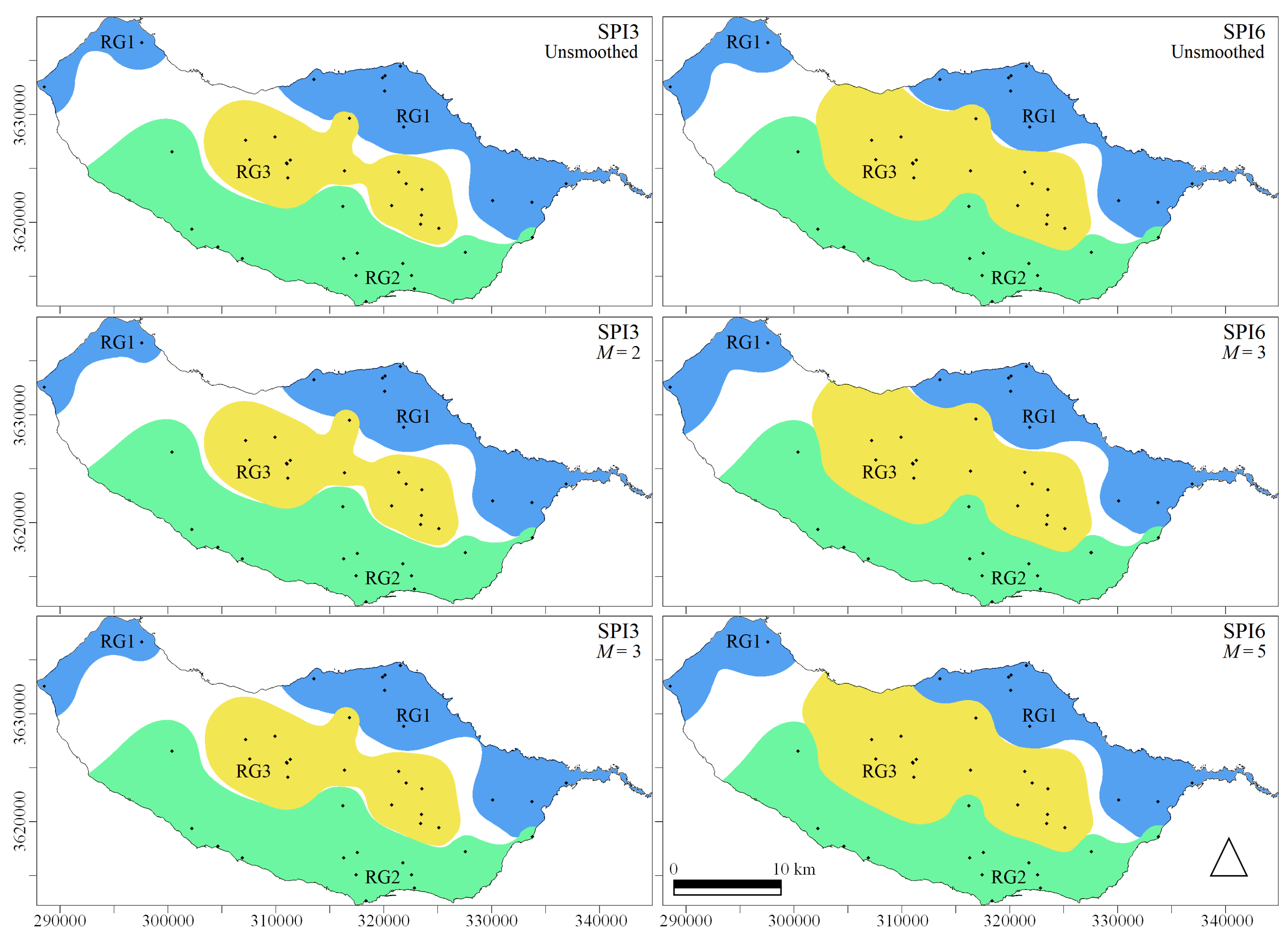
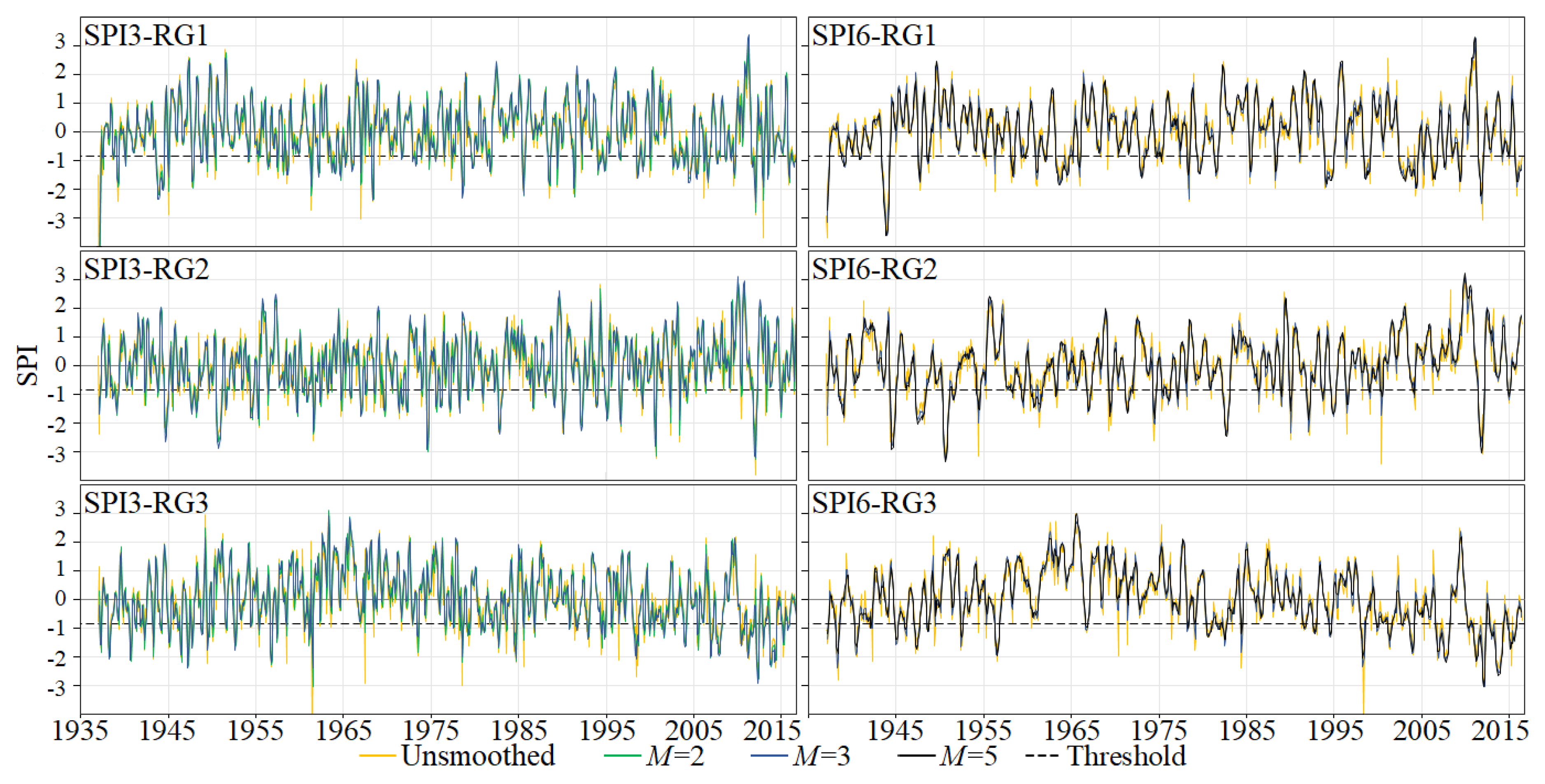
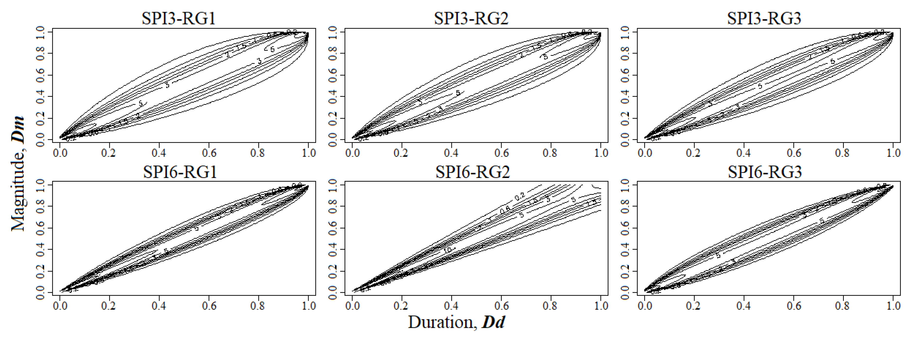
This work presents a systematic analysis of the effect of the moving average filter on drought assessment based on the SPI series (SPI3 and SPI6) from 1936 to 2016, and of the jointly modeling of drought characteristics with bivariate copulas for Madeira. The factor loadings from the factor analysis applied to unsmoothed and smoothed SPI series identified three distinct regions with different temporal patterns of the droughts: northern slope (RG1), southern slope (RG2) and central region (RG3). RG1 denotes exceptional droughts both in earlier years and at present, RG2 suffered the worst droughts in the past, while RG3 has featured more exceptional drought events from 2000 onwards. Special attention was given to this last region due to its relevance for the island’s water security, as main region for the recharge of the groundwater reservoirs.
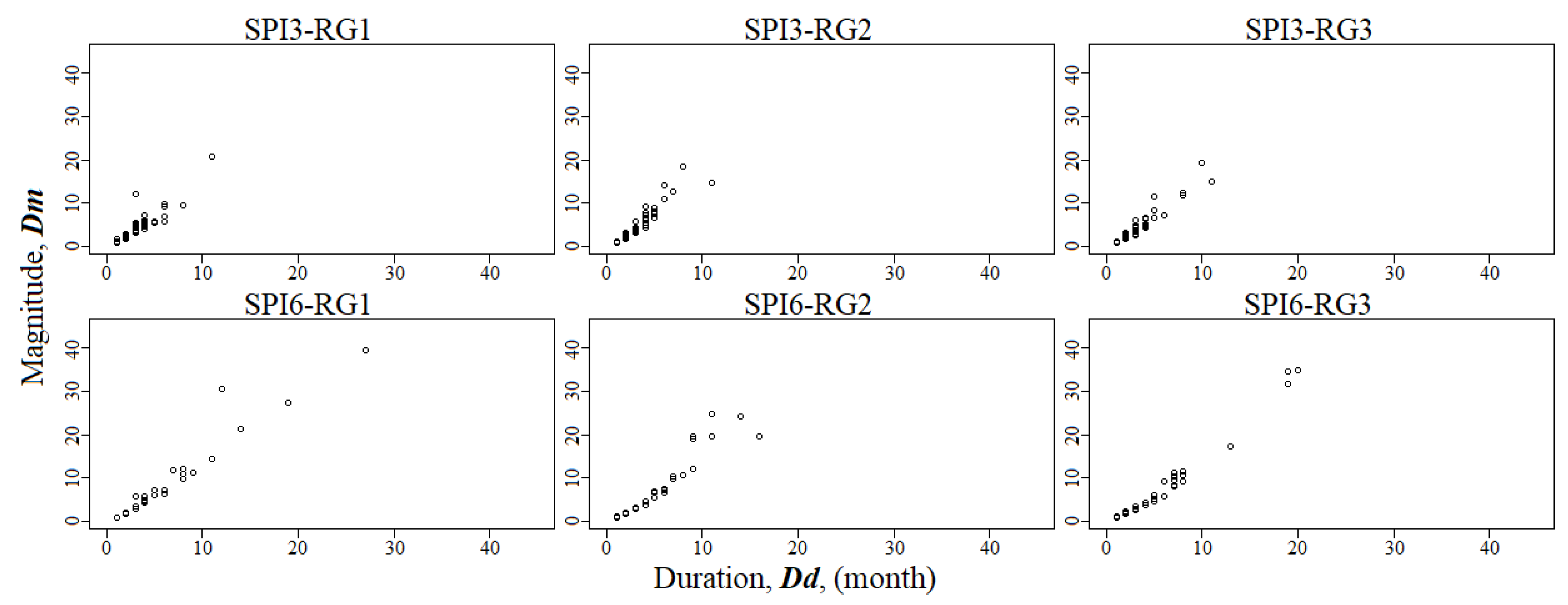
Planning and management of water resources systems under drought conditions often require the estimation of return periods of the exceptional drought events [59,85]. However, droughts are defined by multiple characteristics, some of them, presumably highly correlated. Based on the regionalized SPI series, two drought characteristics, namely drought duration ( D d ) and magnitude ( D m ) were analyzed and bivariate copulas were implemented to construct their joint distributions aiming at estimating return periods. The drought maximum intensity ( D m i , Figure 1) was not considered to avoid possible redundant information, since it is already part of the D m data, and also due to its poorly correlation with D d as stated by Sharma [91], Dracup et al. [92] and Chen et al. [87].
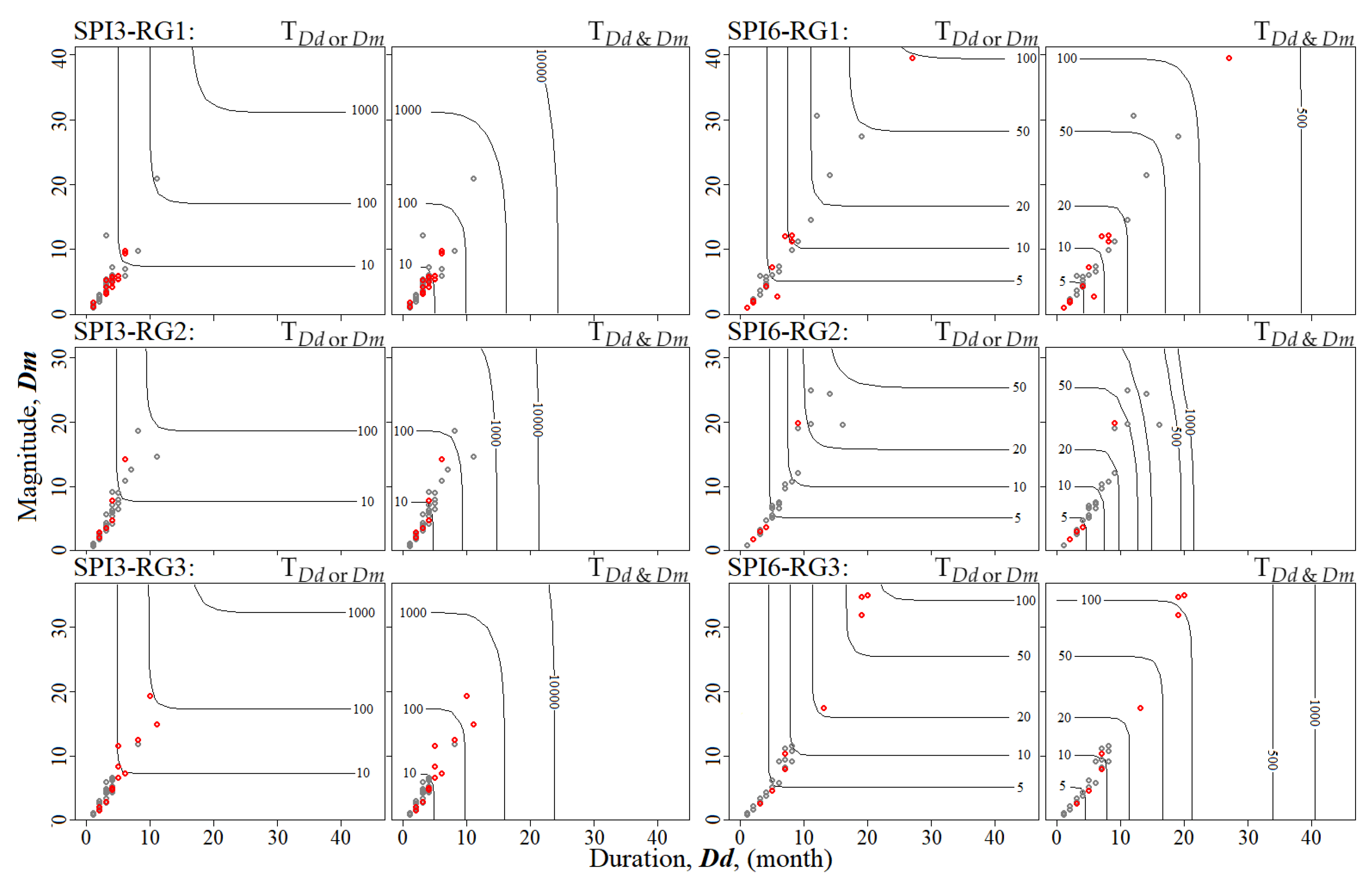
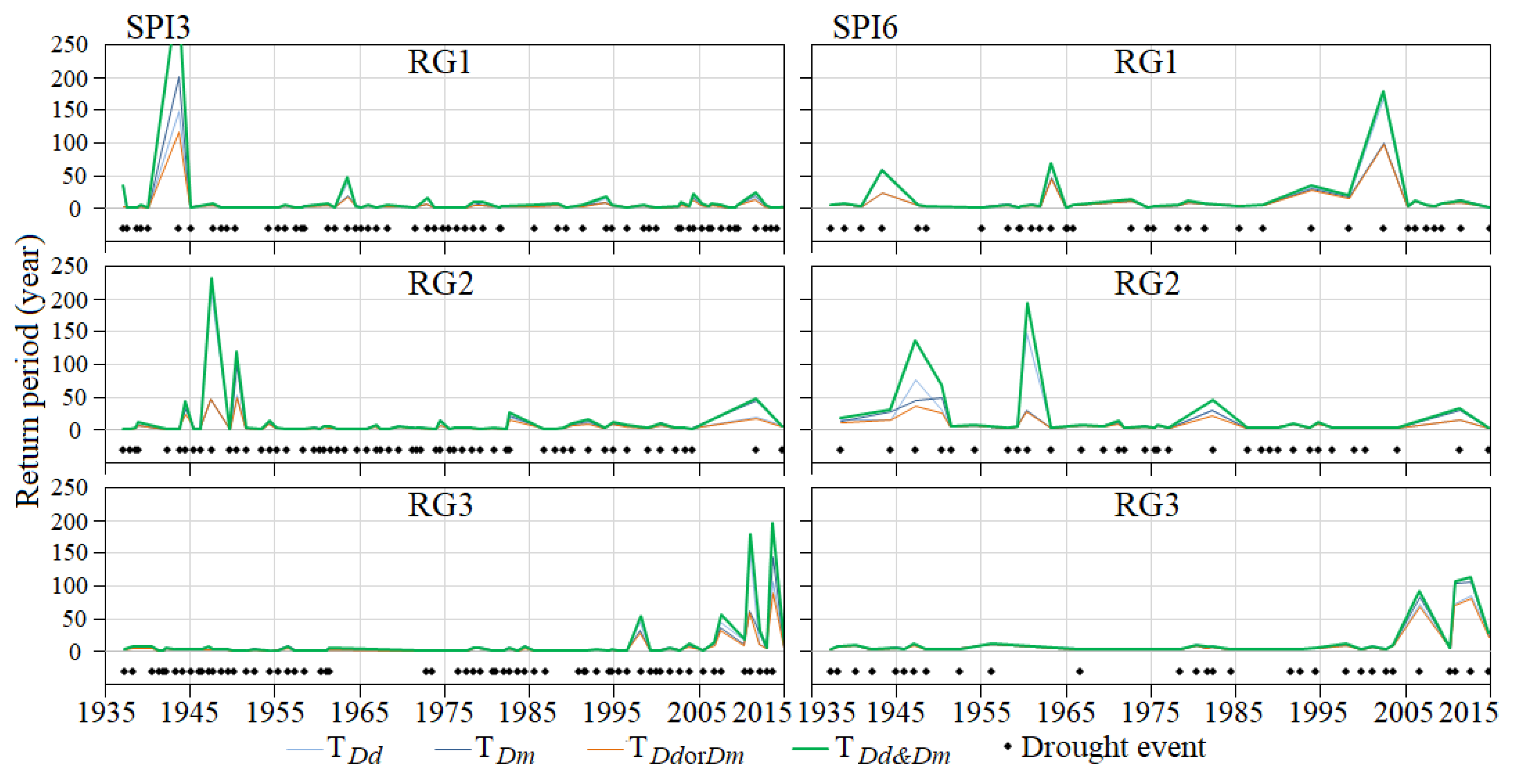
The bivariate approach enabled the generation of the joint return periods return periods between D d and D m of Figure 10. The figure shows that the events that took place more recently, namely after January 2000 (red circles), present higher or even the highest return periods, meaning that the drought events they represent were more exceptional. This is particularly evident in RG3, regardless the SPI timescale, but also in RG1, in this case only for SPI6. 
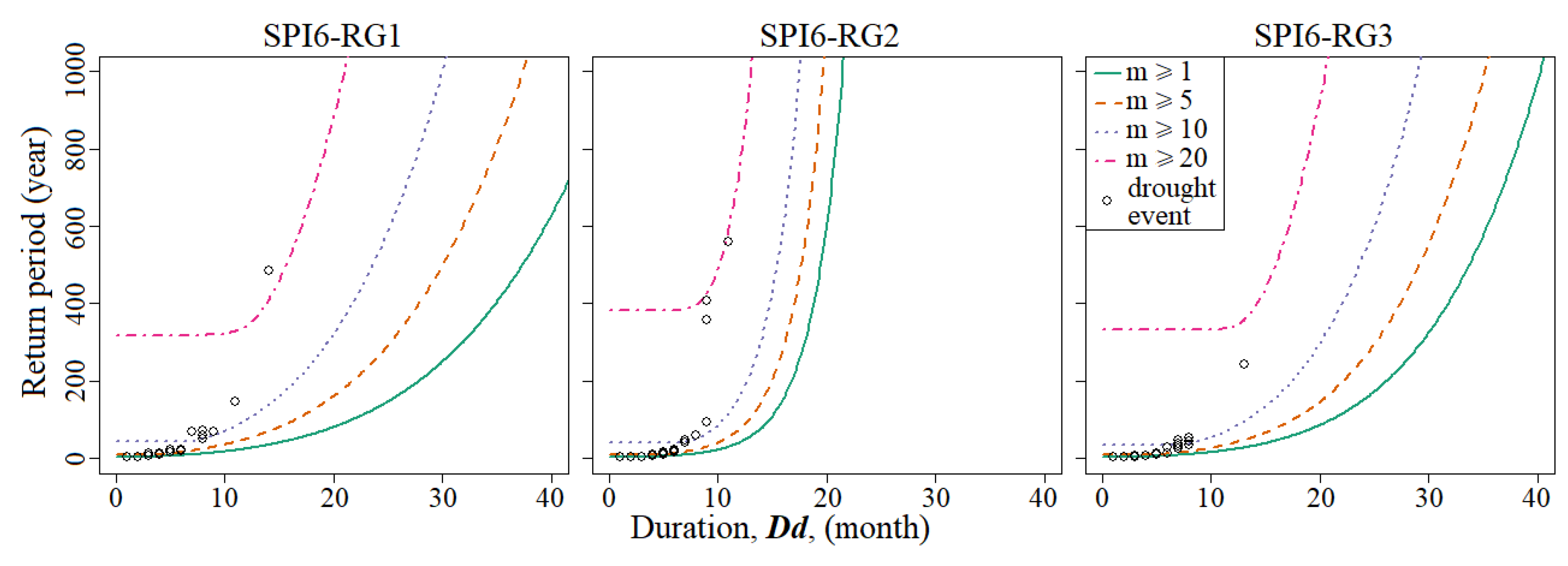
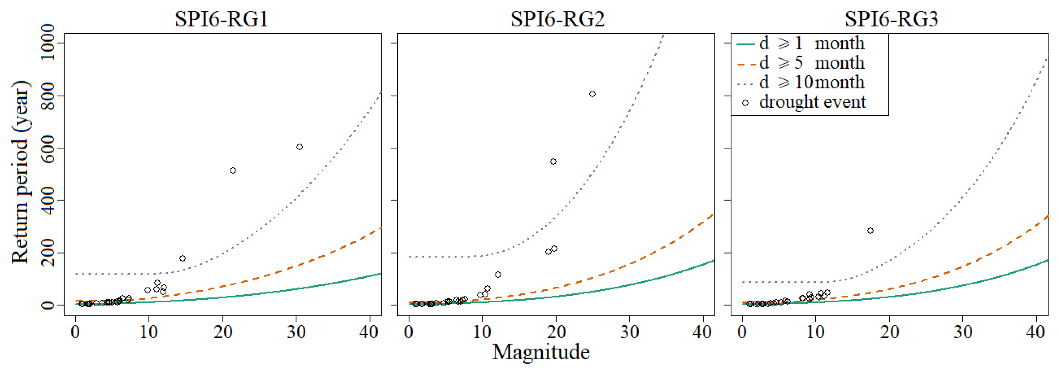
Table 8 also stresses the critical situation of RG3. In fact, from the five more exceptional drought events, regardless the SPI timescale, four took place after 2000 (more specifically after 2006). The table also shows the poorer performance of the univariate approach: in fact, for a same region and SPI timescales, all the droughts with the same duration would have the same return period, regardless the drought magnitude, and vice versa.
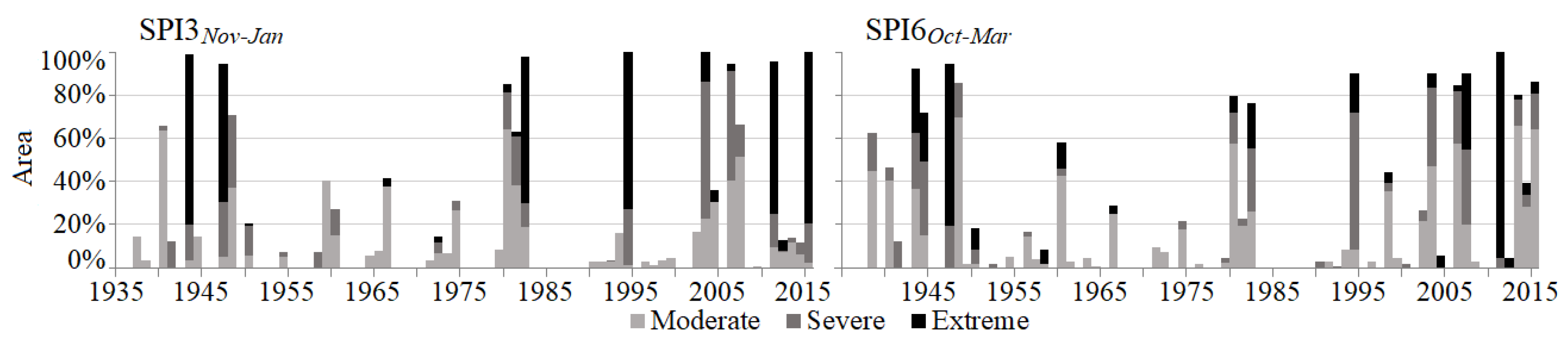
Aiming at discussing the information gained with the application of factor analysis and copulas, the results presented in Figure 13 will be compared to those from a drought characterization considering the 41 original SPI series. For that purpose, for the entire island and for each of the homogeneous regions, the yearly areas affected by moderate, severe and extreme drought were computed, based on the non-regionalized and unsmoothed SPI for wettest months of the rainy season and for the entire season itself, SPI3 N o v J a n and SPI6 O c t M a r , respectively, as shown in Figure 14 and Figure 15. The Thiessen polygon method [93] was applied to assign an areal influence (ATP from Table 1) to each rain gauge. The area attributed in each year to a specified drought category was given by the cumulative areas of the rain gauges with values of SPI within the limits of that category (
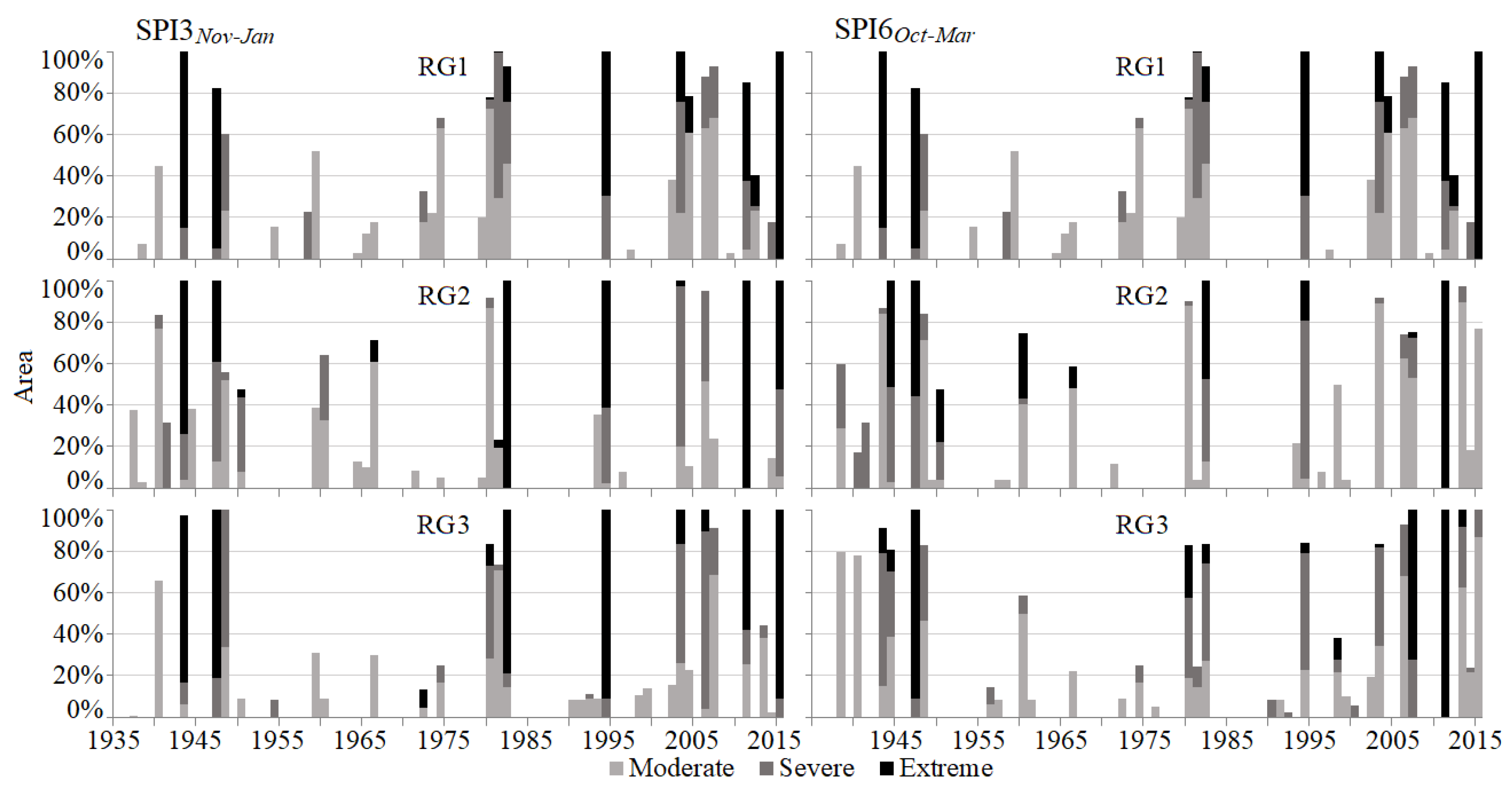
Table 2). The total areas thus achieved for each year were made dimensionless by division by the Madeira area or by the area assigned to each region, in this last case, computed based on the rain gauges located in the region.
Figure 14 and Figure 15 show that generally, the island and each of its three regions have been similarly affected in terms of percentage of the area under drought conditions. Most of the same driest spells occurred in the three regions—such as exceptionally extreme droughts of 1947, 1995, and 2011 [11]—but sometimes with different distribution of the areas assigned to the three drought categories. Figure 15 suggests that the distribution of the years with moderate, severe and extreme droughts is similar among regions for SPI3 N o v J a n . However, in the case of SPI6 O c t M a r , regardless the affected area, for RG1 and RG3 the concentration of years with severe and extreme droughts is higher in recent years (2000–2016), whereas RG2 exhibits an opposite behavior, i.e., a higher concentration of years with severe and extreme events in the past. Even though Figure 15 refers to annual series and Figure 13 to continuous series there is a certain similarity between sub-periods with more severe and extreme droughts and with the highest return periods, denoting coherence among different characterizations.
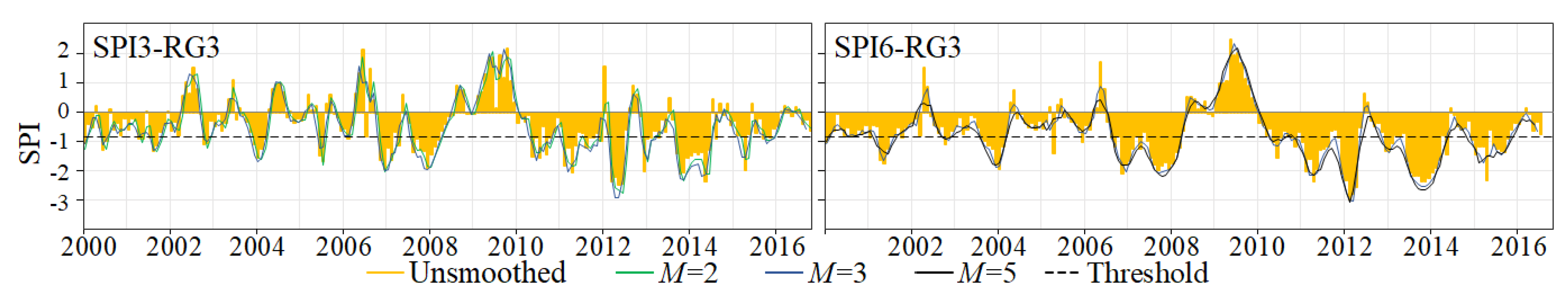
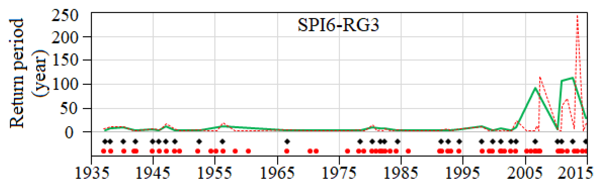
Finally, the same copula approach was applied to the regionalized unsmoothed SPI. The results for T D d & D m based on SPI6-RG3 are presented in Figure 16 which also includes the ones from the smoothed series with a running length of M = 5 . The figure confirms that smoothing the SPI series prior to factor analysis allows the elimination of the spurious drought events and/or their clustering, thus improving the visibility of the more exceptional droughts, as it happened in November 2010 and October 2012. It should be stressed that the return periods that result from the unsmoothed SPI series may be much higher than those from the smoothed series due to the higher temporal variability of the unsmoothed SPI series. The less steep response of the smoothed series compared to the one from the unsmoothed series may be because the MA filter has a good performance in the time domain (as mentioned in Section 3.2), but has a poor performance in the frequency domain [33]. Since in the present study, the response that describes how the information in the time domain (the SPI series) is being modified by the system is the important parameter and the frequency response is of little concern, this makes the MA filter applicable. In other fields of hydrology, such as in flood frequency analysis Halbert et al. [94], Archer et al. [95], the response in the frequency domain is all important, while the one in the time domain does not matter. Consequently, a frequency-domain filter may be more appropriate, e.g., the Fourier transforms [96]. Therefore, the selection of a digital filter should consider the features of the studied phenomenon.
Advances were made in the study of drought analysis based on regionalized smoothed series including on the criteria to selected the running length, M, and on the consequences of different M values. The copula approach showed that the drought events may have completely different return periods, depending on how the relationship between D d and D m is accounted for. In any case, the univariate approach only provides part of the information, often underestimating the exceptionality of the events. The use of bivariate approaches, namely based on copulas, can easily overcome such constraint.

Author Contributions

Conceptualization, L.A.E. and M.M.P.; Data curation, L.A.E.; Formal analysis, L.A.E. and J.D.P.F.; Investigation, L.A.E.; Methodology, L.A.E. and J.D.P.F.; Supervision, M.M.P. and R.R.; Visualization, L.A.E. and J.D.P.F.; Writing—original draft, L.A.E.; Writing—review & editing, M.M.P., J.D.P.F., T.M.S., T.M.d.C.S. and J.F.S.

Funding

This research received no external funding.

Acknowledgments

The work of the first author is funded by The Portuguese Foundation for Science and Technology (FCT), grant No. PD/BD/128509/2017. For the fourth author it was supported by grant from the Coordenação de Aperfeiçoamento de Pessoal de Nível Superior, Brasil (CAPES). Finance Code 001.

Conflicts of Interest

The authors declare no conflict of interest.

References

  1. Tallaksen, L.M.; Van Lanen, H. Hydrological Drought: Processes and Estimation Methods for Streamflow and Groundwater; Elsevier: Amsterdam, The Netherlands, 2004; Volume 48. [Google Scholar]
  2. Herrera, D.A.; Ault, T.R.; Fasullo, J.T.; Coats, S.J.; Carrillo, C.M.; Cook, B.I.; Williams, A.P. Exacerbation of the 2013–2016 Pan-Caribbean Drought by Anthropogenic Warming. Geophys. Res. Lett. 2018, 45, 10,619–10,626. [Google Scholar] [CrossRef]
  3. Barnett, J.; Waters, E. Rethinking the vulnerability of small island states: Climate change and development in the Pacific Islands. In The Palgrave Handbook of International Development; Springer: Berlin, Germany, 2016; pp. 731–748. [Google Scholar]
  4. Sadoff, C.W.; Borgomeo, E.; De Waal, D. Turbulent Waters: Pursuing Water Security in Fragile Contexts; World Bank: Washington, DC, USA, 2017. [Google Scholar]
  5. McCarthy, J.J.; Canziani, O.F.; Leary, N.A.; Dokken, D.J.; White, K.S. Climate change 2001: Impacts, Adaptation, and Vulnerability: Contribution of Working Group II to the Third Assessment Report of the Intergovernmental Panel on Climate Change; Cambridge University Press: Cambridge, UK, 2001; Volume 2. [Google Scholar]
  6. Parry, M.; Parry, M.L.; Canziani, O.; Palutikof, J.; Van der Linden, P.; Hanson, C. Climate Change 2007-Impacts, Adaptation and Vulnerability: Working Group II Contribution to the Fourth Assessment Report of the the Intergovernmental Panel on Climate Change; Cambridge University Press: Cambridge, UK, 2007; Volume 4. [Google Scholar]
  7. Barros, V.; Field, C.; Dokke, D.; Mastrandrea, M.; Mach, K.; Bilir, T.E.; Chatterjee, M.; Ebi, K.; Estrada, Y.; Genova, R.; et al. Climate Change 2014: Impacts, Adaptation, and Vulnerability-Part B: Regional Aspects-Contribution of Working Group II to the Fifth Assessment Report of the Intergovernmental Panel on Climate Change; Cambridge University Press: Cambridge, UK, 2014. [Google Scholar]
  8. Falkland, A.; Custodio, E. Hydrology and Water Resources of Small Islands: A Practical Guide; Number 49 in Studies and Reports in Hydrology; UNESCO: Paris, France, 1991. [Google Scholar]
  9. Nurse, L.A.; Sem, G.; Hay, J.E.; Suarez, A.G.; Wong, P.P.; Briguglio, L.; Ragoonaden, S. Small island states. Clim. Chang. 2001, 843–875. Available online: https://pdfs.semanticscholar.org/1cca/75e53f7931510a4cbdb2b8582a4e3c8e8348.pdf (accessed on 21 June 2019).
  10. Masson-Delmotte, V. Global Warming of 1.5 OC: An IPCC Special Report on the Impacts of Global Warming of 1.5C Above Pre-Industrial Levels and Related Global Greenhouse Gas Emission Pathways, in the Context of Strengthening the Global Response to the Threat of Climate Change, Sustainable Development, and Efforts to Eradicate Poverty; World Meteorological Organization: Geneva, Switzerland, 2018. [Google Scholar]
  11. Liberato, M.; Ramos, A.; Gouveia, C.; Sousa, P.; Russo, A.; Trigo, R.; Santo, F. Exceptionally extreme drought in Madeira Archipelago in 2012: Vegetation impacts and driving conditions. Agric. For. Meteorol. 2017, 232, 195–209. [Google Scholar] [CrossRef]
  12. Santos, F.; Valente, M.; Miranda, P.; Aguiar, A.; Azevedo, E.; Tomé, A.; Coelho, F. Climate change scenarios in the Azores and Madeira islands. World Resour. Rev. 2004, 16, 473–491. [Google Scholar]
  13. Tallaksen, L.M.; Hisdal, H.; Van Lanen, H.A. Space–time modelling of catchment scale drought characteristics. J. Hydrol. 2009, 375, 363–372. [Google Scholar] [CrossRef]
  14. Lloyd-Hughes, B.; Saunders, M. A drought climatology for Europe. Int. J. Climatol. 2002, 22, 1571–1592. [Google Scholar] [CrossRef]
  15. Wang, W.; Ertsen, M.W.; Svoboda, M.D.; Hafeez, M. Propagation of drought: From meteorological drought to agricultural and hydrological drought. Adv. Meteorol. 2016, 2016. [Google Scholar] [CrossRef]
  16. Van Loon, A.; Van Lanen, H.; Tallaksen, L.; Hanel, M.; Fendekova, M.; Machlica, A.; Sapriza, G.; Koutroulis, A.; Huijgevoort, M.; Jódar, J.; et al. Propagation of Drought through the Hydrological Cycle; The WATCH Project: Oxfordshire, UK, 2011. [Google Scholar]
  17. Tallaksen, L.M. Streamflow drought frequency analysis. In Drought and Drought Mitigation in Europe; Springer: Berlin, Germany, 2000; pp. 103–117. [Google Scholar]
  18. Palmer, W.C. Meteorological Drought; Research Paper No. 45; US Department of Commerce Weather Bureau: Washington, DC, USA, 1965; p. 59.
  19. Heim, R.R., Jr. A review of twentieth-century drought indices used in the United States. Bull. Am. Meteorol. Soc. 2002, 83, 1149–1165. [Google Scholar] [CrossRef]
  20. Vicente-Serrano, S.M.; Beguería, S.; López-Moreno, J.I. A multiscalar drought index sensitive to global warming: The standardized precipitation evapotranspiration index. J. Clim. 2010, 23, 1696–1718. [Google Scholar] [CrossRef]
  21. Beguería, S.; Vicente-Serrano, S.M.; Reig, F.; Latorre, B. Standardized precipitation evapotranspiration index (SPEI) revisited: parameter fitting, evapotranspiration models, tools, datasets and drought monitoring. Int. J. Climatol. 2014, 34, 3001–3023. [Google Scholar] [CrossRef]
  22. McKee, T.B.; Doesken, N.J.; Kleist, J. The relationship of drought frequency and duration to time scales. In Proceedings of the 8th Conference on Applied Climatology, Anaheim, CA, USA, 17–22 January 1993; American Meteorological Society: Boston, MA, USA, 1993; Volume 17, pp. 179–183. [Google Scholar]
  23. Demuth, S.; Stahl, K. Assessment of the Regional. Impact of Droughts in Europe (ARIDE)-Final Report; University of Freiburg/Institute of Hydrology: Freiburg im Breisgau, Germany, 2001. [Google Scholar]
  24. Vicente-Serrano, S. El Niño and La Niña influence on droughts at different timescales in the Iberian Peninsula. Water Resour. Res. 2005, 41. [Google Scholar] [CrossRef]
  25. Vicente-Serrano, S. Differences in spatial patterns of drought on different time scales: an analysis of the Iberian Peninsula. Water Resour. Manag. 2006, 20, 37–60. [Google Scholar] [CrossRef]
  26. Santos, J.; Pulido-Calvo, I.; Portela, M. Spatial and temporal variability of droughts in Portugal. Water Resour. Res. 2010, 46. [Google Scholar] [CrossRef]
  27. Svoboda, M.; Hayes, M.; Wood, D. Standardized Precipitation Index User Guide; World Meteorological Organization: Geneva, Switzerland, 2012. [Google Scholar]
  28. Yevjevich, V.M. Objective Approach to Definitions and Investigations of Continental Hydrologic Droughts, An; Hydrology Papers No. 23; Colorado State University: Fort Collins, CO, USA, 1967. [Google Scholar]
  29. Santos, J.; Portela, M.; Pulido-Calvo, I. Regional frequency analysis of droughts in Portugal. Water Resour. Manag. 2011, 25, 3537. [Google Scholar] [CrossRef]
  30. López-Moreno, J.I.; Vicente-Serrano, S.M.; Beguería, S.; García-Ruiz, J.M.; Portela, M.M.; Almeida, A. Dam effects on droughts magnitude and duration in a transboundary basin: The Lower River Tagus, Spain and Portugal. Water Resour. Res. 2009, 45. [Google Scholar] [CrossRef]
  31. Fleig, A.K.; Tallaksen, L.M.; Hisdal, H.; Demuth, S. A global evaluation of streamflow drought characteristics. Hydrol. Earth Syst. Sci. Discuss. 2006, 10, 535–552. [Google Scholar] [CrossRef]
  32. De Michele, C.; Salvadori, G.; Vezzoli, R.; Pecora, S. Multivariate assessment of droughts: Frequency analysis and dynamic return period. Water Resour. Res. 2013, 49, 6985–6994. [Google Scholar] [CrossRef]
  33. Smith, S.W. The Scientist and Engineer’s Guide to Digital Signal Processing; California Technical Publishing: Poway, CA, USA, 1997. [Google Scholar]
  34. Baeriswyl, P.A.; Rebetez, M. Regionalization of precipitation in Switzerland by means of principal component analysis. Theor. Appl. Climatol. 1997, 58, 31–41. [Google Scholar] [CrossRef]
  35. White, D.; Richman, M.; Yarnal, B. Climate regionalization and rotation of principal components. Int. J. Climatol. 1991, 11, 1–25. [Google Scholar] [CrossRef]
  36. Briggs, R.; Lemin, J. Delineation of climatic regions in Maine. Can. J. For. Res. 1992, 22, 801–811. [Google Scholar] [CrossRef]
  37. Corte-Real, J.; Qian, B.; Xu, H. Regional climate change in Portugal: Precipitation variability associated with large-scale atmospheric circulation. Int. J. Climatol. 1998, 18, 619–635. [Google Scholar] [CrossRef]
  38. Unal, Y.; Kindap, T.; Karaca, M. Redefining the climate zones of Turkey using cluster analysis. Int. J. Climatol. 2003, 23, 1045–1055. [Google Scholar] [CrossRef]
  39. Vicente-Serrano, S. Las sequías climáticas en el valle medio del Ebro: Factores atmosféricos, evolución temporal y variabilidad espacial; Consejo de Protección de la Naturaleza de Aragón: 2005. Zaragoza, Spain, 2005. [Google Scholar]
  40. Raziei, T.; Martins, D.; Bordi, I.; Santos, J.; Portela, M.M.; Pereira, L.; Sutera, A. SPI Modes of Drought Spatial and Temporal Variability in Portugal: Comparing Observations, PT02 and GPCC Gridded Datasets. Water Resour. Manag. 2015, 29, 487–504. [Google Scholar] [CrossRef]
  41. Chebana, F.; Ouarda, T.B. Multivariate quantiles in hydrological frequency analysis. Environmetrics 2011, 22, 63–78. [Google Scholar] [CrossRef]
  42. Shiau, J.T. Fitting drought duration and severity with two-dimensional copulas. Water Resour. Manag. 2006, 20, 795–815. [Google Scholar] [CrossRef]
  43. Chazarra, A.; Mestre, A.; Pires, V.; Cunha, S.; Silva, A.; Marques, J.; Carvalho, F.; Mendes, M.; Neto, J.; Mendes, L.; et al. Climate Atlas of the Achipelagos of the Canary Islands, Madeira and the Azores: Air Temperature and Precipitation (1971–2000); Production Department of the State Meteorological Agency of Spain: Madrid, Spain, 2011; pp. 15–62. [Google Scholar]
  44. Fragoso, M.; Trigo, R.; Pinto, J.; Lopes, S.; Lopes, A.; Ulbrich, S.; Magro, C. The 20 February 2010 Madeira flash-floods: Synoptic analysis and extreme rainfall assessment. Nat. Hazards Earth Syst. Sci. 2012, 12, 715–730. [Google Scholar] [CrossRef]
  45. Prada, S.N.; Da Silva, M.O.; Cruz, J.V. Groundwater behaviour in Madeira, volcanic island (Portugal). Hydrogeol. J. 2005, 13, 800–812. [Google Scholar] [CrossRef]
  46. Duarte, R. Prospecção e captação de águas subterrâneas em terrenos vulcânicos, arquipélago da Madeira. 4º Congresso da Água-A Água como Recurso Estruturante do Desenvolvimento” Coimbra 1998. Available online: http://www.aprh.pt/congressoagua98/Index.htm (accessed on 25 June 2019).
  47. Espinosa, L.A.; Portela, M.M.; Rodrigues, R. Spatio-temporal variability of droughts over past 80 years in Madeira Island. J. Hydrol. Reg. Stud. 2019, 25, 100623. [Google Scholar] [CrossRef]
  48. Van-Buuren, S.; Groothuis-Oudshoorn, K. mice: Multivariate imputation by chained equations in R. J. Stat. Softw. 2010, 1–68. [Google Scholar] [CrossRef]
  49. Edwards, D.C.; McKee, T. Characteristics of 20th Century Drought in the United States at Multiple Time Scales; Dept. of Atmospheric Science, Colorado State University: Fort Collins, CO, USA, 1997; Volume 2. [Google Scholar]
  50. Hayes, M.J.; Svoboda, M.D.; Wiihite, D.A.; Vanyarkho, O.V. Monitoring the 1996 drought using the standardized precipitation index. Bull. Am. Meteorol. Soc. 1999, 80, 429–438. [Google Scholar] [CrossRef]
  51. Agnew, C. Using the SPI to identify drought. Drought Netw. News 2000, 12. Available online: https://digitalcommons.unl.edu/cgi/viewcontent.cgi?article=1000&context=droughtnetnews (accessed on 21 June 2019).
  52. Tallaksen, L.M.; Madsen, H.; Clausen, B. On the definition and modelling of streamflow drought duration and deficit volume. Hydrol. Sci. J. 1997, 42, 15–33. [Google Scholar] [CrossRef]
  53. Zelenhasić, E.; Salvai, A. A method of streamflow drought analysis. Water Resour. Res. 1987, 23, 156–168. [Google Scholar] [CrossRef]
  54. Byzedi, M.; Saghafian, B. Analysis of hydrological drought based on daily flow series. Proc. World Acad. Sci. Eng. Technol 2010, 70, 249–252. [Google Scholar]
  55. Li, S.; Xiong, L.; Dong, L.; Zhang, J. Effects of the Three Gorges Reservoir on the hydrological droughts at the downstream Yichang station during 2003–2011. Hydrol. Process. 2013, 27, 3981–3993. [Google Scholar] [CrossRef]
  56. Shin, J.Y.; Chen, S.; Lee, J.H.; Kim, T.W. Investigation of drought propagation in South Korea using drought index and conditional probability. Terr. Atmos. Ocean. Sci. 2018, 29. [Google Scholar] [CrossRef] [Green Version]
  57. Golestan, S.; Ramezani, M.; Guerrero, J.M.; Freijedo, F.D.; Monfared, M. Moving average filter based phase-locked loops: Performance analysis and design guidelines. IEEE Trans. Power Electron. 2013, 29, 2750–2763. [Google Scholar] [CrossRef] [Green Version]
  58. Hair, J.; Black, W.; Babin, B.; Anderson, R.; Tatham, R. Multivariate Data Analysis; Prentice Hall: Upper Saddle River, NJ, USA, 1998; Volume 5, pp. 207–219. [Google Scholar]
  59. Bonaccorso, B.; Bordi, I.; Cancelliere, A.; Rossi, G.; Sutera, A. Spatial variability of drought: An analysis of the SPI in Sicily. Water Resour. Manag. 2003, 17, 273–296. [Google Scholar] [CrossRef]
  60. Raziei, T.; Saghafian, B.; Paulo, A.A.; Pereira, L.S.; Bordi, I. Spatial patterns and temporal variability of drought in western Iran. Water Resour. Manag. 2009, 23, 439. [Google Scholar] [CrossRef]
  61. Deng, X.; Tian, X. Entropy principal component analysis and its application to nonlinear chemical process fault diagnosis. Asia-Pac. J. Chem. Eng. 2014, 9, 696–706. [Google Scholar] [CrossRef]
  62. Shannon, C.E. A mathematical theory of communication. Bell Syst. Tech. J. 1948, 27, 379–423. [Google Scholar] [CrossRef] [Green Version]
  63. Kaiser, H.F. The application of electronic computers to factor analysis. Educ. Psychol. Meas. 1960, 20, 141–151. [Google Scholar] [CrossRef]
  64. Abdi, H. Factor rotations in factor analyses. Encyclopedia for Research Methods for the Social Sciences; Sage: Thousand Oaks, CA, USA, 2003; pp. 792–795. [Google Scholar]
  65. Rencher, A.C. Methods of Multivariate Analysis, 2nd ed.; John Wiley & Sons: Hoboken, NJ, USA, 2002; Volume 492, pp. 380–404. [Google Scholar]
  66. Grice, J.W. Computing and evaluating factor scores. Psychol. Methods 2001, 6, 430. [Google Scholar] [CrossRef] [PubMed]
  67. Ayantobo, O.O.; Li, Y.; Song, S. Multivariate drought frequency analysis using four-variate symmetric and asymmetric Archimedean copula functions. Water Resour. Manag. 2018, 33, 103–127. [Google Scholar] [CrossRef] [Green Version]
  68. Montaseri, M.; Amirataee, B.; Rezaie, H. New approach in bivariate drought duration and severity analysis. J. Hydrol. 2018, 559, 166–181. [Google Scholar] [CrossRef]
  69. Zhang, L.; Singh, V.P. Bivariate rainfall frequency distributions using Archimedean copulas. J. Hydrol. 2007, 332, 93–109. [Google Scholar] [CrossRef]
  70. Goel, N.; Seth, S.; Chandra, S. Multivariate modeling of flood flows. J. Hydraul. Eng. 1998, 124, 146–155. [Google Scholar] [CrossRef]
  71. Shiau, J.T. Return period of bivariate distributed extreme hydrological events. Stoch. Environ. Res. Risk Assess. 2003, 17, 42–57. [Google Scholar] [CrossRef]
  72. Bacchi, B.; Becciu, G.; Kottegoda, N.T. Bivariate exponential model applied to intensities and durations of extreme rainfall. J. Hydrol. 1994, 155, 225–236. [Google Scholar] [CrossRef]
  73. Salas, J.D.; Fu, C.; Cancelliere, A.; Dustin, D.; Bode, D.; Pineda, A.; Vincent, E. Characterizing the severity and risk of drought in the Poudre River, Colorado. J. Water Resour. Plan. Manag. 2005, 131, 383–393. [Google Scholar] [CrossRef]
  74. González, J.; Valdés, J.B. Bivariate drought recurrence analysis using tree ring reconstructions. J. Hydrol. Eng. 2003, 8, 247–258. [Google Scholar] [CrossRef]
  75. Kao, S.C.; Govindaraju, R.S. A copula-based joint deficit index for droughts. J. Hydrol. 2010, 380, 121–134. [Google Scholar] [CrossRef]
  76. Xu, K.; Yang, D.; Xu, X.; Lei, H. Copula based drought frequency analysis considering the spatio-temporal variability in Southwest China. J. Hydrol. 2015, 527, 630–640. [Google Scholar] [CrossRef]
  77. Chang, J.; Li, Y.; Wang, Y.; Yuan, M. Copula-based drought risk assessment combined with an integrated index in the Wei River Basin, China. J. Hydrol. 2016, 540, 824–834. [Google Scholar] [CrossRef]
  78. Fan, L.; Wang, H.; Liu, Z.; Li, N. Quantifying the relationship between drought and water scarcity using Copulas: Case study of Beijing–Tianjin–Hebei metropolitan areas in China. Water 2018, 10, 1622. [Google Scholar] [CrossRef] [Green Version]
  79. Pontes Filho, J.D.; Portela, M.M.; Marinho de Carvalho Studart, T.; Souza Filho, F.d.A. A Continuous Drought Probability Monitoring System, CDPMS, Based on Copulas. Water 2019, 11, 1925. [Google Scholar] [CrossRef] [Green Version]
  80. Sharifi, E.; Saghafian, B.; Steinacker, R. Copula-based stochastic uncertainty analysis of satellite precipitation products. J. Hydrol. 2019, 570, 739–754. [Google Scholar] [CrossRef]
  81. Sklar, M. Fonctions de repartition an dimensions et leurs marges. Publ. Inst. Statist. Univ. Paris 1959, 8, 229–231. [Google Scholar]
  82. Nelsen, R.B. An Introduction to Copulas; Springer Science & Business Media: Berlin, Germany, 2007. [Google Scholar]
  83. Joe, H. Multivariate Models and Multivariate Dependence Concepts; CRC Press: Boca Raton, FL, USA, 1997. [Google Scholar]
  84. Brechmann, E.; Schepsmeier, U. Cdvine: Modeling dependence with c-and d-vine copulas in r. J. Stat. Softw. 2013, 52, 1–27. [Google Scholar] [CrossRef] [Green Version]
  85. Shiau, J.T.; Shen, H.W. Recurrence analysis of hydrologic droughts of differing severity. J. Water Resour. Plan. Manag. 2001, 127, 30–40. [Google Scholar] [CrossRef]
  86. Kwon, H.H.; Lall, U. A copula-based nonstationary frequency analysis for the 2012–2015 drought in California. Water Resour. Res. 2016, 52, 5662–5675. [Google Scholar] [CrossRef] [Green Version]
  87. Chen, L.; Singh, V.P.; Guo, S.; Mishra, A.K.; Guo, J. Drought analysis using copulas. J. Hydrol. Eng. 2012, 18, 797–808. [Google Scholar] [CrossRef]
  88. Tosunoglu, F.; Can, I. Application of copulas for regional bivariate frequency analysis of meteorological droughts in Turkey. Nat. Hazards 2016, 82, 1457–1477. [Google Scholar] [CrossRef]
  89. Burrough, P.; McDonnell, R. Spatial Information Systems and Geostatistics. In Principle of Geographic Information Systems; Oxford University Press: Oxford, UK, 1998; Volume 333. [Google Scholar]
  90. Venter, G. Tails of Copulas. Proc. Casualty Actuar. Soc. 2002, 89. Available online: https://www.casact.org/library/studynotes/Venter_Tails_of_Copulas.pdf (accessed on 20 August 2019).
  91. Sharma, T. A drought frequency formula. Hydrol. Sci. J. 1997, 42, 803–814. [Google Scholar] [CrossRef]
  92. Dracup, J.A.; Lee, K.S.; Paulson, E.G., Jr. On the definition of droughts. Water Resour. Res. 1980, 16, 297–302. [Google Scholar] [CrossRef]
  93. Thiessen, A.H. Precipitation averages for large areas. Mon. Weather Rev. 1911, 39, 1082–1089. [Google Scholar] [CrossRef]
  94. Halbert, K.; Nguyen, C.C.; Payrastre, O.; Gaume, E. Reducing uncertainty in flood frequency analyses: A comparison of local and regional approaches involving information on extreme historical floods. J. Hydrol. 2016, 541, 90–98. [Google Scholar] [CrossRef]
  95. Archer, D.R.; Parkin, G.; Fowler, H.J. Assessing long term flash flooding frequency using historical information. Hydrol. Res. 2016, 48, 1–16. [Google Scholar] [CrossRef] [Green Version]
  96. Bracewell, R.N.; Bracewell, R.N. The Fourier Transform and Its Applications; McGraw-Hill: New York, NY, USA, 1986; Volume 31999. [Google Scholar]
Figure 1. Run theory and definition of drought characteristics— D d , D m , D m i , L for SPI values below an adopted threshold, u. Adapted from Santos et al. [29].
Water 11 02489 g001
Figure 2. Location of the 41 rain gauges of Table 1 over the surface of the average rainfall referred to the hydrological year, HDY. Adapted from Espinosa et al. [47].
Water 11 02489 g002
Figure 3. Spatial distribution of the homogeneous regions based on the factor loadings (correlation coefficients) higher than 0.60. The regions RG1, RG2, and RG3, are related to F1, F2, and F3, respectively.
Water 11 02489 g003
Figure 4. January 1937 to December 2016. F1 (RG1-northern slope), F2 (RG2-southern slope) and F3 (RG3-central region) from the series of SPI3 (left figures with unsmoothed series and with running lengths, M, of 2 and 3) and of SPI6 (right figures with also unsmoothed series and with M of 3 and 5).
Water 11 02489 g004
Figure 5. January 2000 to December 2016. F3 (RG3-central region) from the SPI3 (left for unsmoothed series and M of 2 and 3) and the SPI6 series (right for unsmoothed series and M of 3 and 5).
Water 11 02489 g005
Figure 6. Number of months under drought conditions from January 2000 to December 2016 for the regionalized SPI3 (left figures) and SPI6 (right figures) at the central region.
Water 11 02489 g006
Figure 7. D d and D m of the drought events for the regionalized unsmoothed and smoothed series with different running lengths for SPI3 (left figures) and SPI6 (right figures) series in the central region (RG3).
Water 11 02489 g007
Figure 8. Scatter plots between D d and D m obtained from the regionalized SPI3 (with M = 3 ) and SPI6 (with M = 5 ) series, for the different regions.
Water 11 02489 g008
Figure 9. Joint cumulative distribution functions of the best-fitted copula of normalized drought duration and magnitude for each region and timescale of SPI.
Water 11 02489 g009
Figure 10. Joint return periods, T D d or D m , T D d & D m for each region and SPI timescale. The drought events that started between January 1937 and December 1999 are represented by grey circles, and those with start from January 2000 on, by red circles.
Water 11 02489 g010
Figure 11. Conditional return period T D d D m m for different drought magnitudes (denoted by m) for SPI6 in the three regions.
Water 11 02489 g011
Figure 12. Conditional return period T D m D d d for different drought duration (denoted by d) for SPI6 in the three regions.
Water 11 02489 g012
Figure 13. Univariate, and bivariate return period ( T D d , T D m , T D d or D m , T D d & D m ) for SPI3 (left figures with M = 3 ) and SPI6 (right figures with M = 5 ). The start date of each drought event is represented by the location of the black bullet.
Water 11 02489 g013
Figure 14. SPI3 N o v J a n (left figure) and SPI6 O c t M a r (right figure) series. Yearly area of Madeira affected by the different drought categories (740.63 km 2 —41 rain gauges).
Water 11 02489 g014
Figure 15. SPI3 N o v J a n (left figures) and SPI6 O c t M a r (right figures) series. For each region, yearly area affected by the different drought categories (RG1 with 232.35 km 2 —11 rain gauges, RG2 with 281.18 km 2 —14 rain gauges, and RG3 with 227.10 km 2 —16 rain gauges).
Water 11 02489 g015
Figure 16. The central region. The start of drought events and their associated bivariate return period T D d & D m for SPI6 series without smoothing (dashed line and red bullets) and with M = 5 (solid line and black bullets).
Water 11 02489 g016
Table 1. The 41 rain gauges adopted in the study. Identification (code and name), WGSM84 coordinates, elevation, average annual rainfalls from October 1937 to September 2016 (hydrological years) (HDY), areal influence (ATP) according to the Thiessen polygons method, and homogeneous regions (RG1, RG2, RG3) to which they belong. Adapted from Espinosa et al. [47].
CodeNameLat-NLon-WElev. (m.a.s.l.)HDY (mm)ATP (km 2 )Region
M01Areeiro32.7200−16.91701610.002592.2013.67RG3
M02Bica da Cana32.7562−17.05541560.002605.7022.06RG3
M03Camacha-Valparaiso32.6763−16.8421675.001406.8028.58RG2
M04Encumeada de São Vicente32.7503−17.0169900.002410.501.12RG3
M05Funchal Observatório32.6476−16.892458.00608.407.08RG2
M06Lugar de Baixo32.6790−17.083215.00597.7010.94RG2
M07Ponta Delgada32.8213−16.9920123.001070.2017.27RG1
M08Sanatório32.6687−16.9006384.00809.7011.76RG2
M09Santana32.7220−16.774280.001338.9016.47RG1
M10Canhas32.6942−17.1098400.00779.2025.20RG2
M11Caniçal32.7374−16.738715.00674.6011.35RG1
M12Caramujo32.7694−17.05851214.002653.0030.43RG3
M13Curral das Freiras32.7456−16.9599787.001754.7020.09RG3
M14Loural32.7727−17.0292368.001600.6019.38RG3
M16Montado do Pereiro32.7019−16.88391260.002080.406.54RG3
M18Ponta do Pargo32.8108−17.2589339.00817.8040.68RG1
M19Porto do Moniz32.8492−17.162864.001234.2052.22RG1
M20Queimadas32.7831−16.9022881.002207.3034.68RG1
M21Rabaçal32.7585−17.13111233.002005.3088.95RG2
M22Ribeira Brava32.6740−17.063025.00703.1024.14RG2
M23Ribeiro Frio32.7309−16.88301167.002276.1019.08RG3
M24Santo António32.6768−16.9459525.00929.8010.83RG2
M25Santo da Serra32.7260−16.8170660.001790.1036.10RG1
M26Bom Sucesso32.6620−16.8960291.00719.606.98RG2
M27Santa Catarina32.6936−16.773149.00660.307.75RG2
M28Cascalho32.8290−16.9250430.001537.801.83RG1
M29Poiso e Posto Florestal32.7130−16.88701360.002134.504.60RG3
M30Vale da Lapa32.8270−16.9280346.001882.305.32RG1
M32Lapa Branca-Curral das Freiras32.7190−16.9650610.001360.0022.46RG2
M34Serra de Água32.7420−17.0200573.001971.0024.35RG3
M35Chão dos Louros E.32.7570−17.0180895.002509.709.55RG3
M37Lombo Furão32.7490−16.9110994.002416.2013.62RG3
M43Meia Serra32.7020−16.8700115.002444.0012.48RG3
M44Covão ETA32.6750−16.9630510.00930.3022.46RG2
M45Encumeadas Casa EEM32.7540−17.02101010.002202.402.32RG3
M46Santa Quitéria ETA32.6610−16.9510320.00726.509.20RG2
M48ETA São Jorge32.8160−16.9260500.002093.7010.43RG1
M49Fajã Penedo32.7920−16.9600620.002378.8023.84RG3
M50Cabeço do Meio-Nogueira32.7357−16.8987995.002477.904.08RG3
M51Ponta de São Jorge32.8337−16.9067266.00779.306.15RG1
M53Lido-Cais do Carvão32.6366−16.936520.00340.104.99RG2
Table 2. Drought categories and associated non-exceedance probability based on SPI. Adapted from Agnew [51].
CategoryProbabilitySPI
No drought0.60 0.84 and <0.84
Moderate drought0.20< 0.84
Severe drought0.10< 1.28
Extreme drought0.05< 1.65
Table 3. Copula candidate family and mathematical formulation.
Copula FamilyMathematical Formulation
Meta-ellipticGaussian ϕ ρ ( ϕ 1 ( u 1 ) , ϕ 1 ( u 2 ) )
t-Student T ρ , v ( T v 1 ( u 1 ) , T v 1 ( u 2 ) )
Clayton ( u 1 θ + u 2 θ 1 ) 1 θ
ArchimedeanFrank θ 1 log 1 + ( e θ u 1 1 ) ( e θ u 2 1 ) ( e θ 1 )
Gumbel exp ( [ ( ln u 1 ) θ + ( ln u 2 ) θ ] 1 θ )
Table 4. Eigenvalues ( λ ) of each factor (F) from the factor analysis associated with the unrotated solution for different timescale of SPI and running length (M). %Var represents the explained variance calculated by dividing λ by the number of variables, i.e., 41.
FactorSPI3 UnsmoothedSPI3 with M = 2 SPI3 with M = 3 SPI6 UnsmoothedSPI6 with M = 3 SPI6 with M = 5
λ %Var Σ %Var λ %Var Σ %Var λ %Var Σ %Var λ %Var Σ %Var λ %Var Σ %Var λ %Var Σ %Var
131.4776.7676.7631.4876.7776.7731.2876.2976.2931.6977.3077.3031.4076.5876.5831.0075.6275.62
22.425.9182.672.415.8782.642.395.8482.132.235.4382.732.265.5182.092.305.6181.23
31.062.5985.261.072.6185.251.102.6984.821.132.7785.501.182.8984.981.243.0284.25
40.651.5986.850.681.6786.920.741.8086.620.811.9787.470.902.1987.171.002.4386.68
50.581.4288.270.591.4588.370.601.4788.090.631.5489.010.661.6188.780.721.7588.43
390.020.0585.170.020.0485.180.020.0484.760.020.0585.420.010.0284.940.010.0284.22
400.020.0585.220.020.0485.220.010.0384.800.010.0285.470.010.0284.960.010.0284.24
410.020.0485.260.010.0385.250.010.0284.820.010.0285.490.010.0184.970.000.0184.25
Table 5. Factor loadings (correlation coefficients) from the factor analysis associated with the rotated solution for different timescales of SPI and running lengths (M). Correlations equal or higher than 0.60 are marked with an asterisk (*). Smaller factor loadings were assumed to be uncorrelated with their respective F. The rain gauges are sorted in terms of the proposed regionalization.
RegionCodeSPI3 UnsmoothedSPI3 with M = 2 SPI3 with M = 3 SPI6 UnsmoothedSPI6 with M = 3 SPI6 with M = 5
F1F2F3F1F2F3F1F2F3F1F2F3F1F2F3F1F2F3
RG1M07*0.750.410.39*0.750.410.39*0.740.400.41*0.730.410.43*0.710.400.45*0.700.400.47
M09*0.880.260.22*0.880.260.22*0.880.260.23*0.870.270.24*0.870.260.25*0.870.250.27
M11*0.650.540.28*0.650.550.28*0.640.550.29*0.620.520.31*0.600.530.32*0.610.520.33
M18*0.610.450.38*0.600.440.39*0.700.420.40*0.620.340.45*0.700.300.46*0.600.270.48
M19*0.610.380.39*0.600.360.40*0.630.350.42*0.610.350.42*0.610.340.44*0.620.330.46
M20*0.760.240.39*0.750.240.40*0.740.240.41*0.720.240.40*0.710.230.41*0.690.220.42
M25*0.700.310.40*0.680.310.42*0.670.310.43*0.660.300.43*0.640.300.43*0.620.290.44
M28*0.800.280.43*0.790.280.44*0.770.280.46*0.770.300.46*0.750.300.49*0.720.300.51
M30*0.760.320.49*0.760.310.50*0.740.310.51*0.740.310.51*0.720.300.53*0.700.290.52
M48*0.830.320.33*0.820.330.34*0.810.330.34*0.800.350.33*0.790.360.33*0.780.370.33
M51*0.800.410.19*0.810.410.18*0.810.410.17*0.810.410.18*0.820.400.17*0.820.390.16
RG2M030.38*0.650.480.37*0.650.480.36*0.640.480.38*0.640.500.37*0.640.490.37*0.640.48
M050.35*0.850.270.35*0.850.280.35*0.850.290.35*0.840.330.33*0.850.330.32*0.850.33
M060.28*0.840.270.28*0.840.270.29*0.840.280.30*0.830.290.30*0.830.290.30*0.830.30
M080.36*0.770.370.37*0.770.370.36*0.760.380.36*0.760.400.35*0.760.410.34*0.760.41
M100.32*0.810.380.32*0.810.380.32*0.810.380.33*0.800.400.33*0.800.400.33*0.800.40
M210.39*0.630.550.39*0.640.560.39*0.630.560.39*0.640.520.39*0.630.520.38*0.620.52
M220.28*0.850.300.27*0.850.290.27*0.860.290.29*0.850.290.27*0.860.280.25*0.860.27
M240.27*0.790.450.27*0.790.450.26*0.790.460.29*0.780.490.27*0.770.500.25*0.770.50
M260.37*0.800.360.37*0.810.370.36*0.810.380.35*0.810.410.34*0.810.420.33*0.810.43
M270.54*0.610.360.55*0.600.360.55*0.600.360.53*0.620.400.52*0.630.400.51*0.640.40
M320.36*0.680.460.36*0.680.460.35*0.680.470.34*0.680.490.33*0.680.500.31*0.670.50
M440.31*0.820.400.31*0.820.400.31*0.820.410.32*0.810.440.31*0.810.440.31*0.810.44
M460.33*0.860.320.32*0.860.320.32*0.860.320.33*0.860.330.32*0.870.330.31*0.870.32
M530.38*0.840.270.38*0.850.270.37*0.850.270.36*0.860.280.35*0.860.280.34*0.870.28
RG3M010.420.45*0.680.410.44*0.690.390.42*0.710.390.38*0.730.370.36*0.750.340.34*0.76
M020.440.37*0.710.440.37*0.710.420.37*0.720.390.38*0.730.370.37*0.750.350.37*0.75
M040.470.50*0.620.470.50*0.630.460.50*0.640.440.51*0.650.430.51*0.670.410.50*0.69
M120.500.46*0.620.500.46*0.620.490.46*0.620.470.46*0.630.470.44*0.630.460.43*0.64
M130.300.53*0.620.300.59*0.620.290.52*0.630.330.53*0.680.330.53*0.690.320.55*0.70
M140.500.51*0.610.510.51*0.640.500.51*0.660.520.50*0.620.510.49*0.620.500.49*0.63
M160.460.50*0.640.460.50*0.640.450.50*0.650.460.50*0.660.440.49*0.670.420.49*0.68
M230.520.33*0.630.540.32*0.690.520.32*0.700.510.36*0.660.490.36*0.600.460.36*0.60
M290.480.41*0.670.470.40*0.680.450.38*0.700.450.39*0.700.420.38*0.720.400.38*0.74
M340.420.55*0.610.420.55*0.640.410.55*0.670.400.53*0.680.390.53*0.680.380.53*0.68
M350.440.47*0.710.440.47*0.710.430.46*0.710.410.46*0.730.400.45*0.740.390.45*0.75
M370.540.43*0.640.540.44*0.640.530.44*0.640.520.47*0.630.500.47*0.640.480.48*0.64
M430.460.47*0.670.460.48*0.670.440.47*0.680.450.47*0.690.430.47*0.700.410.46*0.71
M450.450.51*0.650.450.51*0.650.440.50*0.660.430.51*0.680.420.51*0.680.410.51*0.68
M490.570.40*0.640.570.41*0.640.580.41*0.630.520.42*0.610.550.43*0.620.530.43*0.62
M500.550.49*0.600.550.49*0.610.530.49*0.630.540.49*0.620.530.49*0.630.510.49*0.64
Rotated λ = 11.4813.489.9911.3813.4910.0911.0013.3710.4210.8213.3310.9010.4013.2211.229.8313.1511.56
Σ %Var =85.2685.2584.8285.4984.9784.25
Table 6. For each region, drought events statistics for u < 0.84 based on the regionalized SPI3 (with M = 3 ) and SPI6 (with M = 5 ). E ( L ) is the expected drought interarrival time. Kendall’s τ is the correlation between D d (in month) and D m .
Time SeriesNo. EventsAverage E ( L ) Kendall’s τ Dd (Month)  Dm
(Month)(Year)MeanMaxSDCV MeanMaxSDCV
SPI3-RG16315.171.260.833.00111.890.63 4.0620.853.290.81
SPI3-RG25816.481.370.893.07111.880.61 4.4318.573.780.85
SPI3-RG36514.711.230.872.95112.060.70 3.9819.333.570.90
SPI6-RG13527.172.260.915.63275.550.99 7.8739.499.071.15
SPI6-RG23229.722.480.935.53163.770.68 7.9524.937.180.90
SPI6-RG32932.792.730.926.52205.150.79 9.0034.909.391.04
Table 7. Selected copula families, Kendall tau ( τ ), marginal distributions and parameters of the models. Par stands for the copula parameter and Par1 and Par2 for the marginal distribution parameters.
Time SeriesCopula Drought Duration, Dd  Magnitude, Dm
Selected FamilyParKendall’s τ AIC MarginalPar1Par2AIC MarginalPar1Par2AIC
SPI3-RG1Survival Gumbel5.780.82−166.77 log-normal0.910.62238.06 log-normal1.120.77290.57
SPI3-RG2Survival Gumbel6.670.85−171.54 log-normal0.960.58216.12 log-normal1.180.79278.28
SPI3-RG3Survival Gumbel7.570.86−210.22 log-normal0.880.62242.15 log-normal1.060.80296.83
SPI6-RG1Survival Gumbel12.400.91−143.60 log-normal1.340.88188.58 log-normal1.501.09214.26
SPI6-RG2Clayton16.470.89−121.63 Gamma2.220.40168.00 log-normal1.660.96197.97
SPI6-RG3Gaussian0.980.89−104.17 log-normal1.600.76163.02 log-normal1.780.91184.06
Table 8. For each region and SPI timescale, start dates and characteristics of the five droughts with the highest return period T D d & D m and their corresponding univariate, bivariate, and conditional return periods.
Time
Series
Start Date
T Dd & Dm
Dd
(Month)
Dm Univariate (Year) Bivariate (Year) Conditional (Year)
T Dd T Dm   T Dd or Dm T Dd & Dm   T Dd Dm m T Dm Dd d
SPI3-RG1Sep 19431120.85148.5201.7 115.7327.9 52,293.838,496.1
Aug 196389.6441.518.7 17.847.0 694.31544.0
Feb 1937312.143.334.6 3.334.7 948.890.6
Sep 201169.6616.018.8 13.424.4 361.6308.6
May 200469.2516.016.9 12.822.8 303.5288.6
SPI3-RG2Jul 19471114.63215.547.7 47.0230.8 8014.636,215.6
Jul 1950818.5752.598.8 48.0119.9 8630.84582.3
Oct 2011614.2518.444.3 17.947.5 1531.7637.7
Jul 1944712.5831.431.4 24.444.3 1011.61013.1
Sep 1982610.8918.421.6 15.827.0 424.6361.9
SPI3-RG3Sep 20131019.33106.3144.6 89.0196.4 23,167.717,033.1
Jan 20101114.85160.261.7 59.2179.5 9034.123,459.4
Aug 2007812.4844.237.0 31.257.0 1721.72052.5
Feb 1998811.7944.231.6 28.253.4 1377.41922.3
Mar 2012511.5510.029.9 9.930.5 744.1248.3
SPI6-RG1Jun 20022739.49167.599.7 96.1178.7 7867.713,218.2
Apr 19631927.4664.947.3 45.169.7 1456.51997.2
May 19431230.5423.158.3 23.158.5 1505.9597.8
Dec 19931421.4631.930.2 27.236.1 481.6508.4
May 19981114.5519.516.2 15.620.5 147.0176.9
SPI6-RG2Jun 19601619.52147.329.3 28.0193.6 2290.611,515.8
Apr 19471424.2775.845.5 35.9136.2 2500.74166.6
May 19501124.9329.048.2 24.668.4 1329.3799.6
Apr 19821119.6629.029.7 21.446.4 556.2542.7
Jun 2011919.7515.830.0 14.933.5 405.1213.1
SPI6-RG3Oct 20122034.9083.6105.4 79.5112.8 4353.93452.8
Nov 20101934.5772.0102.9 70.2106.8 4020.82814.0
Sep 20061931.7472.083.2 67.091.1 2772.62399.7
Nov 20141317.4326.923.2 22.128.5 241.3280.6
Apr 1956811.5610.411.8 10.112.3 53.046.4

