Geospatial Modelling of Watershed Peak Flood Discharge in Selangor, Malaysia
by
 , , , , and
Ryan Cheah
1 ,
,
Lawal Billa
2,
Andy Chan
1,
Fang Yenn Teo
1,
Biswajeet Pradhan
3,4,* and
and
Abdullah M. Alamri
5 1
Department of Civil Engineering, University of Nottingham Malaysia Campus, Jalan Broga, Semenyih 43500, Selangor Darul Ehsan, Malaysia
2
School of Environmental and Geographical Sciences, Faculty of Science and Engineering, University of Nottingham Malaysia Campus, Jalan Broga, Semenyih 43500, Selangor Darul Ehsan, Malaysia
3
Centre for Advanced Modelling and Geospatial Information Systems (CAMGIS), Faculty of Engineering and IT, University of Technology Sydney, NSW 2007, Australia
4
Department of Civil Engineering, Indian Institute of Technology Indore (IITI), Khandwa Road, Simrol, Indore 453552, India
5
Department of Geology & Geophysics, College of Science, King Saud Univ., P.O. Box 2455, Riyadh 11451, Saudi Arabia
*
Author to whom correspondence should be addressed.
Water 2019, 11(12), 2490; https://doi.org/10.3390/w11122490
Submission received: 29 October 2019
/
Revised: 14 November 2019
/
Accepted: 21 November 2019
/
Published: 26 November 2019
(This article belongs to the Special Issue Flood Modelling: Regional Flood Estimation and GIS Based Techniques)
Abstract
:Conservative peak flood discharge estimation methods such as the rational method do not take into account the soil infiltration of the precipitation, thus leading to inaccurate estimations of peak discharges during storm events. The accuracy of estimated peak flood discharge is crucial in designing a drainage system that has the capacity to channel runoffs during a storm event, especially cloudbursts and in the analysis of flood prevention and mitigation. The aim of this study was to model the peak flood discharges of each sub-watershed in Selangor using a geographic information system (GIS). The geospatial modelling integrated the watershed terrain model, the developed Soil Conservation Service Curve Cumber (SCS-CN) and precipitation to develop an equation for estimation of peak flood discharge. Hydrological Engineering Center-Hydrological Modeling System (HEC-HMS) was used again to simulate the rainfall-runoff based on the Clark-unit hydrograph to validate the modelled estimation of peak flood discharge. The estimated peak flood discharge showed a coefficient of determination, r2 of 0.9445, when compared with the runoff simulation of the Clark-unit hydrograph. Both the results of the geospatial modelling and the developed equation suggest that the peak flood discharge of a sub-watershed during a storm event has a positive relationship with the watershed area, precipitation and Curve Number (CN), which takes into account the soil bulk density and land-use of the studied area, Selangor in Malaysia. The findings of the study present a comparable and holistic approach to the estimation of peak flood discharge in a watershed which can be in the absence of a hydrodynamic simulation model.

1. Introduction
Various methods, such as the widely used rational method published by Thomas Mulvaney in 1851, are used to estimate peak discharge. The rational method uses rainfall intensity, drainage area and a runoff coefficient to determine peak discharge [1,2,3]. This method is often conservative and very dependent on the runoff coefficient that is determined based on land use. Inaccuracies may arise in this method if the wrong runoff coefficient is assigned or if the catchment area is incorrectly delineated [4,5]. Additionally, it does not take into account the infiltration rate of the precipitation as well as the soil type. The hydrological modelling methods are becoming the most useful and efficient techniques to address the human error element found in the rational method and they also provide the ability to include and assess the soil type when determining peak discharge. The primary attraction of the rational method has been its simplicity. However, with increasing capacity and capability of computer processing, computational designs and hydrological procedures, the use of appropriate hydrological software have become the preferred option for hydrological model generation [6,7,8]. Hydrological modelling is a powerful technique for hydrological system investigation, planning and the development of an integrated management approach for hydrological regimes and water resources [9,10]. Growing advances in computational power and the availability of increasingly fine resolution spatial data, has also made it possible to accurately describe watershed characteristics when determining runoff response to rainfall input [11].
Numerous hydrological models such as Simulator for Water Resources in Rural Basins (SWRRB), Environmental Policy Integrated Climate (EPIC), Groundwater Loading Effects of Agricultural Management Systems (GLEAMS) and Technical Release No.20 (TR20) have been developed, but a Geographic Information System (GIS) forms the baseline model for pre-processing and post-processing of data. A GIS as a computer-based tool that provides a suitable environment for efficient management of large and complex databases usually associated with hydrologic modelling and facilitates the processing, managing and interpretation of the hydrological data [12]. Applying geospatial modelling with the combination of digital elevation models (DEM) and the hydrological tools of ArcGIS, allows physical properties such as the catchment area, stream length and slopes of the study area to be accurately defined, and used in different hydrological models [13].
It was commented by [14] that, “With a larger number of parameters, there is a greater possibility that some parameters become to site-specific”. It was concluded by [2] that simple models involving fewer parameters forecasted discharge in the Nile River Basin better than models using more parameters and complex mathematical computations. Hence, the simple and straightforward Soil Conservation Service Curve Number (CN) method was adopted for their study. The soil conservation service Curve Number (SCS-CN) developed by the United States Department of Agriculture [15] is a measure of runoff potential that applies geospatial modelling without the use of hydrological models. The curve number is a dimensionless coefficient that ranges from 0 to 100, taking into account the soil and land-use types of the study area. While the curve number model can be used successfully as a calibration parameter in hydrological models, it was originally developed for use in determining streamflow for single storm events, and not for day-to-day analysis. Thus, it is a simple way to match observed rainfall data to a predicted stream flow. According to [9], the curve number was developed using data from a limited number of regions in the U.S. and may not be applicable for all regions, and this could be a limitation.
An infiltration approach should be used to determine the variation of runoff during a storm. The curve number runoff equation is not an infiltration equation. The runoff equation can, however, be used as a surrogate [15]. Data such as soil type and land use can be incorporated into the model hence further increasing the accuracy of the predicted peak discharge [16]. The importance of both soil type and land use in storm-runoff generation studies has also been proven in a research conducted by [17] while investigating the effects of climate change on the storm-runoff generation.
The main objectives of this study are to investigate the relationship between the peak flows of a watershed, watershed area, precipitation and land use by geospatial modelling and to quantify the aforementioned factors in a single empirical equation of peak flood discharge estimation.
2. Materials and Methods
2.1. Study Area
The state of Selangor in Malaysia has an area of 8200 km2 and is located between latitudes 2°35′–3°60′ N and longitudes 100°45′–102°00′ E (Figure 1). Selangor is affected by heavy and prolonged rainfall from June to September during the southwest monsoon and December to March during the northeast monsoon. In general, heavy localised rainfalls associated with thunderstorms of short durations occur throughout the year. The average annual rainfall ranges between 1900 mm to over 2600 mm.
The northern part of Selangor is predominantly underlain by igneous rock, mainly granite with some dacite, rhyolite, and micro granodiorite. The Northwest of Selangor is covered by granitic rocks, vein quartz of the mesozoic age and schist of Kajang formation. The central area of Selangor is underlain by limestone of the Kuala Lumpur formation, schist in the lands between Kelang and Gombak Rivers, while granite underlies most of the Ampang area [18]. Soils in Selangor vary from very thin sandy regolith covering quartize ridges to the extremely deep weathering profile of gentile granite slopes. The soils are mostly derived from igneous, sedimentary and metamorphic rocks and also areas of marine and river alluvium [18].
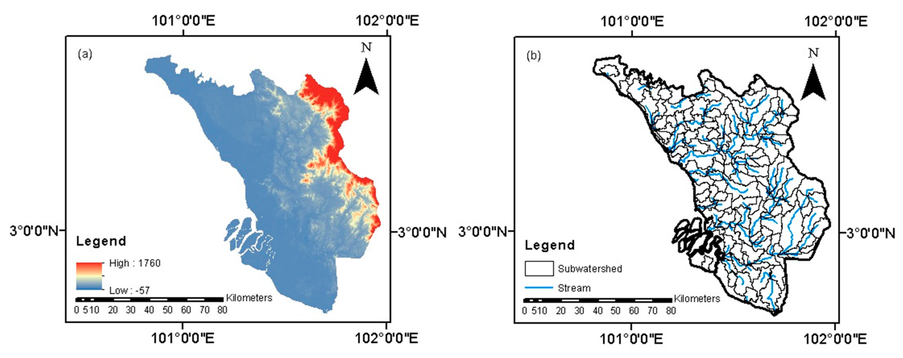
Selangor consists of mainly lowland dipterocarp forests (LDF) which is the major forest type in Malaysia and are taller than any other broad-leaved tropical rainforest in the world. On the shorelines and riverbanks of Selangor, mangrove forests can be found. The state of Selangor has six main rivers of which the Selangor River is the largest, with a catchment area of about 1960 km² covering about 25% of the state. The Selangor River runs from the upstream at Kuala Kubu Bharu in the east, near the Titiwangsa Mountains, to the Straits of Malacca at the downstream at Kuala Selangor in the west. The other major river is the Klang River that is 120 km long, with 11 major tributaries and a catchment area of 1288 km². It flows through Kuala Lumpur and ends up in the Straits of Malacca. Thus Selangor comprises three major river basins, namely the Klang, Langat and, most importantly, the Selangor river basin.
2.2. Data Collection and Geospatial Modelling
Global Multi-resolution Terrain Elevation Data 2010 (GMTED2010)-type DEMs were used for the study [19]. The DEM with a spatial resolution of 75 m was processed in ArcGIS to determine and extract hydrological parameters such as slope, flow direction, flow accumulation, drainage features and to delineate the watersheds. Figure 2 shows the DEM and the catchments and drainage features of Selangor, respectively. Considering the size of Selangor, the DEM with a pixel size (75 × 75m) was sufficient for the coverage of the multiple watersheds of the study area.
2.2.1. Hydrologic Soil Group Classification
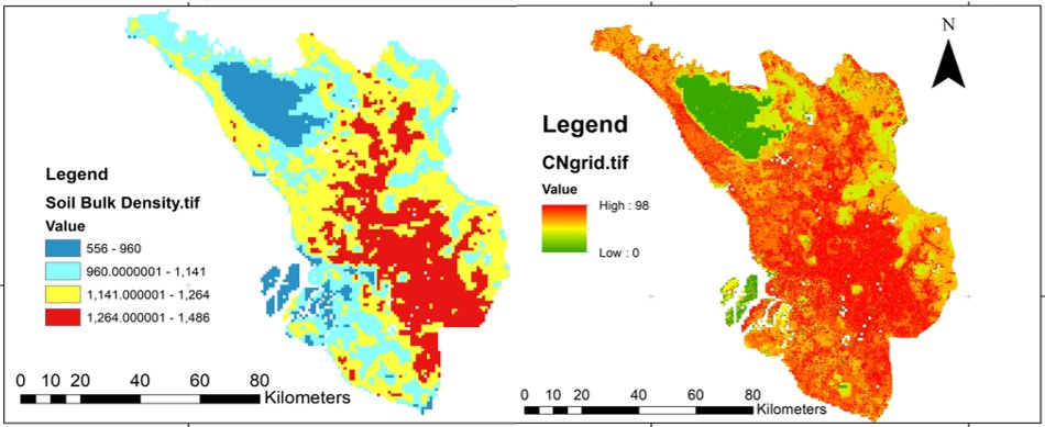
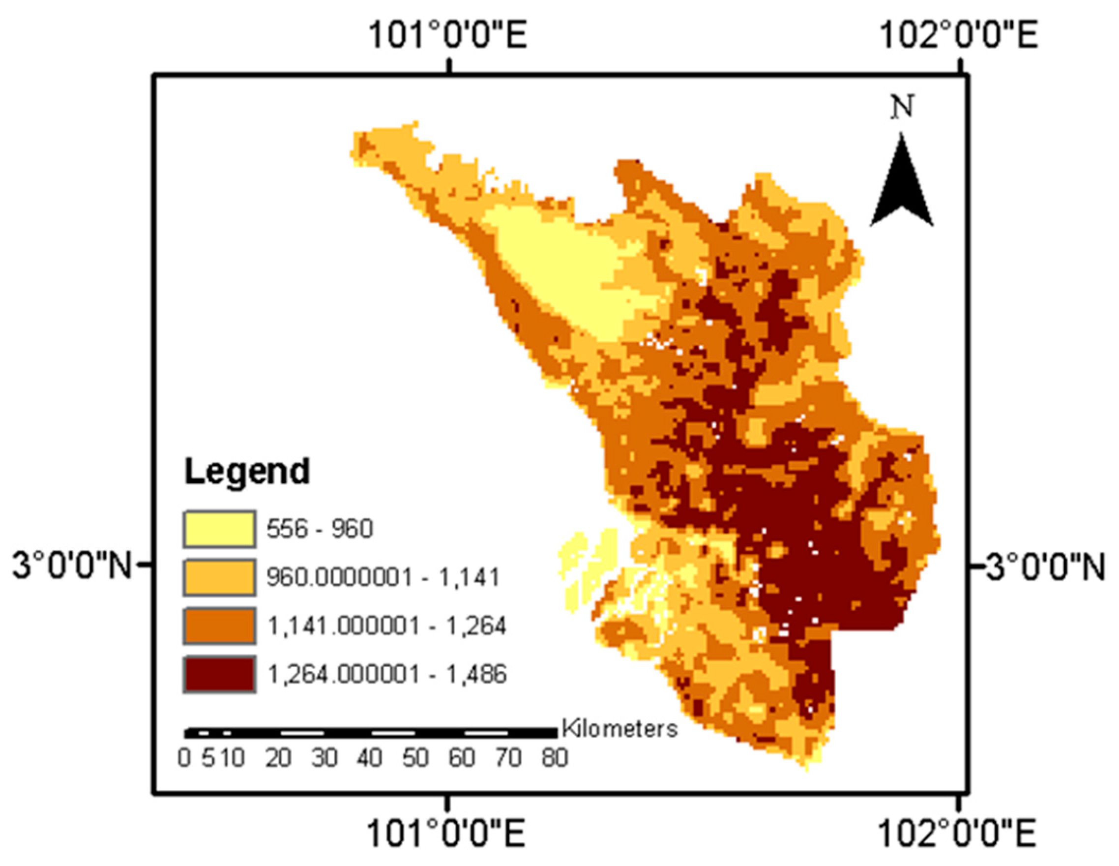
Soils play an important role in determining CN, with different soil types having different infiltration rates which are a function of surface intake rates and subsurface permeability. In developing the CN, the United States Department of Agriculture (USDA) utilized soil type data to derive the infiltration rate and categorized the soil based on the infiltration rate. In this study, soil data for Selangor was downloaded from SoilGrids [20] and further processed for soil bulk density. Thus, the bulk density of the soil was used in place of the infiltration rate. Soil bulk density is an important factor that affects soil infiltration capacity. As soil bulk density increases, soil porosity decreases, resulting in a decrease in soil infiltration capacity [21]. By having the bulk density data, the soil type is no longer significant. Figure 3 shows the processed soil bulk density of Selangor at 1m depth classified into 4 hydrologic soil groups (A, B, C and D). The details of the hydrological soil group classification are presented in Table 1.
2.2.2. Combination of Hydrologic Soil Group and Land-Use Classes
The latest land use for Selangor was developed from Landsat Operational Land Imager images of the year 2016 downloaded from the United State Geological Services (USGS) website. The Landsat images were mosaicked to improve coverage over the study area. A pan-sharpening operation was conducted to improve the spatial resolution of the multispectral visible bands to 15 m using the panchromatic band. The Selangor land use was classified into six different classes based on a supervised classification using the ArcGIS image analysis tool. The land-use classification (Figure 4a) includes water bodies, residential, industrial and commercial areas, plantations, green open spaces and forests. The land-use classification was then combined with the hydrologic soil group classification (Figure 3) to process and determine the CN using a relationship between hydrologic soil group and land cover as described in Table 2. Figure 4b shows the output map of the generated soil conservation service curve number.
2.2.3. Spatial Rainfall Data Processing
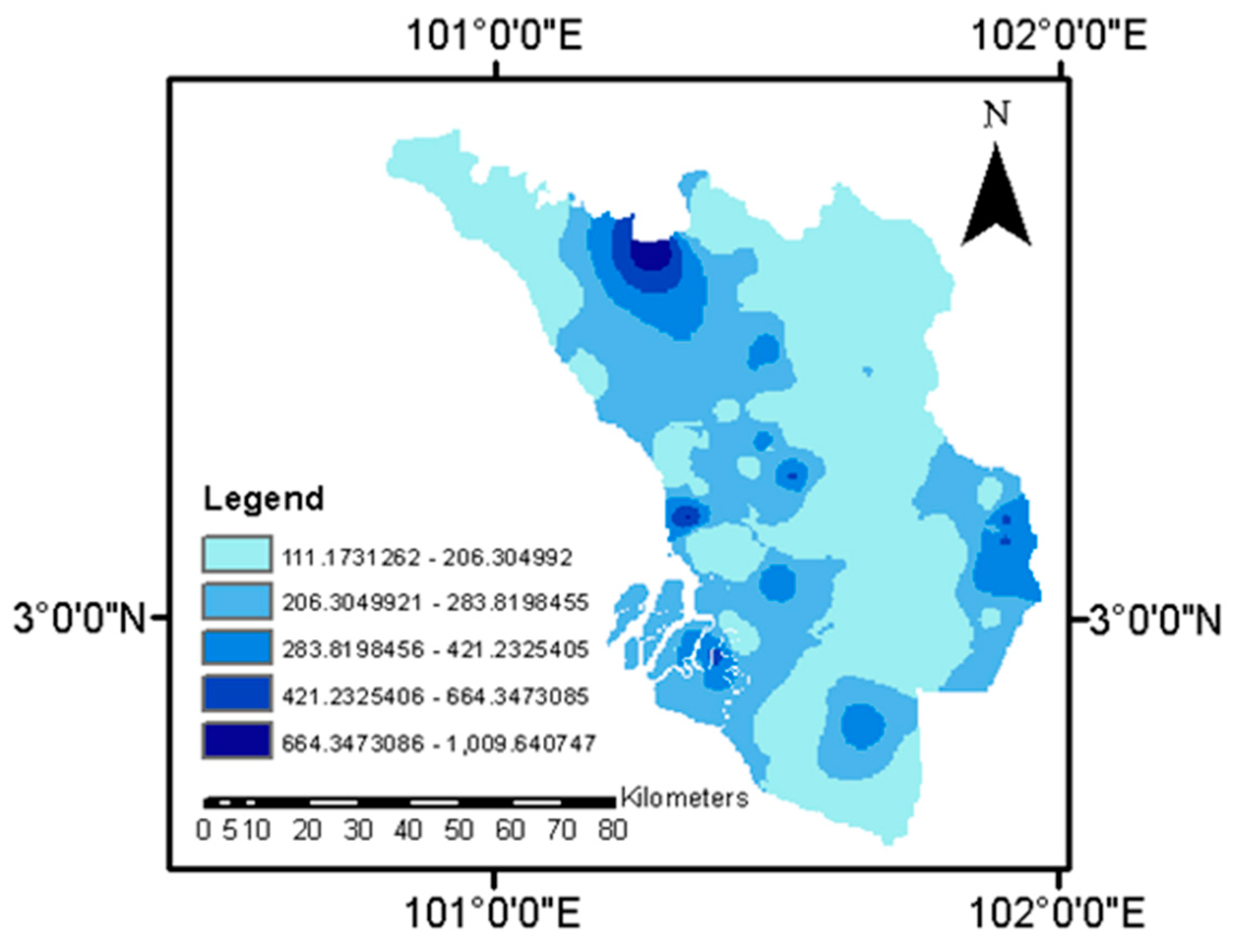
The daily rainfall data can be obtained from rainfall gauge stations throughout Selangor. For the study, rainfall data of 50 years from 1965 to 2015 were obtained from the Department of Irrigation and Drainage Malaysia (DID). Data from each rainfall station were checked and filtered for consistency. Stations with missing data were not taken into consideration. The mean maximum daily rainfall of each station was then spatially interpolated based on the inverse distance weighting (IDW) method using ArcGIS. Figure 5 shows the results of the maximum daily precipitation of Selangor.
2.3. Hydrological Modelling
2.3.1. Calculation of Curve Number Peak Discharge
The storm has to overcome a threshold determined by depression storage, interception as well as infiltration volume before runoff can occur. Initial abstraction is the amount of rainfall required to satisfy the aforementioned volumes. After runoff begins, additional losses due to infiltration will still occur. In general, accumulated infiltration increases with increasing rainfall up to certain maximum retention, and runoff also increases as rainfall increases. The ratio of actual retention to maximum retention is assumed to be equal to the ratio of direct runoff to rainfall minus initial abstraction. This can be expressed mathematically as [15].
where,
- F = Actual retention after runoff begins, mm
- S = Watershed storage, mm
- Q = Actual direct runoff, mm
- P = Total rainfall, mm
- I = Initial abstraction, mm
The initial abstraction should take into consideration of depression storage, interception and infiltration occurring prior to runoff. The relationship between I and S was estimated by analysing rainfall-runoff data for many small watersheds to eliminate the necessity of estimating both parameters I and S in the above equation. The empirical relationship is given by [22].
Substituting Equation (3) into Equation (2) gives:
The equation now has only two unknowns, one variable P and one parameter, S. S is related to curve number (CN) by:
where,
- CN = Curve number (From Table 2)
Finally, Equation (5) was combined with the spatially distributed parameters of rainfall, soil and land–use to simulate the runoff in the watersheds. The total daily discharge was computed by the following equation:
where,
- QCN = Total daily runoff discharge of the watershed, m3
- Qi = The depth of daily direct runoff of cell No. i, m
- Ai = The area of corresponding cell No. i, m2
- n = Total cell numbers of the watershed
2.3.2. Simulation of Unit Hydrograph Peak Discharge
The Clark-unit hydrograph model in Hydrological Engineering Center-Hydrological Modeling System (HEC-HMS) was specifically chosen for peak flow based on the Malaysian Hydrological Procedure (HP) No. 27, published by the Department of Irrigation and Drainage [23]. The HP No. 27 proposes empirical equations for both the storage coefficient R and the time of concentration Tc. For simplicity and consistency, the catchment area, stream slope, and main stream length are used to estimate Tc and R for this procedure.
where,
- A = Catchment area [km2]
- L = Main stream length [km]
- S = Weighted slope of main stream [m/km]
The weighted slope of main stream, S is given by the equation:
where,
- li = Incremental stream length
- Si = Incremental slope
The catchment area, main stream length and weighted slope of main stream is modelled in ArcGIS using the above stated methods. The design baseflow, QB of each stream is then calculated with the equation from HP No. 27:
where,
- A = Catchment area [km2]
The catchment area, A; precipitation, P; storage coefficient, R; time of concentration, Tc; design baseflow, QB were then inputted into HEC-HMS to model the peak discharge, QClark that will serve as a comparison against the ArcGIS-modelled peak discharge.
The Clark-unit hydrograph method was used as the control variable of the study. The curve number derived peak discharge was compared against the Clark-unit hydrograph peak discharge. The Clark-unit hydrograph rainfall-runoff relationships are derived based on average conditions and should be only used for design purposes. The same applies to the Tc and R values derived. The areal variability of catchment rainfall during a storm causes the time of concentration of a catchment to vary from storm to storm. This makes the assumption of uniform areal distribution of design storm invalid. Some unaccounted for storage depression (e.g., wetland, extremely flat catchment slopes) could lead to the overestimation of the peak discharge and the underestimation of the time to peak when using the equations [23].
3. Results
3.1. Peak Flood Discharge Estimation
It was observed in Figure 6a that the two peak discharges agree with each other fairly well, showing a linear regression of 0.76. The peak discharge derived from the CN method was an underestimation when compared to the Clark-Unit hydrograph peak discharge. The Clark-unit hydrograph is a lumped model that includes a lot of assumptions about hydrological processes. Because of these assumptions, lumped models have a tendency to over-or underestimate runoff values [24]. Hence, using the equation of the best fit line that intercepts the origin, a correction factor was applied to the peak discharge modelled after the CN method to calibrate it.
The graph of urbanized area of a watershed was plotted against the total curve number of a watershed. This was done to establish a positive relationship between urban area per watershed, Au (km2) and the sum of the curve number per watershed, CN from Figure 6b, it was observed that the total curve number of the watershed increases as the urbanized area of a watershed increases. This strong correlation was further proven with the high linear regression of 0.7107. Hence, it can be concluded that an urbanized area increases the runoff potential of a watershed.
Having proven the hypothesis of a positive correlation between urbanized area and curve number, the relationship between the calibrated peak discharge (Qpeak) and Curve Number (CN), precipitation (P) and watershed area (Aw) was investigated to formulate Equation (12) based on the three factors. This was successfully done by obtaining the regression coefficients between peak discharge and CN, P, Aw.
By plotting the corrected peak discharge against the curve number, watershed area and precipitation, it can be seen that the curve number and watershed area are relatively more correlated to the peak discharge than the precipitation. This can be explained as the peak discharge being directly related to the surface runoff of the watershed. Thus, the larger the watershed, the more surface area that is able to intercept rainfall and contribute to the peak discharge. In the case of CN number, it was concluded that the urban area increases the runoff potential of the watershed. Precipitation, however, showed a weaker correlation because the individual watersheds have different characteristics, stream lengths, and base flows. Base flow forms the initial input baseline parameter for runoff simulations, as there will usually be stream discharge regardless of the existence of rainfall. Runoff occurs when there is rainfall, thus, precipitation was considered in the development of the equation.
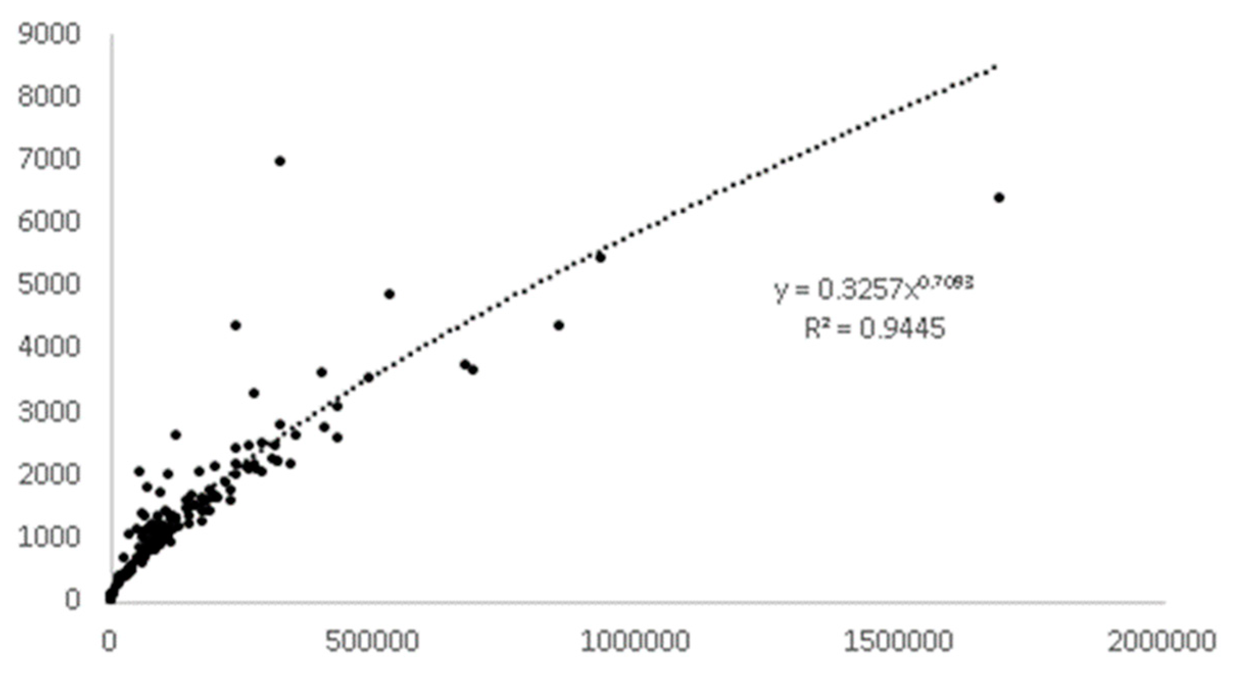
By taking the linear regression coefficient as the exponent of the respective factors, the multiplication product of the three powered factors was plotted against the calibrated CN modelled peak discharge. From Figure 7 below, it can be observed that the plotted best-fit power line has a strong correlation, with a regression coefficient of 0.9445. Hence, this power best-fit line is taken as the product equation.
3.2. Classification of Developed Model
A runoff model is defined by [25] as a set of equations that aid in the estimation of the amount of rainfall that turns into a runoff as a function of various parameters used to describe the watershed. According to [26], the runoff model, Equation (11), would be classified as an empirical model or more specifically, a regression equation. Regression equations find the functional relationship between inputs and outputs [25]. It is suggested by both [2] and [27] that empirical models are black-box models, meaning very little is known about the internal processes that control how runoff results are determined.
In terms of spatial structuring, according to [26] this developed model would be classified as a lumped model, as it treats the catchment area as a single homogeneous unit. In lumped models, the spatial variability of the catchment is disregarded [28,29]. Both the Clark-unit hydrograph and SNS-CN methods exhibit this property too. By assuming homogeneity over the catchment, the model loses the spectral resolution of the data. For example, rainfall and runoff patterns vary over space and time, but in lumped models, they are considered stationary [26].
3.3. Model Validation
Equation (12) was verified by plotting the estimated peak discharge against the peak discharge modelled with the curve number method. From Figure 8, it can be seen that the estimated peak discharge agrees fairly well with the calibrated CN modelled peak discharge, with a strong linear regression coefficient of 0.7854. Hence, the equation developed to estimate the peak discharge during a storm event that relates the watershed area, precipitation, and curve number can be considered as a valid equation.
The equation to estimate flood peak discharge taking into account the watershed area, precipitation, soil bulk density, and land use was successfully implemented. A higher resolution DEM and soil map should further improve the reliability of the curve number grid. The use of rainfall-runoff models was questioned by [30] as a better option for surface runoff modelling. Similar studies by [31] and [32] suggest that physically based models like MIKE-SHE (Système Hydrologique Européen) and TOPMODEL (TOPography based hydrological MODEL) have certain disadvantages as they require a large number of input parameters for calibration making their use highly data-dependent, time consuming and expensive. The approach presented in this study provides a straightforward method with limited parameter input to estimate peak discharges based on a GIS.
4. Conclusions
The hypothesis suggesting urbanization leads to increased runoff and short lag time of peak discharges holds true. In essence, the modelled peak discharge based on curve number was generally in agreement with the modelled peak discharge based on the hydrologic procedure No. 27. The curve number method, however, underestimated the peak discharge when compared to the Clark-unit hydrograph. Hence, a correction factor was introduced to calibrate the curve number modelled peak discharges. All three factors (curve number, precipitation and watershed area) were found to be correlated to peak discharge. This result demonstrated that the geospatial modelled peak flood discharge was reliable and provided an alternative method of monitoring potential flood in multiple watersheds. Ideally speaking, modeling of spatial variation of runoff generation by the infiltration excess mechanism and the downslope infiltration of runoff onto unsaturated areas require high spatial data input and or field sampling. For data-limited and inaccessible regions of Malaysia and most parts of the world, this has been a limitation in estimating the runoff in various watersheds. This proposed method applied geospatial techniques in the modeling of watershed area, land use, soil bulk density, spatial interpolated rainfall and runoff curve number and the derivation of the equation for estimation of peak discharge. The model serves as an alternative for estimation of peak discharge in watersheds and areas with poor data availability.
Author Contributions
R.C. and L.B. conceived, designed and performed the experiments; they analyzed the data and wrote the paper with contribution from A.C. and F.Y.T., and B.P. and A.M.A. professionally revised and edited the manuscript. The manuscript was discussed and reviewed by all of authors as they enhanced the context with sufficient references.
Funding
The research is supported by the Centre for Advanced Modelling and Geospatial Information Systems (CAMGIS), University of Technology Sydney under grant numbers: 323930, 321740.2232335; 321740.2232424 and 321740.2232357. This research was also supported by Researchers Supporting Project number RSP-2019 / 14, King Saud University, Riyadh, Saudi Arabia.
Acknowledgments
This research was supported by the University of Nottingham Malaysia Campus common project funds and learning resources. The metrological data were made available by the Department of Irrigation and Drainage (DID) Malaysia.
Conflicts of Interest
The authors declare no conflict of interest.
References
- Bashar, K.E.; Mutua, F.; Mulungu, D.M.M.; Deksyos, T.; Shamesldin, A. Appraisal Study to Select Suitable Rainfall-Runoff Model(s) for the Nile River Basin. In Proceedings of the International Conference of UNESCO Flanders Fust Friend/Nile Project, Sheikh, Egypt, 12–14 November 2005. [Google Scholar]
- Beven, K.J. Rainfall-Runoff Modelling: The Primer, 2nd ed.; Wiley-Blackwell: Oxford, UK, 2012. [Google Scholar]
- Xu, C.Y. Hydrologic Models; Uppsala University Department of Earth Sciences Hydrology: Sweden, 2002; Volume 2. [Google Scholar]
- Chow, V.T.; Maidment, D.R.; Mays, L.W. Applied Hydrology; McGraw-Hill Book Company: New York, NY, USA, 1988. [Google Scholar]
- Clark, C.O. Storage and the Unit Hydrograph. Proc. Am. Soc. Civ. Eng. 1945, 69, 1333–1360. [Google Scholar]
- Department of Irrigation and Drainage Malaysia. Urban Stormwater Management Manual for Malaysia; Department of Irrigation and Drainage Malaysia: Kuala Lumpur, Malaysia, 2012. [Google Scholar]
- Kokkonen, T.; Koivusala, H.; Karvonen, T. A Semi-Distributed Approach to Rainfall-Runoff Modelling—A Case Study in a Snow Affected Catchment. Environ. Model. Softw. 2001, 16, 481–493. [Google Scholar] [CrossRef]
- Maidment, D.R. Grid-Based Computation of Runoff. A Preliminary Assessment; Hydrologic Engineering Center, US Army Corps of Engineers: Davis, CA, USA, 1992. [Google Scholar]
- Ficklin, D.; Zhang, M. A Comparison of the Curve Number and Green-Ampt Models in an Agricultural Watershed. Trans. ASABE 2013, 56, 61–69. [Google Scholar] [CrossRef]
- Randolph, J. Environmental Land Use Planning and Management; Island Press: Washington, DC, USA, 2004. [Google Scholar]
- Arwa, D.O. GIS Based Rainfall Runoff Model for the Turasha Sub Catchment Kenya. Master’s Thesis, International Institute for Aerospace Survey and Earth Sciences, Enschede, The Netherlands, 2001. [Google Scholar]
- Mustafa, Y.M.; Amin, M.S.M.; Lee, T.S.; Shariff, A.R.M. Distributed Model for Changes in River Peak Flow due to Land Development. J. Inst. Eng. Malays. 2006, 67, 43–48. [Google Scholar]
- Khalid, N.F.; Din, A.H.M.; Omar, K.M.; Khanan, M.F.A.; Omar, A.H.; Hamid, A.I.A.; Pa’suya, M.F. Open-source Digital Elevation Model (DEMs) Evaluation with GPS and LiDAR Data. Int. Arch. Photogramm. Remote Sens. Spat. Inf. Sci. 2016, 42, 299–306. [Google Scholar] [CrossRef]
- Viney, N.R.; Vaze, J.; Chiew, F.H.S.; Perraud, J.; Post, D.A.; Teng, J. Comparison of Multi-Model and Multi-Donor Ensembles for Regionalization of Runoff Generation using Five Lumped Rainfall-Runoff Models. In Proceedings of the 18th World IMACS Congress and MODSIM09 International Congress on Modelling and Simulations, Cairns, Australia, 13 July 2009; pp. 3428–3434. [Google Scholar]
- United States Department of Agriculture. National Engineering Handbook; Part 630 Hydrology, Chapter 10, 210-VI-NEH; United States Department of Agriculture: Washington, DC, USA, 2004. [Google Scholar]
- Wang, S.; Fu, B.J.; Gao, G.Y.; Yao, X.L.; Zhou, J. Soil Moisture and Evapotranspiration of Different Land Cover Types in the Loess Plateau, China. Hydrol. Earth Syst. Sci. 2012, 16, 2883–2892. [Google Scholar] [CrossRef]
- Axel, B.; Daniel, N.; Gerd, B. Effects of Climate and Land-Use Change on Storm Runoff generation: Present Knowledge and Modelling Capabilities. Hydrol. Process. 2002, 16, 509–529. [Google Scholar]
- Balamurugan, G. Sediment Balance and Delivery in a Humid Tropical Urban River Basin: The Kelang River, Malaysia. Catena 1991, 18, 271–287. [Google Scholar] [CrossRef]
- USGS Earth Explorer. Available online: https://earthexplorer.usgs.gov/ (accessed on 6 December 2017).
- Soil, G. SIRIC World Soil Information. Available online: https://soilgrids.org/ (accessed on 21 February 2018).
- Li, Z.; Wu, P.; Feng, H.; Zhao, X.; Huang, J.; Zhuang, W. Simulated Experiment on Effect of Soil Bulk Density on Soil Infiltration Capacity. Trans. Chin. Soc. Agric. Eng. 2009, 25, 40–45. [Google Scholar]
- Chinh, L.V.; Iseri, H.; Hiramatsu, K.; Harada, M. A GIS-based Distributed Parameter Model for Rainfall Runoff Calculation using Arc Hydro Tool and Curve Number Method for Chikugo River Basin in Japan. J. Fac. Agric. 2010, 55, 313–319. [Google Scholar]
- Department of Irrigation and Drainage Malaysia. Hydrological Procedure No. 27, Estimation of Design Flood Hydrograph Using Clark Method for Rural Catchments in Peninsular Malaysia; Department of Irrigation and Drainage Malaysia: Kuala Lumpur, Malaysia, 2010. [Google Scholar]
- UCAR. Runoff Modelling Concept; Runoff Processes: 2010. Available online: https://www.meted.ucar.edu/hydro/basic_int/runoff/navmenu.php?tab=1&page=1.0.0 (accessed on 5 January 2018).
- Devi, G.K.; Ganasri, B.P.; Dwarakish, G.S. A review on Hydrological Models. Aquat. Procedia 2015, 4, 1001–1007. [Google Scholar] [CrossRef]
- Sitterson, J.; Kinghted, C.; Parmar, R.; Wolfe, K.; Muche, M.; Avant, B. An Overview of Rainfall-Runoff Model Types; United States Environmental protection Agency: Washington, DC, USA, 2017. [Google Scholar]
- Rinseme, J.G. Comparison of Rainfall-Runoff Models for the Florentine Catchment. Bachelor’s Thesis, University of Tasmania, Tasmania, Australia, 2014. [Google Scholar]
- Moradkhani, H.; Sorooshian, S. General Review of Rainfall-Runoff Modelling: Model Calibration, Data Assimilation, and Uncertainty Analysis. In Hydrological Modelling and the Water Cycle: Coupling the Atmospheric and Hydrological Models; Soroshian, S., Hsu, K.L., Coppola, E., Tomssetti, B., Verdecchia, M., Visconti, G., Eds.; Springer: Berlin, Germany, 2008; Volume 63, pp. 12–35. [Google Scholar]
- Singh, V.P. Computer Models of Watershed Hydrology Highlands Ranch; Water Resources Publications: Highlands Ranch, CO, USA, 1995. [Google Scholar]
- Matej, V.; Jana, V. GIS- Based Approach to Estimate Surface Runoff in Small Catchments: A Case Study. Quaest. Geogr. 2016, 35, 97–116. [Google Scholar]
- Nagarajan, M.; Basil, G. Remote Sensing and GIS-Based Runoff Modelling with the Effect of Land-Use Changes. Nat. Hazards 2014, 73, 2023–2039. [Google Scholar] [CrossRef]
- Costache, R.; Fontanine, I.; Corodescu, E. Assessment of Surface Runoff Depth Changes in Saratel River Basin, Romania, using GIS Techniques. Cent. Eur. J. Geosci. 2014, 6, 363–372. [Google Scholar]
Figure 1.
Location of Selangor in peninsular Malaysia.

Figure 2.
(a) Digital elevation model (DEM); and (b) catchment and drainage features of Selangor.

Figure 3.
Soil bulk density map.

Figure 4.
(a) Land-use classification of Selangor; (b) generated curve number map.

Figure 5.
Maximum daily precipitation of Selangor.

Figure 6.
(a) Graph of urbanized area per watershed against total curve number (CN); (b) graph of urbanized area per watershed against total CN.
Figure 6.
(a) Graph of urbanized area per watershed against total curve number (CN); (b) graph of urbanized area per watershed against total CN.

Figure 7.
Graph of calibrated CN peak discharge against the multiplication product of adjusted watershed area, precipitation and curve number.
Figure 7.
Graph of calibrated CN peak discharge against the multiplication product of adjusted watershed area, precipitation and curve number.

Figure 8.
Graph of CN modelled peak discharge against estimated peak discharge.


Table 1.
Hydrologic soil group classification.
| Soil Group | Infiltration Rate (mm/hr) | Bulk Density (kg/m3) |
|---|---|---|
| A | 8–12 | 555–960 |
| B | 4–8 | 960–1141 |
| C | 1–4 | 1141–1264 |
| D | 0–1 | 1264–1488 |
Table 2.
Runoff Curve Number.
| Description of Land Use | Hydrological Soil Group | |||
|---|---|---|---|---|
| A | B | C | D | |
| Cultivated land | 72 | 81 | 88 | 91 |
| Natural vegetation | 45 | 66 | 77 | 83 |
| Urban commercial | 77 | 85 | 90 | 92 |
| Urban housing | 61 | 75 | 83 | 87 |
| Bare land | 49 | 69 | 79 | 84 |
| Streets and roads | 98 | 98 | 98 | 98 |
| Open water | 0 | 0 | 0 | 0 |
© 2019 by the authors. Licensee MDPI, Basel, Switzerland. This article is an open access article distributed under the terms and conditions of the Creative Commons Attribution (CC BY) license (http://creativecommons.org/licenses/by/4.0/).
Share and Cite
MDPI and ACS Style
Cheah, R.; Billa, L.; Chan, A.; Teo, F.Y.; Pradhan, B.; Alamri, A.M. Geospatial Modelling of Watershed Peak Flood Discharge in Selangor, Malaysia. Water 2019, 11, 2490. https://doi.org/10.3390/w11122490
AMA Style
Cheah R, Billa L, Chan A, Teo FY, Pradhan B, Alamri AM. Geospatial Modelling of Watershed Peak Flood Discharge in Selangor, Malaysia. Water. 2019; 11(12):2490. https://doi.org/10.3390/w11122490
Chicago/Turabian StyleCheah, Ryan, Lawal Billa, Andy Chan, Fang Yenn Teo, Biswajeet Pradhan, and Abdullah M. Alamri. 2019. "Geospatial Modelling of Watershed Peak Flood Discharge in Selangor, Malaysia" Water 11, no. 12: 2490. https://doi.org/10.3390/w11122490
Note that from the first issue of 2016, this journal uses article numbers instead of page numbers. See further details here.