Permeability Coefficient of Low Permeable Soils as a Single-Variable Function of Soil Parameter

Faculty of Environmental, Geomatic and Energy Engineering, Kielce University of Technology, 25-314 Kielce, Poland
*
Author to whom correspondence should be addressed.
Water 2019, 11(12), 2500; https://doi.org/10.3390/w11122500
Submission received: 16 September 2019
/
Revised: 19 November 2019
/
Accepted: 22 November 2019
/
Published: 27 November 2019
(This article belongs to the Special Issue Modeling of Flow and Transport in Saturated and Unsaturated Porous Media)
Abstract
:Based on the results of experimental studies concerning the filtration coefficient, the Darcianity of the observed flows for eight cohesive soils at four hydraulic gradients was analyzed. It is observed that linear dependence of flow velocity on hydraulic gradient is an approximation only, and it is the worse the more cohesive a given soil is. Despite this, Darcy’s law can be a correct approximation of the empirical relationship between hydraulic gradient and the flow velocity, also in very cohesive soils. A statistical analysis was carried out to identify correlation between soil properties and permeability coefficient. For each soil, 109 parameters were analyzed, among others applying mercury intrusion porosimetry, scanning electron microscopy, dynamic image analysis, and laser diffraction. Ultimately, three single-variable models best fitted to the experimental data were found, using the plasticity index IP as the independent variable, the average pore diameter DP, and the convexity of silt fraction particles. All model parameters are statistically significant at p < 0.05. Comparison with reference multi-variable models showed that the best fit for experimental data is observed by the model with the plasticity index, while the results suggest low usability of single-variable models with structural parameters.
1. Introduction
Increasing interest in cohesive soils and clay minerals has been observed in recent years on the part of environmental engineering. Soils of this type show a tendency for particles to stick to each other due to intermolecular interactions and, as a result, they usually have low permeability. This is due to the properties of these materials, allowing use of them, among others, as pollution sorbents and mineral insulating barriers at landfills, including those used for radioactive waste. Any soil which is to be used as a barrier needs to have low permeability, self-sealing capability, and high cation exchange capacity [1,2]; hence, thorough examination of the mentioned parameters is crucial. Insufficient or even incorrect testing of soils in this regard may result in underground water contamination with various substances coming from municipal and industrial wastes stored in landfills. For example, in the case of industrial waste storage (acidic waste water), underground water protection is implemented using clay minerals, which are required in order to reduce hydraulic conductivity of clays occurring naturally beneath landfills [1]. Cohesive soils and clay minerals are also used in urban solid waste storage facilities and mine waste dumps as barriers and sealings [3]. They also work as geological reservoirs used to store carbon dioxide [4]. At the same time, bentonites are used to store radioactive and other hazardous waste because they have proved to have special expansive properties and high water adsorption potential [3,5,6,7]. Moreover, they are used to eliminate toxic chemical compounds from environment when reducing the extent of pollution dispersion in soil, water, and air [6,8]. Bentonites are also used in the production of impermeable geosynthetic mats and geomembranes resistant to aggressive chemical agents [9].
Erroneous analysis of factors determining soil permeability may involve serious consequences because a disadvantageous effect of filtration is manifested by the loss of soil medium stability. These phenomena may include: suffusion (washing of mineral particles), quicksand (soil liquefaction), hydraulic penetration, or replacement. Negative impact of the filtration forces on soil is observed, for example, in the vicinity of flood banks when water level is high in rivers (most often at the foot of landside slope and drainage facilities), and while making constructional foundation trenches (there is the risk involving the loss of soil stability in riverbed and slopes). These areas of disturbed balance due to water migration and their further uncontrolled growth may be the reason for various breakdowns [10]. Stringent requirements resulting from the need to protect environment entail greater interest in adequate evaluation of geotechnical parameters, including permeability coefficient [11]. Regarding mentioned environmental engineering problems, it is extremely important to know geotechnical parameters and mechanisms determining soil permeability [12,13,14].
However, while one can find many empirical equations useful in estimating the value of permeability coefficient for coarse soils or sediments (sands and gravels), solutions applicable to poorly permeable soils are significantly rarer. Some of these “coarse” formulas are attempted to be used in cohesive soils (especially the so called Kozeny-Carman formula introduced in first half of 20th century [15]), but, as not taking into account the water-mineral interactions manifesting as the soil plasticity, all of them seem less useful in such a context. There are presented a number of empirical formulas used to calculate the permeability coefficient for different soil types on the basis of their selected parameters [16,17,18,19,20]. However, these empirical or semi-empirical models were introduced without any statistical treatment, and it is not clear how high absolute and relative mean errors can be expected and if the estimates of model parameters are statistically significant. In other words, it is hard to assess their predictive capacity in terms of modern statistics.
This study presents an attempt to find empirical single-variable models on the basis of the results of owned permeability coefficient measurements on samples of eight poorly permeable soils, which differ considerably in their mineralogical composition, origin, and physical and structural properties. The search for the models was carried out without making any presumptions regarding lesser or greater usability of a given parameter, meaning that all 109 analyzed parameters constituted equivalent input data. Soil parameters were divided into two groups: physical parameters and structural parameters, the latter requiring more refined experimental techniques, such as mercury intrusion porosimetry (MIP), scanning electron microscopy (SEM), dynamic image analysis (DIA), and laser diffraction method (LD). According to the initial hypothesis, models based on structural parameters may prove to be more perfect, although physical parameters, such as the plasticity index and the Atterberg limits, may include more information on the clay-water interaction and are more easily accessible as no specialized equipment needs to be used to determine them.
However, an attempt to search for models with the number of soil parameter limited to one has an essential theoretical meaning, allowing for a strict identification of soil properties most responsible for the flow phenomena in clay-water systems.
2. Materials and Methods
2.1. Materials
Eight cohesive soils were subject to experiments, numbered from 1 to 8 for the identification purposes. The soils were collected in Poland in the region of Swietokrzyskie Mountains. Pursuant to Polish standard [21]/European standard [22], they were named as follows: soil 1—loamy sand/silty sand-siSa, soil 2—sandy clay/silty sand-clSa, soil 3—clay/clay-Cl, soil 4—loam/silty clay-saclSi, soil 5—clay/clay-Cl, soil 6—firm silty clay/clay loam-sasiCl, soil 7—clay/clay-Cl-siSa, and soil 8—silt/sandy silt-saSi. Basic characteristics of the soils are presented in Table 1, while selected structural properties are given in Table 2.
2.2. Methodology
2.2.1. Experimental Method and the Test Stand
In addition to the tests mentioned in Table 1, mineralogical composition of the soils was determined by the XRD method using an EMPYREAN X-ray diffractometer from PANalytical.
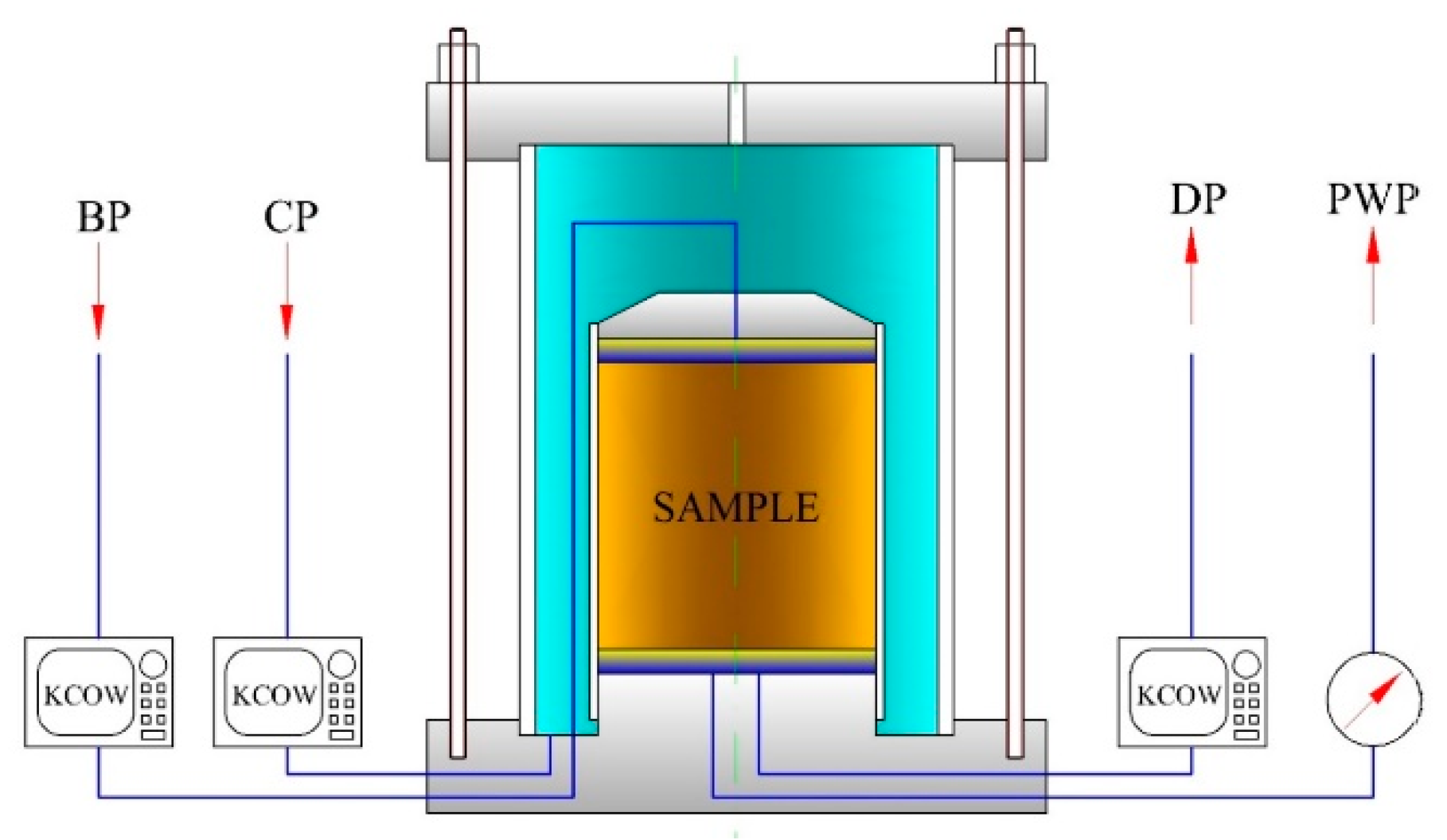
The degree of pore saturation with water is one of significant factors affecting the soil water permeability. The elimination of this factor impact is related to performance of tests in apparatus, which enables carrying out the experiments under total saturation conditions [23]. Because of that, the permeability coefficient in this study was determined in a triaxial compression chamber, in accordance with the Head’s methodology (for the first time published in 1982) [24,25] and standards found in [26,27,28,29]. Triaxial compression apparatus is considered a very precise device, which is confirmed in the literature, e.g., see [30]. The apparatus consists of three water volume and pressure controllers, the chamber of triaxial compression apparatus (maximum pressure of 1700 kPa), frame with load up to 50 kN, an MPX 3000 miniscanner, collecting information from sensors, and a control computer with specialized software VJ Clisp Studio by the VJ Tech company. The diagram of testing instruments is presented in Figure 1.
2.2.2. Sample Preparation
Samples were formed artificially by compaction in the Proctor apparatus at previously set moisture content. Then rollers 38 mm in diameter were obtained by means of the Shelby cylinders. After macroscopic assessment of the core quality, the least disturbed segment was selected and then a sample of 76 mm in height was cut from it. Samples prepared in this way were placed in a rubber membrane on the base and were covered from the top with a small dome. A flexible shield covering the sample was pressed to the base and the dome by four sealing O-rings. Moreover, porous stones with a permeability coefficient at least 10 times higher than that of the tested sample were placed between the sample and the aforementioned elements [29]. The chamber was put on the sample prepared in such a way, which was next filled with deaerated water, that enabled applying isotropic stresses. The application of various hydraulic pressures to the top and bottom part of the sample through the dome and base resulted in formation of a hydraulic gradient.
2.2.3. Test Procedure
The applied procedure comprised three stages: saturation, consolidation, and filtration. Stage one, i.e., saturation, was carried out in two phases:
- phase I—application of a small hydrostatic pressure to the lower base of the sample, so-called flushing, and
- phase II—pumping deaerated water to the sample via a closed system connected to the sample’s bottom and top, in a so-called method with the use of two back pressures.
At this stage of testing the pressure in the triaxial chamber and the back pressure were increased in such a way that the isotropic effective stress in the sample would remain on a constant level during the entire saturation procedure. An increment of 100 kPa was used, and the amount of this stress was chosen so as to prevent radial swelling of the soil. Experiments show that, for the studied soils, a sufficient stress amounted to 10 kPa (i.e., a stress slightly higher than the swelling pressure was applied). During the saturation, the sample’s height was observed the entire time.
The state of studied soil saturation under conditions of impossible lateral expansion was estimated based on the value of Skempton parameter B [31], determined from formula [24,27,28]:
where: B: Skempton parameter (-); Δu: change of water pressure in pores (kPa), and Δσ: change of pressure in the chamber (kPa).
Because the parameter B is dependent on soil properties, the saturation process is different in different soils. In general, the state of full saturation is assumed for the parameter value B = 1. However, for non-permeable soils (investigated soils), it is justified to assume the state of full saturation for parameter B ≥ 0.95. The time necessary to obtain such a value for each sample was approximately 2–3 days.
After the finished stage of saturation, the samples were isotropically consolidated to the value of effective stresses of approximately 50 kPa. Formulae given by Head [25] were used in calculations:
where
- σ′: required effective stress (kPa),
- σ: isotropic pressure in the chamber (kPa)—in the present study, this is a pressure equal to the last pressure applied in the saturation phase, i.e., 650 kPa—, and
- ū: mean pore pressure calculated based on the formulawhere
- ub: pressure at the sample’s top (back pressure) (kPa), and
- uc: pressure at the sample’s base (kPa).
At this stage, the excess of water pressure in pores, i.e., the difference between the final constant pressure of pore water and the back pressure from the last saturation step, was dispersed.
After completed consolidation, the third stage of the study, i.e., filtration, was started. A series of water-permeability coefficient measurements were performed using two back pressures, at various values of hydraulic gradient. To this end, pressure differences were used between the top and bottom base of the sample, ranging from 5 to 45 kPa, which corresponded to hydraulic gradients of 7, 10, 20, and 30. The values were chosen so as to make the obtained yields reliable. The permeability constant was determined for the top-down flow. Measurements were carried out at a constant temperature of 22 °C in an air-conditioned room. After the completion of the measurement series, all the results were exported to the Excel program to perform further calculations.
Knowing the flow, the set gradient, and the sample’s surface area and height, the water-permeability of soil was calculated based on the formula given below:
where
- k—permeability coefficient (m/s),
- Q—flow rate (m3/s), l—sample’s height (m),
- A—area of sample cross-section (m2), and
- Δh—difference of pressures at the sample’s top and bottom (m).
3. Results and Discussion
3.1. Raw Results
The tests of eight soils conducted using the triaxial testing apparatus allowed obtaining the values of permeability coefficients at four different hydraulic gradient values. The results are shown in Table 3.
3.2. Variance Analysis
The variance analysis was carried out using the Statistica 8 software in order to check whether the results for various soil types and hydraulic gradients i differ from each other in a statistically significant way. The analysis involved evaluating the independent effect and interactions of the factors soil and hydraulic gradient on the observed values of permeability coefficients k. The results are shown in Table 4.
The p-values shown in the Table 4 are the probability that different permeability coefficient k values (dependent variables) for various groups classified with classifying predictors (independent variables) have been obtained in a purely random way—that is as a result of difficult to assess experiment errors. In other words, it is the probability that the so-called null hypothesis is true. The null hypothesis is the statement that there is no difference among the groups, e.g., different soils have the same permeability coefficient, or else permeability coefficients obtained for various hydraulic gradients are equal. The value of 0.05 is usually assumed to be the boundary value of the probability p.
It can be seen from Table 4 that all p-values are few orders of magnitude smaller than 0.05, allowing rejection of the null hypothesis. In terms of the current experiments, it can be stated that both soil type and hydraulic gradient, as well as interaction of these two factors, significantly affect the obtained values of permeability coefficient k.
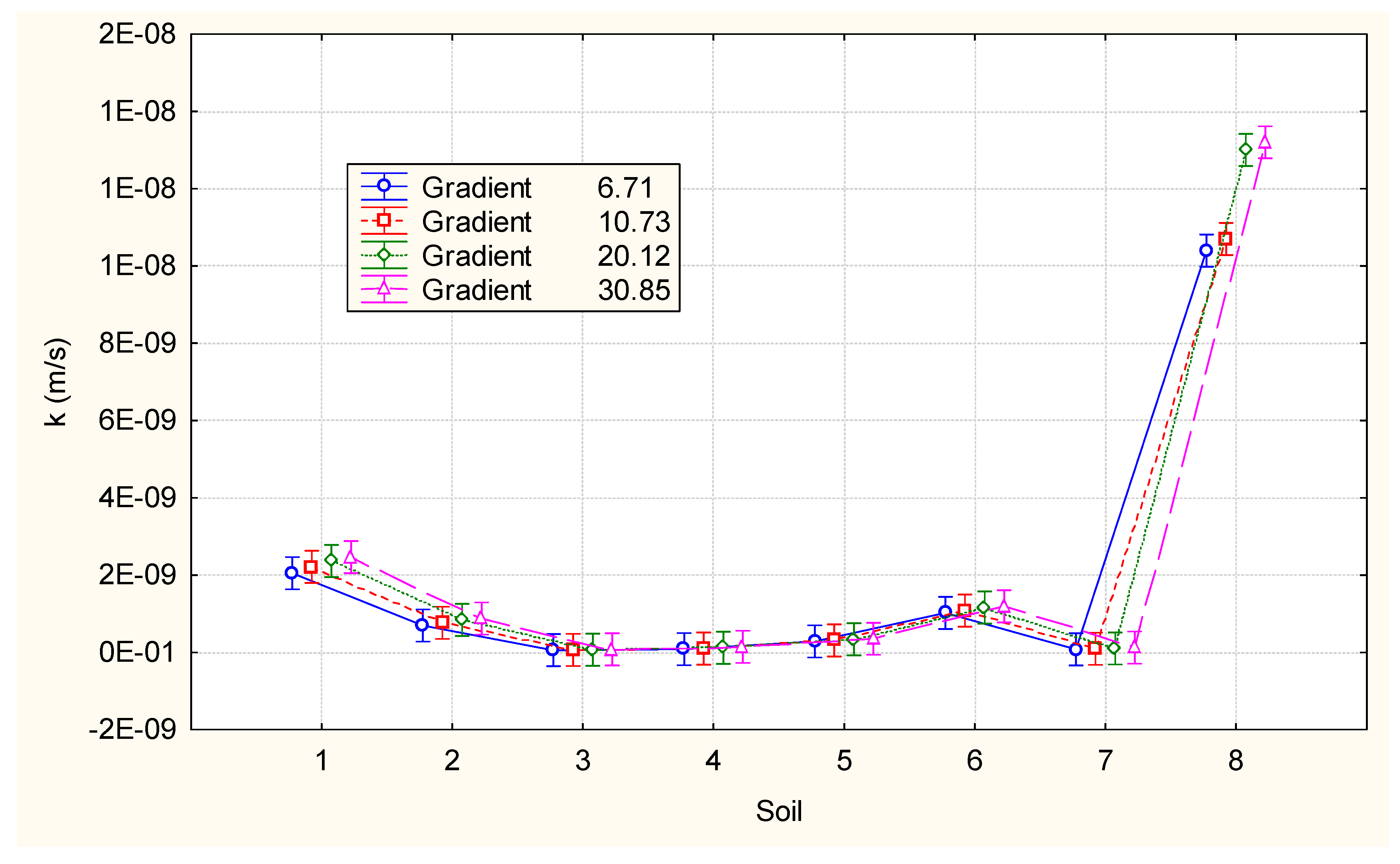
Partial η2 (that is the so-called effect size measure, η2 ∈ < 0; 1>) is an indicator determining which fraction of variability in range of variable A (dependent variable, in our case, k) is explained by variable B (independent variable, in our case, soil and hydraulic gradient). In other words, partial η2 explains which of the independent variables has greater effect on the results of the dependent variable. Data in Table 4 show that the type of soil has extremely large impact (partial η2 close to 1). The effect of hydraulic gradient i is considerably smaller, but it is still statistically significant. It means that empirical models characterizing the permeability coefficient and taking into account the sole hydraulic gradient i are reasonable. However, the effect of the gradient in interaction with soil is bigger than the effect of the sole gradient. This result is in agreement with intuition: The same gradient in soils of different structures must result in different hydraulic conductivity; in other words, more permeable soils strengthen the effect of the gradient and vice versa. Summarizing, the measured values of permeability coefficients depend on the soil type and, to a lesser degree, on the value of hydraulic gradient. An increasing relationship is observed in the latter case, which can be seen in Table 4, where mean values for each soil and the hydraulic gradient combination are gathered. The value of kmean represents “the mean of the means” value, i.e., the values of the permeability coefficient treated as being independent of the hydraulic gradient.
3.3. Darcianity of the Observed Flows
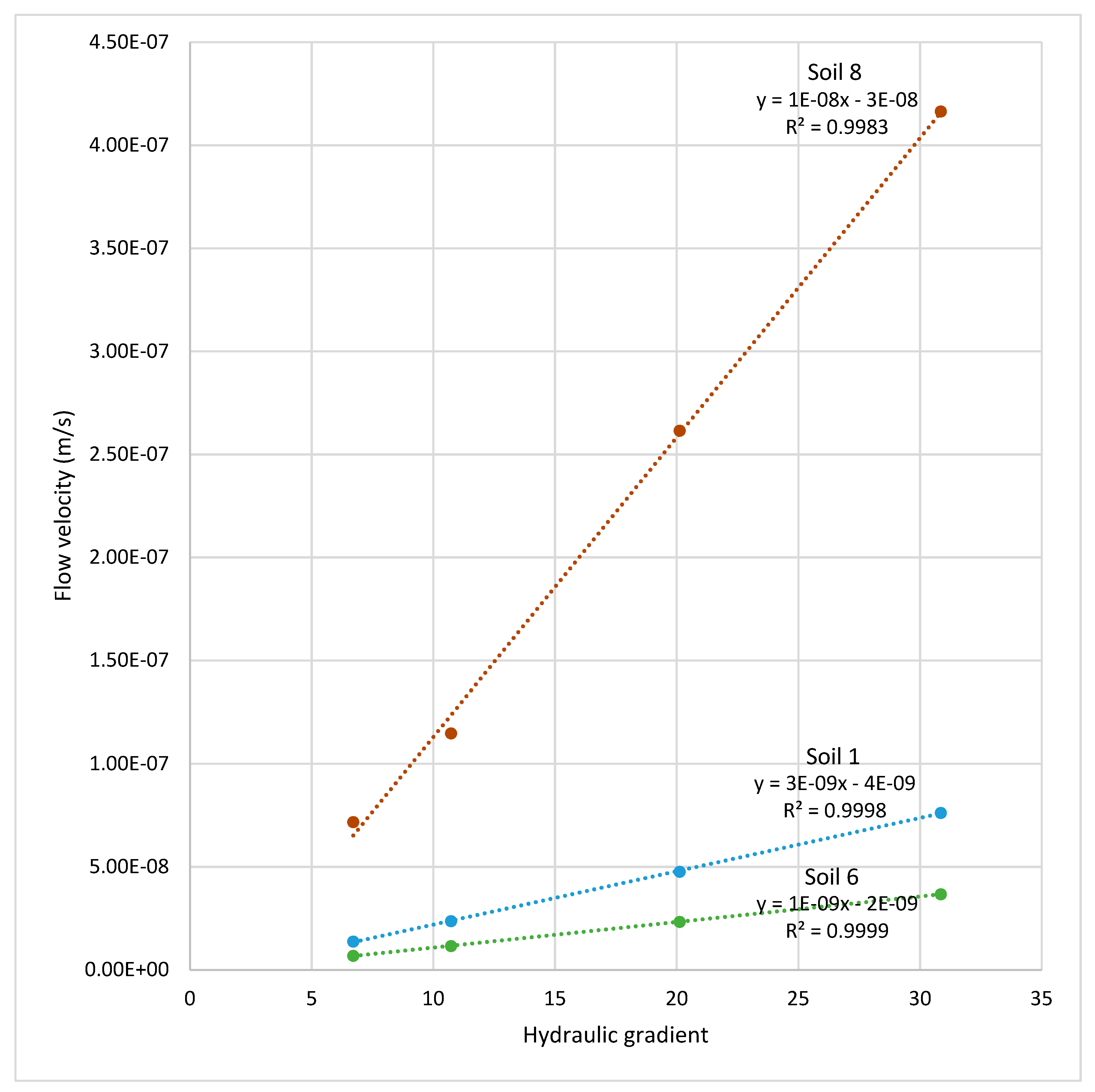
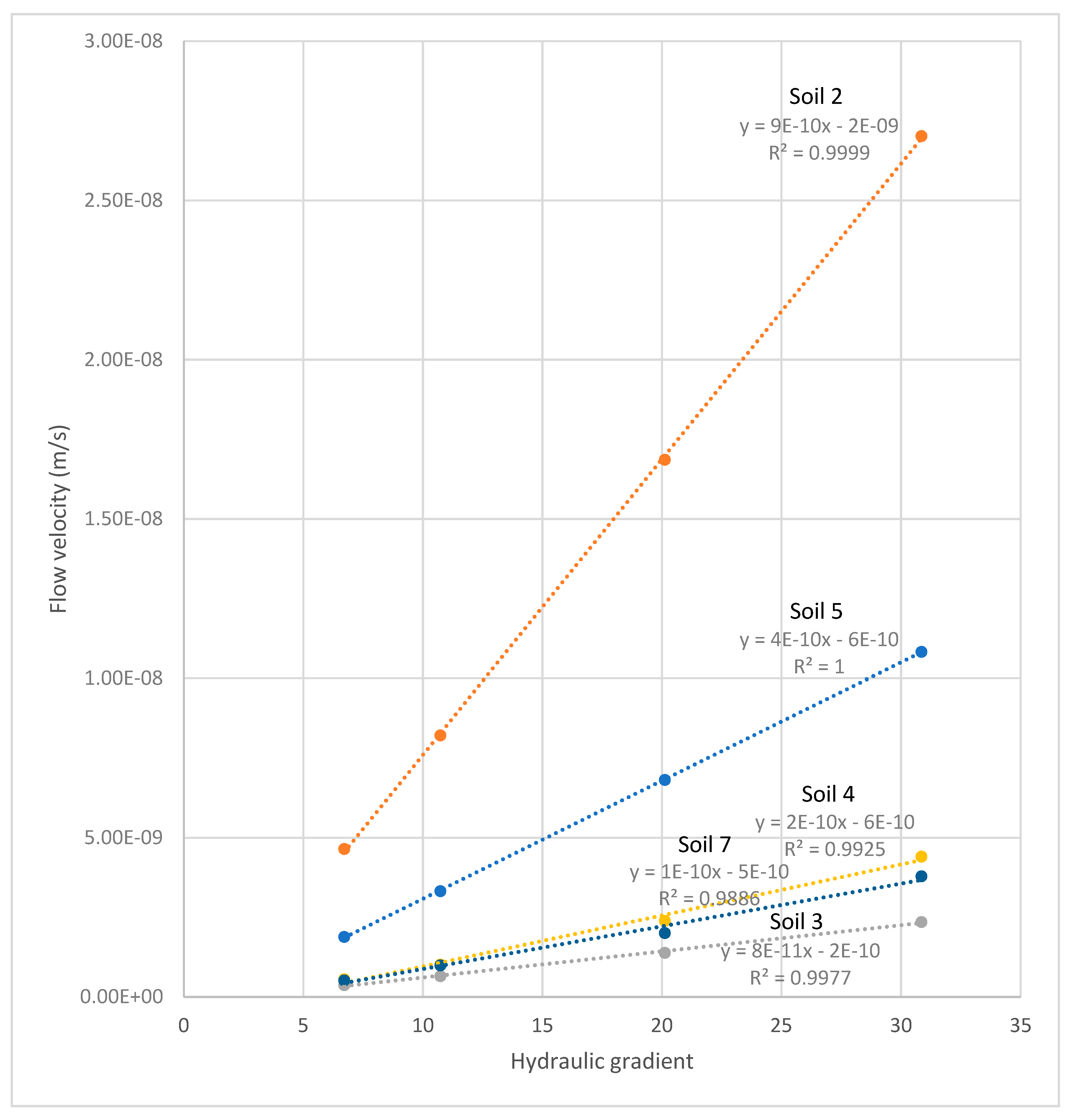
Data shown in Table 4 and in Figure 2 cannot be treated as settling the issue of Darcianity or non-Darcianity of the observed flows. Assuming linear relationship between the flow velocity and the hydraulic gradient as indicative for Darcian flow, we compared two regression models in the form V = f (i). For the pairs (ij, Vj), linear approximation and non-linear approximation using power, logarithmic, exponential, and second-order polynomial functions were performed. Among the nonlinear functions, the best fit was observed for the second degree polynomial (R2 = 1 in all cases). In Table 5 and in Figure 3 and Figure 4, fitting parameters of linear relationships are shown. These results show that the relationship V = f (i) is actually non-linear. It is particularly evident in soils no. 3, 4, and 7. The specificity of just these soils against the others consists in the highest values of the colloidal activity (1.23, 1.24, and 1.36, respectively). Moreover, soils no. 3 and 7 prove to have highest values of plasticity index Ip.
It can be concluded that linear dependence of velocity on hydraulic gradient is an approximation only, the worse the more cohesive a given soil is. However, as seen in Table 5 and in Figure 3 and Figure 4, even in the case of the worst fitting (soil no. 7), the linear function can be considered well fitted (R > 0.99427) and highly statistically significant (p < 0.00573). Hence, Darcy’s law is, from an engineering point of view, a correct approximation of the empirical relationship V = f (i), also in very cohesive soils.
3.4. Empirical Regression Models
In order to gain a preliminary insight into the data, the Statistica 8 software was used to create the correlation matrix of averaged permeability coefficient k values with 109 soil parameters, including: volumetric density of soil; volumetric density of soil skeleton; natural humidity; yield point (determined using the roll test and cone penetrometer methods); liquid limit (determined using the Casagrande, Vasiliev, and cone penetrometer methods); plasticity indexes; colloidal activity; organic matter content; pH value; the proportion of clay, silt, sand, and gravel fractions (measured using three methods: hydrometer, laser diffraction, and image analysis); reduced fractions calculated for hydrometer analysis; percentage of pores within ranges: <3 nm, 3–10 nm, >10 nm; total area of pores; pore size median—measured volumetrically; total mercury intrusion volume; average pore diameter; volumetric density of pores at the pressure of 3.65 kPa; porosity; void ratio (determined using the mercury porosimetry method or through calculations); minimum, maximum, and mean pore area and its medians; minimum, maximum, and mean pore circumference with median (the NIA Numerical Image Analysis method); shape factors: sphericity, convexity, and shape proportionality (determined using the image analysis method for silt and sand fraction, and mean value); total and outside specific surface; approximate montmorillonite content; two sorption moisture values: w50 and w95 (sorption test method); and specific surface determined relative to the volume and mass (laser diffraction and image analysis methods for all fractions and mean value).
For the majority of parameters, correlation coefficients (R) are: |R| < 0.5 (this value indicates poor correlation). Moderately strong correlations (0.5 < |R| < 0.7) of permeability coefficients were observed for the following parameters: liquid limits determined according to Casagrande and cone penetrometer methods (wLC, wLP), plasticity index (Ip = wLC − wpw), clay and silt fraction (fπ, fi′, fπ′—obtained using the hydrometer method), pore size median (Mp—the MIP method), minimum pore circumference (Omin—the NIA method), convexity of particles and particle shape proportionality coefficient for silt fraction (ψc2–50, ψa2–50—the DIA method), as well as sorption moisture w95, whereas strong correlation (|R| > 0.7) was observed for these parameters: average pore diameter (Dp—obtained using the MIP method), and convexity of particles for sand fraction (ψc50–2000—the DIA method).
The complete correlation matrix allowed initial selection of parameters best correlated with permeability coefficient k (|R| > 0.5), and those parameters, which were thought to be significant for filtration phenomenon. Relatively low values of correlation coefficient in the matrix could be resulting from strongly non-linear dependence for such parameters as the plasticity limit wpw, the colloidal activity IA, clay fraction content fi obtained using the hydrometer method, porosity and void ratio obtained using the MIP method (nHg, eHg) or through calculations (nobl, eobl).
The average pore diameter Dp is given by the following equation:
where
- V: pores volume, determined by the mercury intrusion porosimetry (MIP), and
- S: pores surface area, determined by the mercury intrusion porosimetry (MIP).
The values of correlation coefficients R for parameters selected in this way are shown in Table 6. The distinction between “physical” and “structural” parameters here partially is conventional in character and is partially based on the way in which individual parameters can be obtained. While the “structural” parameters require more refined techniques, the “physical” ones can be determined by use of traditional simple methods of soil science. However, the content of clay fraction, for example, is no less “structural” than pore diameter determined by use of Mercury Intrusion Porosimetry. On the other hand, models using structural parameters as difficult to obtain as the permeability coefficient itself seem less practical, though they could have theoretical significance in understanding the nature of the transport processes in porous media.
Then, the selected parameters were used to create empirical models characterizing permeability coefficient k. The Levenberg–Marquardt non-linear estimation method was applied for that purpose.
The empirical models were determined using the following functions:
- power:
- logarithmic:
- exponential:
where
- x: analyzed soil parameter, and
- a1, a2: estimators of model parameters.
The values of correlation coefficients R for the models are shown separately for physical and structural characteristics in Table 7 and Table 8. The highest values are printed in bold and red.
The correlation coefficient values allowed finding the best fitted models with one parameter for both of the above-mentioned groups of physical and structural parameters. According to Table 7, the highest values of the coefficient R are observed for the following parameters: Ip (R = 0.99499, power function), CF′ (R = 0.99238, power function), w95 (R = 0.98919, exponential function), wLC (R = 0.98679, exponential function), and SF′ (R = 0.97368, exponential function), whereas, according to Table 8—for Dp (R = 0.98752, power function)—, ψc2–50 (R = 0.98591, power function). Table 9 presents specified estimators of parameters a1, a2 for the best-fitted models with the corresponding statistical significance values and confidence intervals.
The models with structural parameters do not prove to be better fitted than the models with physical parameters. Presumably, this is the result of the effect of the “non-structural” factors, in particular capillarity and the bound water properties. They are strongly related to such physical parameters as the plasticity index, the clay fraction content, sorption moisture w95, and the colloidal activity. These facts allow an important general conclusion: it is not possible to effectively model the water flow in poorly permeable soils using structural data only, related with the volume, size, and shape of pores or particles.
The values of estimators statistically significant at p < 0.05 are printed in bold and red. Parameter estimators of the models with CF′, w95, wLC appear statistically insignificant at the 0.05 level. In turn, the model with silt fraction SF′ is characterized by the least correlation coefficient of all the models in Table 9. Taking into account the above, the following empirical model with one physical parameter is proposed:
where
- Ip: plasticity index calculated from Ip= wLC − wpw (%), and
- a1 = 1.48 × 10⁻⁶, a2 = −2.93561.
The following empirical models with one structural parameter are proposed:
where
- Dp: average pore diameter obtained using the MIP method (nm),
- a1 = 2.09 × 10⁻¹⁴, a2 = 1.85356,
or
where:
- ψc2–50: convexity of particles for silt fraction obtained using the DIA method (-), and
- a1 = 4.88 × 10⁻¹⁹, a2 = −2.04 × 10⁻².
3.5. Models Validation
Four common metrics were used in the validation process for measuring the differences between permeability coefficient values predicted by the proposed models and the values observed: Mean Absolute Error (MAE), Mean Bias Error (MBE), Mean Absolute Percentage Error (MAPE), and Root-Mean-Square Error (RMSE). The results are compared with results obtained by use of two frequently used models from references, among others, such as equation based on the void ratio e, plasticity limit wp, plasticity index Ip [17].
and, on the void ratio, the percentage of clay fraction fi, and the colloidal activity IA [18]:
The calculations using Equations (12) and (13) were done for three sets values of the void ratio, i.e., obtained by use of MIP (eHg) calculated from the dry density and the specific gravity (ecalc) and the void ratio in the saturated state (ecalc). In the cases of both equations, ecalc yielded the best fitting to experimental data, and these results are presented further by default.
In Table 10, values of the above listed metrics are presented for Equations (9)–(13).
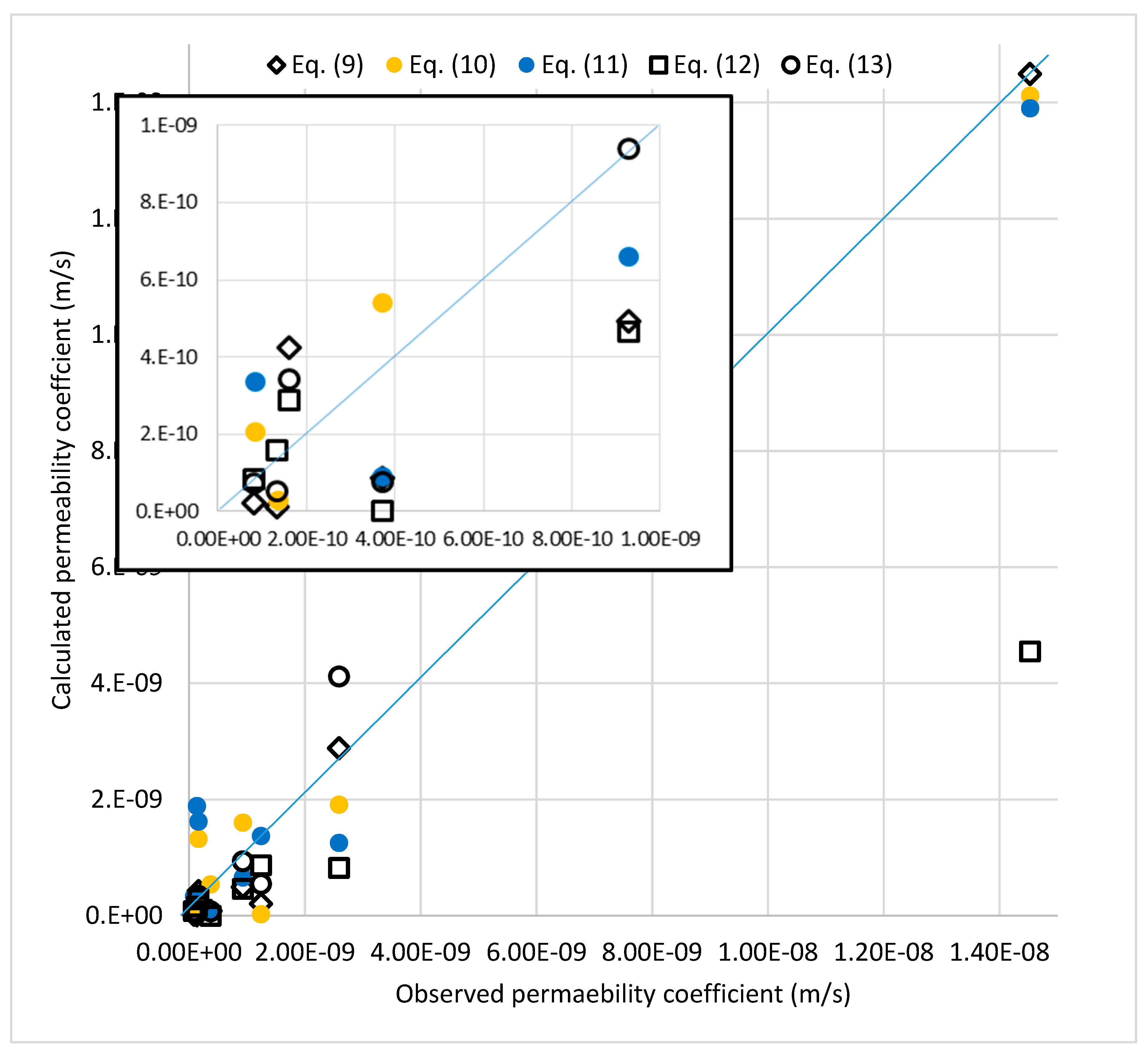
Figure 5 represents scatter plot for values observed and calculated using the five analyzed models. Data scattering for the three most impermeable soils with k < 1 × 10⁻⁹ m/s (nos. 2–5) is more conveniently presented in the inlay.
It is apparent from data shown in Table 10 and in Figure 5 that the observed values are estimated by the multivariable models given by Carrier and Beckman [17] and Mesri et al. [18] with sufficient accuracy, though they turned out worse than expected in terms of MAE and RMSE. Both models yielded similar values of MAPE (52% and 59%, respectively). However, the precision of one of the proposed single-variable models (Equation (9) basing on the plasticity index Ip) is quite comparable. Moreover, the single-variable model turns out to be better in terms of two metrics, i.e., MAE and RMSE, showing slightly less fitting with regard to MAPE. Both MAE and RMSE express average fitting error of model in units of the variable of interest, here in (m∙s−1). Because permeability coefficient values of most cohesive soils are not less than several 10−10 m∙s−1, the average fitting error on the level of 3 × 10⁻¹⁰ to 4 × 10⁻¹⁰ m∙s−1 certainly is acceptable, as not changing the order of magnitude of the estimate. In contrast, the values of MAE and RMSE obtained for the reference models suggest a possibility of error bigger than the order of magnitude of the observed value. Similarly, the model by Carrier and Beckman yielded two orders of magnitude underestimated result for soil no. 5. Being almost pure kaolinite, this soil is characterized by an “untypical” set of properties (e.g., for such a high values of the plastic limit and the content of clay fraction, the void ratio is expected to be higher than the one observed).
With regard to individual soils, the model with Ip is best fitted for soils no. 1 and no. 8 (i.e., the minimum absolute value of the difference between the observed and the estimated values for this soils was obtained by use of just this model), the model with D is best fitted for soil no. 5, the model with convexity for soil no. 6, the model of Carrier and Beckman for soils nos. 3, 4, and 7, and the model of Mesri et al. for soil no. 2. Interestingly, it is possible to indicate characteristic features for most of soil subgroups separated in this way. Soils no. 1 and no. 8 are characterized by minimum values of both the liquid limit wL and the clay fraction content fc, minimum specific surface area of particles between 2 and 50 μm and maximum value of the average pore diameter Dp. Soil no. 5 possesses minimum value of colloidal activity IA, which results from its mineralogical composition (kaolinite). Structurally, this soil is characterized by maximum void ratio ecalc and porosity ncalc and minimum values of such particle characteristic as sphericity, aspect ratio, and convexity. Soils no. 3 and no. 7 have maximum values of the liquid limit wL and the colloidal activity IA, minimum values of the void ratio ecalc, and low value of the average pore diameter Dp. Soil no. 4 is characterized by minimum value of the plastic limit wP and big value of the colloidal activity.
Soil no. 6, for which the model with convexity shows the best fitting, does not show any special features in terms of the measured physical and structural parameters. Apparently, convexity of the silt fraction of particles is a very important structural parameters, negatively related to the permeability coefficient. Convexity, being the ratio of the perimeter of an object’s convex hull to the perimeter of the object itself [32], corresponds to a “smoothness” of the silt particles. A small value of convexity implies a more intensive jamming of particles, which results in reducing the area allowing water flow. Such a phenomenon, however, concerns only the permeability coefficient, and is not in a significant relation to other physical or structural parameters of soil (negative correlations observed with the compact density and the so-called effective density determined by use of mercury porosimetry speak in favor of such a thesis).
In turn, the worst-fitting models compared to others for a given soil are as follows: for soils nos. 3, 4, and 7—the model with convexity; for soils nos. 2 and 6—the model with the average pore diameter; for soil no. 8—the model of Mesri et al.; and for soils nos. 1 and 5—the model of Carrier and Beckman. Summarizing, the models with single structural parameter turn out the worst for 5 soils out of 8. This fact suggests low usability of such models; it is not probably possible to predict the permeability coefficient basing on structural parameters only. Structural parameters describe the pore space and as such are evidently important at modeling the flow phenomena in porous media. However, the real flow strongly depends also on properties related to water and its interaction with mineral and organic particles, i.e., the degree to which water is “bound” in the system (including the water adsorbed on mineral surface and the water confined in pores), the average thickness of conventional layers of the adsorbed water, the amount of amorphous colloidal silica gel, the extent of capillary condensation, and many others. As rightly stated in [33], “modeling the transport of fluids in charged multiscale materials, such as clay, is a challenge because it is limited by the smallest pores, with sizes in the 1–100 nm range, where interfacial effects, such as wetting or electrokinetic couplings, play a dominant role. Under confinement down to the nanometer scale, one should also expect the departure from continuous hydrodynamics”. Moreover, in [16], a thesis is presented that IP “may represent to some extent the shape of the pores and the fabric of the soil”. It seems information on most of these factors is contained in the plasticity index, a value being the difference between the liquid and plastic limits and, as such, determining the size of the range of water contents where the soil exhibits plastic properties. The connection of this parameter to the permeability coefficient is widely known, yet the fitting quality of the presented single parameter model is in some way surprising. However, it must be stressed that validity of Equation (9) is limited to the range of the plasticity index of the tested soils, i.e., between 5 and 55%. A possibility of extrapolation is highly doubtful.
Going back to the multi variable reference models, it must be stressed that all of them, together with many models not discussed here [19,20], use porosity as one of the main parameters. The importance of this soil property seems intuitively obvious, however, the matter is not so simple. As shown results presented in this study, the average pore diameter, rather than overall amount of pores, governs the water flow in a porous medium. This statement appears particularly significant in cohesive soils, for which the porosity and the void ratio strongly depend on the water content. It is not clear what values of the void ratio the authors of these models have in mind. For example, the model of Carrier and Beckman [17] is very sensitive to small changes in the void ratio value. Meanwhile, this parameter often is biased and, what is worse, depends heavily on the water content. The conditions in which the seepage will occur are hard to predict in advance, therefore, it is impossible to know the proper value of the void ratio. Similarly, authors of the model presented in [19] stated that their model allowed them “to predict the hydraulic conductivity k (m/s) of non-swelling or limited-swelling clays”. However, the authors give results for two soils at various void ratio values, the latter resulting most likely from swelling. In the present study, this model shows acceptable fitting for the void ratio values in saturated state, determined prior to experiment, yet the results were overestimated. Probably there are “the best” void ratio values enabling one to obtain best fitting, but such a procedure makes no sense. The same applies to other models using porosity as the main parameter. Paradoxically, what we predict and what is the permeability coefficient specific for a given soil is not sufficiently defined. The parameter in question is very sensitive to the transitory state of soil on one hand and to experimental conditions on the other.
Independently of possible practical usefulness of the model given by Equation (9), allowing to quickly estimate the permeability coefficient of saturated fine grained soils, the relation is of theoretical importance, quantitatively showing the strong dependence of the permeability coefficient on soil plasticity. Similarly, good fitting of the model given by Equation (10) indicates the crucial significance of the mean pore size in contrast to frequently used parameters describing relative amount of pores, i.e., the porosity and the void ratio. In our opinion, this fact should be taken into account during further workings on soil permeability models. Finally, the surprising quality of the model with convexity Equation (11) may be an important clue for soil researchers using modern techniques allowing one to identify shape characteristics of pores and particles. It is hard to identify the most significant characteristics “in advance” using a purely conceptual approach. However, despite the issues generated by reference models for some tested soils, there is no doubt that only the description of filtration by two- or multi-parameter models are able to be used as fail-safe predictive tools.
4. Conclusions
- It has been confirmed that Darcy’s law is not a fully precise description of the flow in poorly permeable soils, yet the linear dependence between flow velocity and hydraulic gradient is a good approximation of actual phenomena (R ≥ 0.99427). Statistical relationships have been found between physical and microstructural parameters and the permeability coefficient of poorly permeable soils.
- No significant correlations of the permeability coefficient with frequently used soil parameters describing relative amount of pores were found.
- The model with plasticity index IP turned out to be best fitted to experimental data.
- The structural parameters most correlated with the permeability coefficient are the average pores diameter DP (determined by the use of mercury intrusion porosimetry MIP) and convexity of silt particles Ψ2-50 (between 2 and 50 μm, determined by the use of dynamic image analysis DIA).
Author Contributions
Conceptualization, T.K.; methodology, A.L.; validation, T.K. and A.L.; formal analysis, T.K.; investigation, A.L.; resources, A.L.; data curation, A.L.; writing—original draft preparation, T.K. and A.L.; writing—review and editing, T.K.; visualization, T.K. and A.L.; supervision, T.K.
Funding
The project is supported by the program of the Minister of Science and Higher Education under the name: “Regional Initiative of Excellence” in 2019–2022 project number 025/RID/2018/19.
Conflicts of Interest
The authors declare no conflict of interest.
References
- Hamdi, N.; Della, M.; Srasra, E. Experimental study of the permeability of clays from the potential sites for acid effluent storage. Elsevier 2005, 185, 523–534. [Google Scholar] [CrossRef]
- Rowe, R.K. Long-term performance of contaminant barrier systems. Geotechnique 2005, 55, 631–677. [Google Scholar] [CrossRef]
- Le, T.D.; Moyne, C.; Marcio, A.; Murad, M.A. A three-scale model for ionic solute transport in swelling clays incorporating ion–ion correlation effects. Adv. Water Resour. 2015, 75, 31–52. [Google Scholar] [CrossRef]
- Galán, E.; Aparicio, P. Experimental study on the role of clays as sealing materials in the geological storage of carbon dioxide. Appl. Clay Sci. 2014, 87, 22–27. [Google Scholar] [CrossRef]
- Montes, G.; Duplay, J.; Martinem, L.; Mendoza, C. Swelling-shrinkage kinetics of MX80 bentonite. Appl. Clay Sci. 2003, 22, 279–293. [Google Scholar] [CrossRef]
- Wang, C.C.; Juang, L.C.; Lee, C.K.; Hsu, T.C.; Lee, J.F. Effects of exchanged surfactant cations on the pore structure and adsorption characteristics of montmorillonite. J. Colloid Interface Sci. 2004, 280, 27–35. [Google Scholar] [CrossRef]
- Tao, Y.; Wen, X.D.; Li, J.; Yang, L. Theoretical and experimental investigations on the structures of purified clay and acid-activated clay. Appl. Surf. Sci. 2006, 252, 6154–6161. [Google Scholar]
- Bergaya, F.; Lagaly, G. Surface modification of clay minerals. Appl. Clay Sci. 2001, 19, 1–30. [Google Scholar] [CrossRef]
- Allen, A.R. Attenuation landfills—The Future in Landfilling. 2000. Available online: http://ros.edu.pl/images/roczniki/archive/pp_2000_017.pdf (accessed on 15 July 2019).
- Philip, L.-F.L.; Liggett, J.A. Boundary Solutions to Two Problems in Porous Media. J. Hydraul. Div. 1979, 105, 171–183. [Google Scholar]
- Berilgen, S.A.; Berilgen, M.M.; Ozaydin, I.K. Compression and permeability relationships in high water content clays. Appl. Clay Sci. 2006, 31, 249–261. [Google Scholar] [CrossRef]
- Romero, E.; Gens, A.; Lloret, A. Water permeability, water retention and microstructure of unsaturated compacted Boom clay. Eng. Geol. 1999, 54, 117–127. [Google Scholar] [CrossRef]
- Usyarov, O.G. Experimental study of small-scale spatial variation in filtration coefficient using tracer method. Colloid J. 2003, 65, 100–104. [Google Scholar] [CrossRef]
- Tuller, M.; Or, D. Hydraulic functions for swelling soils: Pore scale considerations, Soil Hydrological Properties and Processes and their Variability in Space and Time. J. Hydrol. 2003, 272, 50–71. [Google Scholar] [CrossRef]
- Carrier, W.D. Goodbye, Hazen; Hello, Kozeny-Carman. J. Geotech. Geoenviron. Eng. 2003, 129, 1054–1056. [Google Scholar] [CrossRef]
- Tavenas, F.; Jean, P.; Leblond, P.; Leroueil, S. The permeability of natural clays. Part II: Permeability characteristics. Can. Geotech. J. 1983, 20, 645–660. [Google Scholar] [CrossRef]
- Carrier, W.F.; Beckman, J.F. Correlation between index tests and the properties of remoulded clays. Geotechnique 1984, 34, 211–228. [Google Scholar] [CrossRef]
- Mesri, G.; Feng, T.W.; Ali, S.; Hayat, T.M. Permeability Characteristics of Soft Clays. In Proceedings of the 13th International Conference on Soil Mechanics and Foundation Engineering, New Delhi, India, 5–10 January 1994; pp. 187–192. [Google Scholar]
- Dolinar, B. Predicting the hydraulic conductivity of saturated clays using plasticity-value correlations. Appl. Clay Sci. 2009, 45, 90–94. [Google Scholar] [CrossRef]
- Nisihda, Y.; Nakagawa, S. Water permeability and plastic index of soils. Int. Assoc. Sci. Hydrol. 1970, 89, 573–578. [Google Scholar]
- PN-B-04481:1988. Building Soils. Tests of Soil Samples; ISO: Geneva, Switzerland, 1988.
- PN-EN ISO 14688. Geotechnical Investigation and Testing. Identification and Classification of Soil. Part 1, 2; ISO: Geneva, Switzerland, 2017.
- Wdowska, M.K.; Lipiński, M.J. Evaluation of Permeability of Man Made Soil by Means of Laboratory Tests. In Scientific Review Engineering and Environmental Studies of WAU; Warsaw University of Life Sciences: Warsaw, Poland, 2005; pp. 50–59. [Google Scholar]
- Head, K.H. Manual of Soil Laboratory Testing. Effective Stress Tests, 2nd ed.; John Wiley & Sons Ltd.: West Sussex, UK, 1998; Volume 3, pp. 40–60. [Google Scholar]
- Head, K.H.; Epps, R. Manual of Soil Laboratory Testing. Permeability, Shear Strength and Compressibility Test, 3rd ed.; Whittles Publishing: Caithness, UK, 2011; Volume 2, pp. 24–86. [Google Scholar]
- BS 1377: Part 6: 1990 British Standard Methods of Test for Soils for Civil Engineering Purposes. Part 6. Consolidation and Permeability Tests in Hydraulic Cells and with Pore Pressure Measurement; British Standards Institution: London, UK, 1990.
- BS 1377: Part 8: 1990 British Standard Methods of Test for Soils for Civil Engineering Purposes. Part 8. Shear Strength Tests (Effective Stress); British Standards Institution: London, UK; John Wiley & Sons, Ltd.: Hoboken, NJ, USA, 2001.
- PKN-CEN ISO/TS 17892-9. Geotechnical Investigation and Testing. Laboratory Testing of Soil. Part 9: Consolidated Triaxial Compression Tests on Water-Saturated Soils; ISO: Geneva, Switzerland, 2009.
- PKN-CEN ISO/TS 17892-11. Geotechnical Investigation and Testing. Laboratory Testing of Soil. Part 11: Determination of Permeability by Constant and Falling Head; ISO: Geneva, Switzerland, 2009.
- Carpenter, G.W.; Stephenson, R.W. Permeability testing in the triaxial cell. Geotech. Test. J. 1986, 9, 3–9. [Google Scholar]
- Skempton, A.W. The pore pressure coefficients A and B. Can. Geotech. J. 1954, 4, 143–147. [Google Scholar] [CrossRef]
- Olson, E. Particle Shape Factors and Their Use in Image Analysis–Part 1: Theory. J. GXP Compliance 2011, 15, 85–96. [Google Scholar]
- Rotenberg, B.; Marry, V.; Salanne, M.; Jardat, M.; Turq, P. Multiscale modelling of transport in clays from the molecular to the sample scale. C. R. Geosci. 2014, 346, 298–306. [Google Scholar] [CrossRef]
Figure 1.
A schematic diagram of the testing apparatus (CP—cell pressure, BP—back pressure, DP—drain pressure, PWP—pore water pressure, and KCOW—water pressure and volume controller).
Figure 1.
A schematic diagram of the testing apparatus (CP—cell pressure, BP—back pressure, DP—drain pressure, PWP—pore water pressure, and KCOW—water pressure and volume controller).

Figure 2.
The variance analysis results—effect of the interaction soil*gradient on the permeability coefficient k (vertical bars denote 0.95 confidence interval).
Figure 2.
The variance analysis results—effect of the interaction soil*gradient on the permeability coefficient k (vertical bars denote 0.95 confidence interval).

Figure 3.
Fitting of linear function to empirical data V = f (i) for soils nos. 1, 6, and 8.

Figure 4.
Fitting of linear function to empirical data V = f (i) for soils nos. 2–7.

Figure 5.
Scatter plot for the values observed and calculated using the five analyzed models.


Table 1.
Basic properties of studied soils.
| Parameter | Method | Soil 1 | Soil 2 | Soil 3 | Soil 4 | Soil 5 | Soil 6 | Soil 7 | Soil 8 |
|---|---|---|---|---|---|---|---|---|---|
| Bulk density ρ, (t/m3) | ring | 2.09 | 2.08 | 1.97 | 2.11 | 1.89 | 2.06 | 2.17 | 2.04 |
| Dry density ρd, (t/m3) | calculations | 1.74 | 1.67 | 1.40 | 1.85 | 1.37 | 1.54 | 1.39 | 1.73 |
| Specific gravity Gs | pycnometer | 2.59 | 2.62 | 2.56 | 2.66 | 2.54 | 2.68 | 2.67 | 2.67 |
| Porosity ncalc, (-) | calculations | 0.33 | 0.36 | 0.45 | 0.31 | 0.46 | 0.43 | 0.48 | 0.35 |
| Void ratio ecalc, (-) | calculations | 0.49 | 0.57 | 0.83 | 0.44 | 0.85 | 0.74 | 0.92 | 0.54 |
| Saturated void ratio esat, (-) | calculations | 1.84 | 3.07 | 4.12 | 2.91 | 4.24 | 3.96 | 3.84 | 1.85 |
| Water content, (%) | dryer-balance | 19.8 | 25.0 | 40.8 | 14.2 | 37.5 | 33.5 | 56.0 | 18.0 |
| Saturated water content wsat, (%) | dryer-balance | 129 | 224 | 294 | 209 | 290 | 280 | 294 | 118 |
| Plastic limit wP, (%) | rolling | 13.50 | 14.04 | 19.78 | 10.27 | 34.80 | 15.27 | 15.50 | 15.39 |
| Liquid limit wL, (%) | Casagrande | 21.87 | 29.30 | 64.21 | 26.37 | 62.55 | 35.82 | 71.34 | 20.22 |
| Plasticity index IP, (%) | calculation | 8.4 | 15.3 | 44.4 | 16.1 | 27.8 | 20.6 | 55.8 | 4.8 |
| Colloidal activity, (-) | calculations | 0.93 | 1.09 | 1.23 | 1.24 | 0.51 | 0.89 | 1.36 | 0.69 |
| Organic matter content, (%) | roasting | 1.39 | 1.99 | 4.45 | 2.31 | 0.00 | 4.29 | 2.74 | 1.7 |
| Content of fraction fi < 2 μm, (%) | hydrometric | 9.00 | 14.00 | 36.00 | 13.00 | 54.00 | 23.00 | 41.00 | 7.00 |
| Content of fraction 2 < fπ < 50 μm, (%) | hydrometric | 27.00 | 28.00 | 48.00 | 46.00 | 46.00 | 52.50 | 48.00 | 66.00 |
| Content of fraction 50 < fp < 2000 μm, (%) | hydrometric | 62.00 | 57.80 | 16.00 | 39.50 | 0.00 | 24.00 | 11.00 | 26.00 |
| Content of fraction fi < 2 μm, (%) | laser diffraction | 6.71 | 6.38 | 15.19 | 10.01 | 25.51 | 17.06 | 26.29 | 5.79 |
| Content of fraction 2 < fπ < 50 μm, (%) | laser diffraction | 24.48 | 33.10 | 57.06 | 37.68 | 74.47 | 46.70 | 55.98 | 70.97 |
| Content of fraction 50 < fp < 2000 μm, (%) | laser diffraction | 67.07 | 60.06 | 27.76 | 50.35 | 0.02 | 35.77 | 17.61 | 23.24 |
Table 2.
Structural properties of studied soils.
| Parameter | Method | Soil 1 | Soil 2 | Soil 3 | Soil 4 | Soil 5 | Soil 6 | Soil 7 | Soil 8 |
|---|---|---|---|---|---|---|---|---|---|
| Void ratio, (-) | MIP | 0.341 | 0.265 | 0.224 | 0.367 | 0.749 | 0.156 | 0.142 | 0.591 |
| Porosity, (-) | MIP | 0.254 | 0.210 | 0.183 | 0.268 | 0.428 | 0.135 | 0.124 | 0.372 |
| Content of pores P < 3 nm, (%) | MIP | 0.00 | 0.00 | 0.00 | 0.00 | 0.00 | 0.00 | 0.00 | 0.00 |
| Content of pores 3 < P < 10 nm, (%) | MIP | 4.66 | 2.13 | 12.08 | 4.71 | 1.11 | 41.75 | 41.04 | 0.38 |
| Content of pores P > 10 nm, (%) | MIP | 95.34 | 97.87 | 87.92 | 95.29 | 98.89 | 58.25 | 58.96 | 99.62 |
| Volume of intrusions V, (mL/g) | MIP | 0.13 | 0.10 | 0.08 | 0.14 | 0.29 | 0.06 | 0.05 | 0.22 |
| Mean pore diameter D, (nm) | MIP | 137 | 125 | 41.4 | 113 | 69.6 | 15 | 14.8 | 404 |
| Sphericity of particles, (-) | DIA | 0.859 | 0.852 | 0.87 | 0.858 | 0.809 | 0.837 | 0.854 | 0.862 |
| Aspect ratio of particles, (-) | DIA | 0.715 | 0.697 | 0.702 | 0.7 | 0.647 | 0.689 | 0.723 | 0.683 |
| Convexity of particles, (-) | DIA | 0.893 | 0.894 | 0.866 | 0.898 | 0.851 | 0.891 | 0.901 | 0.88 |
| Specific surface area for fraction fi < 2 μm, (cm2/cm3) | LD | 0.410 | 0.408 | 1.006 | 0.626 | 1.547 | 1.153 | 1.617 | 0.432 |
| Specific surface area for fraction 2 < fπ < 50 μm, (cm2/cm3) | LD | 0.244 | 0.260 | 0.558 | 0.382 | 0.913 | 0.515 | 0.707 | 0.275 |
Abbreviations: MIP—mercury intrusion porosimetry; DIA—dynamic image analysis; LD—laser diffraction method.
Table 3.
Values of flow velocity V and permeability coefficient k obtained for four hydraulic gradients i.
Table 3.
Values of flow velocity V and permeability coefficient k obtained for four hydraulic gradients i.
| Soil No. | i (-) | V (m/s) | Values k for Individual Tests | Mean k (m/s) | Mean of the Means k (m/s) | ||
|---|---|---|---|---|---|---|---|
| Soil no. 1 | 6.71 | 4.65 × 10⁻⁹ | 2.06 × 10⁻⁹ | 2.17 × 10⁻⁹ | 1.92 × 10⁻⁹ | 2.05 × 10⁻⁹ | 2.27 × 10⁻⁹ |
| 10.73 | 8.22 × 10⁻⁹ | 2.32 × 10⁻⁹ | 2.05 × 10⁻⁹ | 2.27 × 10⁻⁹ | 2.21 × 10⁻⁹ | ||
| 20.12 | 1.69 × 10⁻⁸ | 2.19 × 10⁻⁹ | 2.48 × 10⁻⁹ | 2.43 × 10⁻⁹ | 2.37 × 10⁻⁹ | ||
| 30.85 | 2.70 × 10⁻⁸ | 2.39 × 10⁻⁹ | 2.29 × 10⁻⁹ | 2.72 × 10⁻⁹ | 2.47 × 10⁻⁹ | ||
| Soil no. 2 | 6.71 | 3.77 × 10⁻¹⁰ | 6.48 × 10⁻¹⁰ | 7.40 × 10⁻¹⁰ | 6.90 × 10⁻¹⁰ | 6.93 × 10⁻¹⁰ | 7.93 × 10⁻¹⁰ |
| 10.73 | 6.59 × 10⁻¹⁰ | 7.94 × 10⁻¹⁰ | 6.98 × 10⁻¹⁰ | 8.05 × 10⁻¹⁰ | 7.66 × 10⁻¹⁰ | ||
| 20.12 | 1.39 × 10⁻⁹ | 8.09 × 10⁻¹⁰ | 8.48 × 10⁻¹⁰ | 8.57 × 10⁻¹⁰ | 8.38 × 10⁻¹⁰ | ||
| 30.85 | 2.36 × 10⁻⁹ | 8.19 × 10⁻¹⁰ | 8.96 × 10⁻¹⁰ | 9.12 × 10⁻¹⁰ | 8.76 × 10⁻¹⁰ | ||
| Soil no. 3 | 6.71 | 5.62 × 10⁻¹⁰ | 5.69 × 10⁻¹¹ | 6.08 × 10⁻¹¹ | 5.10 × 10⁻¹¹ | 5.62 × 10⁻¹¹ | 6.58 × 10⁻¹¹ |
| 10.73 | 1.02 × 10⁻⁹ | 6.28 × 10⁻¹¹ | 6.53 × 10⁻¹¹ | 5.62 × 10⁻¹¹ | 6.14 × 10⁻¹¹ | ||
| 20.12 | 2.39 × 10⁻⁹ | 6.21 × 10⁻¹¹ | 7.45 × 10⁻¹¹ | 7.05 × 10⁻¹¹ | 6.90 × 10⁻¹¹ | ||
| 30.85 | 4.41 × 10⁻⁹ | 7.02 × 10⁻¹¹ | 8.41 × 10⁻¹¹ | 7.48 × 10⁻¹¹ | 7.64 × 10⁻¹¹ | ||
| Soil no. 4 | 6.71 | 1.89 × 10⁻⁹ | 7.88 × 10⁻¹¹ | 9.01 × 10⁻¹¹ | 8.25 × 10⁻¹¹ | 8.38 × 10⁻¹¹ | 8.94 × 10⁻¹¹ |
| 10.73 | 3.33 × 10⁻⁹ | 8.68 × 10⁻¹¹ | 1.063 × 10⁻¹⁰ | 9.22 × 10⁻¹¹ | 9.51 × 10⁻¹¹ | ||
| 20.12 | 6.82 × 10⁻⁹ | 1.28 × 10⁻¹⁰ | 1.30 × 10⁻¹⁰ | 9.9 × 10⁻¹¹ | 1.19 × 10⁻¹⁰ | ||
| 30.85 | 1.08 × 10⁻⁸ | 1.35 × 10⁻¹⁰ | 1.63 × 10⁻¹⁰ | 1.31 × 10⁻¹⁰ | 1.43 × 10⁻¹⁰ | ||
| Soil no. 5 | 6.71 | 6.84 × 10⁻⁹ | 2.91 × 10⁻¹⁰ | 2.84 × 10⁻¹⁰ | 2.72 × 10⁻¹⁰ | 2.82 × 10⁻¹⁰ | 3.21 × 10⁻¹⁰ |
| 10.73 | 1.16 × 10⁻⁸ | 3.10 × 10⁻¹⁰ | 3.19 × 10⁻¹⁰ | 3.02 × 10⁻¹⁰ | 3.10 × 10⁻¹⁰ | ||
| 20.12 | 2.33 × 10⁻⁸ | 3.31 × 10⁻¹⁰ | 3.54 × 10⁻¹⁰ | 3.32 × 10⁻¹⁰ | 3.39 × 10⁻¹⁰ | ||
| 30.85 | 3.67 × 10⁻⁸ | 3.59 × 10⁻¹⁰ | 3.54 × 10⁻¹⁰ | 3.40 × 10⁻¹⁰ | 3.51 × 10⁻¹⁰ | ||
| Soil no. 6 | 6.71 | 5.23 × 10⁻¹⁰ | 1.04 × 10⁻⁹ | 1.06 × 10⁻⁹ | 9.6 × 10⁻¹⁰ | 1.02 × 10⁻⁹ | 1.11 × 10⁻⁹ |
| 10.73 | 9.95 × 10⁻¹⁰ | 1.06 × 10⁻⁹ | 1.15 × 10⁻⁹ | 1.03 × 10⁻⁹ | 1.08 × 10⁻⁹ | ||
| 20.12 | 2.01 × 10⁻⁹ | 1.18 × 10⁻⁹ | 1.21 × 10⁻⁹ | 1.09 × 10⁻⁹ | 1.16 × 10⁻⁹ | ||
| 30.85 | 3.79 × 10⁻⁹ | 1.17 × 10⁻⁹ | 1.26 × 10⁻⁹ | 1.14 × 10⁻⁹ | 1.19 × 10⁻⁹ | ||
| Soil no. 7 | 6.71 | 7.18 × 10⁻⁸ | 7.69 × 10⁻¹¹ | 8.18 × 10⁻¹¹ | 7.51 × 10⁻¹¹ | 7.79 × 10⁻¹¹ | 9.84 × 10⁻¹¹ |
| 10.73 | 1.15 × 10⁻⁷ | 9.30 × 10⁻¹¹ | 9.62 × 10⁻¹¹ | 8.89 × 10⁻¹¹ | 9.27 × 10⁻¹¹ | ||
| 20.12 | 2.62 × 10⁻⁷ | 1.02 × 10⁻¹⁰ | 1.06 × 10⁻¹⁰ | 9.3 × 10⁻¹⁰ | 1.00 × 10⁻¹⁰ | ||
| 30.85 | 4.16 × 10⁻⁷ | 1.20 × 10⁻¹⁰ | 1.31 × 10⁻¹⁰ | 1.18 × 10⁻¹⁰ | 1.23 × 10⁻¹⁰ | ||
| Soil no. 8 | 6.71 | 7.18 × 10⁻⁸ | 9.1 × 10⁻⁹ | 1.15 × 10⁻⁸ | 1.06 × 10⁻⁸ | 1.07 × 10⁻⁸ | 1.20 × 10⁻⁸ |
| 10.73 | 1.15 × 10⁻⁷ | 1.04 × 10⁻⁸ | 1.16 × 10⁻⁸ | 1.01 × 10⁻⁸ | 1.07 × 10⁻⁸ | ||
| 20.12 | 2.62 × 10⁻⁷ | 1.26 × 10⁻⁸ | 1.24 × 10⁻⁸ | 1.40 × 10⁻⁸ | 1.30 × 10⁻⁸ | ||
| 30.85 | 4.16 × 10⁻⁷ | 1.29 × 10⁻⁸ | 1.44 × 10⁻⁸ | 1.23 × 10⁻⁸ | 1.35 × 10⁻⁸ | ||
Table 4.
Results of the variance analysis.
| Classifying Predictor | Degrees of Freedom | F | P | Partial η2 | Observed Power (α = 0.05) |
|---|---|---|---|---|---|
| soil | 7 | 1482.217 | 0.000000 | 0.993869 | 1.000000 |
| hydraulic gradient | 3 | 10.241 | 0.000013 | 0.324347 | 0.997706 |
| soil + hydr. gradient | 21 | 59.02 | 0.000000 | 0.659452 | 1.000000 |
Table 5.
Fitting parameters of linear relationship between flow velocity and hydraulic gradient.
| Soil | Model | Residuals | F Ratio | R | p Value | ||
|---|---|---|---|---|---|---|---|
| SS | MS | SS | MS | ||||
| Sum of Squares | Mean Squares | Sum of Squares | Mean Squares | ||||
| No. 1 | 2.32 × 10⁻¹⁵ | 2.32 × 10⁻¹⁵ | 4.10 × 10⁻¹⁹ | 2.05 × 10⁻¹⁹ | 11,327.9 | 0.99991 | 0.00009 |
| No. 2 | 2.98 × 10⁻¹⁶ | 2.98 × 10⁻¹⁶ | 3.69 × 10⁻²⁰ | 1.84 × 10⁻²⁰ | 16,197.9 | 0.99994 | 0.00006 |
| No. 3 | 2.34 × 10⁻¹⁸ | 2.34 × 10⁻¹⁸ | 5.49 × 10⁻²¹ | 2.74 × 10⁻²¹ | 852.08 | 0.99883 | 0.00117 |
| No. 4 | 8.89 × 10⁻¹⁸ | 8.89 × 10⁻¹⁸ | 6.73 × 10⁻²⁰ | 3.36 × 10⁻²⁰ | 264.35 | 0.99624 | 0.00376 |
| No. 5 | 4.77 × 10⁻¹⁷ | 4.77 × 10⁻¹⁷ | 2.02 × 10⁻²¹ | 1.01 × 10⁻²¹ | 47,252.6 | 0.99998 | 0.00002 |
| No. 6 | 5.34 × 10⁻¹⁶ | 5.34 × 10⁻¹⁶ | 3.15 × 10⁻²⁰ | 1.57 × 10⁻²⁰ | 33,909.4 | 0.99997 | 0.00003 |
| No. 7 | 6.23 × 10⁻¹⁸ | 6.23 × 10⁻¹⁸ | 7.20 × 10⁻²⁰ | 3.60 × 10⁻²⁰ | 172.90 | 0.99427 | 0.00573 |
| No. 8 | 7.32 × 10⁻¹⁴ | 7.32 × 10⁻¹⁴ | 1.24 × 10⁻¹⁶ | 6.18 × 10⁻¹⁷ | 1185.00 | 0.99916 | 0.00084 |
Table 6.
Values of correlation coefficient R with permeability coefficient k for the best correlated parameters.
Table 6.
Values of correlation coefficient R with permeability coefficient k for the best correlated parameters.
| Parameter Type | Parameter | Correlation Coefficient with k |
|---|---|---|
| physical | plastic limit wP | −0.146703 |
| physical | liquid limit by use of Casagrande’s method wLC | −0.504481 |
| physical | liquid limit by use of cone penetrometer method wLp | −0.501565 |
| physical | plasticity index Ip = wLC − wp | −0.535338 |
| physical | colloidal activity IA | −0.461156 |
| physical | clay fraction by use of hydrometer method CF′ | −0.499554 |
| physical | silt fraction by use of hydrometer method SF′ | 0.568840 |
| physical | reduced clay fraction by use of hydrometer method CF′ | −0.500901 |
| physical | reduced silt fraction by use of hydrometer method SF′ | 0.579682 |
| physical | calculated porosity ncalc | 0.160608 |
| physical | calculated void ratio ecalc | 0.140694 |
| physical | sorption moisture at p/p0 = 0.95 w95 | −0.514057 |
| structural | pore size median by MIP Mp | 0.616287 |
| structural | average pore diameter Dp | 0.941742 |
| structural | porosity by use of MIP nHg | 0.456891 |
| structural | void ratio by use of MIP eHg | 0.430623 |
| structural | minimum pore circumference by use of NIA Omin | 0.604273 |
| structural | particle shape proportionality coefficient for silt fraction ψa2-50 | −0.597394 |
| structural | convexity particles for silt fraction ψc2-50 | 0.630566 |
| structural | convexity of particles for sand fraction ψc50-2000 | −0.735984 |
Table 7.
The values of correlation coefficient R for one-parameter models with one physical parameter.
Table 7.
The values of correlation coefficient R for one-parameter models with one physical parameter.
| Function Type | Correlation Coefficient with Parameter | ||||||||
|---|---|---|---|---|---|---|---|---|---|
| wp | wLC | Ip | A | CF′ | SF′ | ncalc | ecalc | w95 | |
| power | 0.081 | 0.899 | 0.995 | 0.315 | 0.992 | 0.459 | 0.000 | 0.133 | 0.396 |
| logarithmic | 0.105 | 0.580 | 0.763 | 0.416 | 0.648 | 0.449 | 0.179 | 0.171 | 0.638 |
| exponential | 0.125 | 0.987 | 0.992 | 0.381 | 0.992 | 0.974 | 0.124 | 0.107 | 0.989 |
Table 8.
The values of correlation coefficient R for one-parameter models with one structural parameter.
Table 8.
The values of correlation coefficient R for one-parameter models with one structural parameter.
| Function Type | Correlation Coefficient with Parameter | ||||||
|---|---|---|---|---|---|---|---|
| Mp | Dp | nHg | eHg | Omin | ψc2–50 | ψc50–2000 | |
| power | 0.642 | 0.988 | 0.437 | 0.418 | 0.599 | 0.986 | 0.211 |
| logarithmic | 0.475 | 0.659 | 0.451 | 0.452 | 0.599 | 0.621 | 0.739 |
| exponential | 0.475 | 0.475 | 0.394 | 0.345 | 0.599 | 0.364 | 0.130 |
Table 9.
The values of estimators of model parameters with the corresponding statistical significance values and confidence intervals for physical and structural parameters (the symbol in column “Function Type” identifies the functions: P—power; E—exponential).
Table 9.
The values of estimators of model parameters with the corresponding statistical significance values and confidence intervals for physical and structural parameters (the symbol in column “Function Type” identifies the functions: P—power; E—exponential).
| Parameter Type | Function Type | Estimator | Statistical Significance p | Lower Limit of Confidence Interval | Upper Limit of Confidence Interval | ||
|---|---|---|---|---|---|---|---|
| physical | Ip | P | a1 | 1.48 × 10⁻⁶ | 0.00000 | 1.48 × 10⁻⁶ | 1.48 × 10⁻⁶ |
| a2 | −2.93561 | 0.00000 | −3.63508 | −2.23613 | |||
| CF′ | P | a1 | 0.00217 | 0.57022 | −0.00668 | 0.01103 | |
| a2 | −6.19169 | 0.00033 | −8.26441 | −4.11896 | |||
| w95 | E | a1 | 0.00002 | 0.41886 | −0.00003 | 0.00006 | |
| a2 | −3.83447 | 0.00078 | −5.33666 | −2.33229 | |||
| wLC | E | a1 | 0.07439 | 0.69346 | −0.36561 | 0.51439 | |
| a2 | −0.77539 | 0.00143 | −1.11689 | −0.43389 | |||
| SF′ | E | a1 | 3.69 × 10⁻¹⁴ | 0.00000 | 3.69 × 10⁻¹⁴ | 3.69 × 10⁻¹⁴ | |
| a2 | 0.19324 | 0.00000 | 4.71 × 10⁻² | 0.33935 | |||
| structural | Dp | P | a1 | 2.09 × 10⁻⁹ | 0.00000 | 2.09 × 10⁻¹³ | 2.09 × 10⁻¹³ |
| a2 | 1.85356 | 0.00000 | 1.28509 | 2.42203 | |||
| ψc2−50 | P | a1 | 4.88 × 10⁻¹⁹ | 0.00000 | 4.88 × 10⁻¹⁹ | 4.88 × 10⁻¹⁹ | |
| a2 | −2.04 × 10⁻² | 0.00000 | −2.04 × 10⁻² | −2.04 × 10⁻² | |||
Table 10.
Measures of fitting models given by Equations (9)–(13).
| Model | MAE (m/s) | RMSE (m/s) | MAPE (%) |
|---|---|---|---|
| Equation (9) | 3.17 × 10⁻¹⁰ | 4.35 × 10⁻¹⁰ | 68.56 |
| Equation (10) | 5.66 × 10⁻¹⁰ | 7.03 × 10⁻¹⁰ | 150.41 |
| Equation (11) | 7.64 × 10⁻¹⁰ | 9.77 × 10⁻¹⁰ | 338.32 |
| Equation (12) | 1.64 × 10⁻⁹ | 3.59 × 10⁻⁹ | 51.68 |
| Equation (13) | 4.27 × 10⁻⁹ | 4.88 × 10⁻⁹ | 59.35 |
© 2019 by the authors. Licensee MDPI, Basel, Switzerland. This article is an open access article distributed under the terms and conditions of the Creative Commons Attribution (CC BY) license (http://creativecommons.org/licenses/by/4.0/).
Share and Cite
MDPI and ACS Style
Kozlowski, T.; Ludynia, A. Permeability Coefficient of Low Permeable Soils as a Single-Variable Function of Soil Parameter. Water 2019, 11, 2500. https://doi.org/10.3390/w11122500
AMA Style
Kozlowski T, Ludynia A. Permeability Coefficient of Low Permeable Soils as a Single-Variable Function of Soil Parameter. Water. 2019; 11(12):2500. https://doi.org/10.3390/w11122500
Chicago/Turabian StyleKozlowski, Tomasz, and Agata Ludynia. 2019. "Permeability Coefficient of Low Permeable Soils as a Single-Variable Function of Soil Parameter" Water 11, no. 12: 2500. https://doi.org/10.3390/w11122500
Note that from the first issue of 2016, this journal uses article numbers instead of page numbers. See further details here.