Anthropic and Meteorological Controls on the Origin and Quality of Water at a Bank Filtration Site in Canada

Abstract

At many bank filtration (BF) sites, mixing ratios between the contributing sources of water are typically regarded as values with no temporal variation, even though hydraulic conditions and pumping regimes can be transient. This study illustrates how anthropic and meteorological forcings influence the origin of the water of a BF system that interacts with two lakes (named A and B). The development of a time-varying binary mixing model based on electrical conductivity (EC) allowed the estimation of mixing ratios over a year. A sensitivity analysis quantified the importance of considering the temporal variability of the end-members for reliable results. The model revealed that the contribution from Lake A may vary from 0% to 100%. At the wells that were operated continuously at >1000 m³/day, the contribution from Lake A stabilized between 54% and 78%. On the other hand, intermittent and occasional pumping regimes caused the mixing ratios to be controlled by indirect anthropic and/or meteorological forcing. The flow conditions have implications for the quality of the bank filtrate, as highlighted via the spatiotemporal variability of total Fe and Mn concentrations. We therefore propose guidelines for rapid decision-making regarding the origin and quality of the pumped drinking water.

1. Introduction

Bank filtration (BF) is known as a cost-effective treatment step to produce drinking water [1,2]. This natural or artificially induced process occurs as surface water infiltrates into the aquifer from the banks and/or bed of a lake or a river and is subsequently intercepted by a pumping well [3]. During subsurface passage, water is exposed to physical, chemical, and biological processes, which may attenuate contaminants initially present in the surface water but also release unwanted minerals [4,5]. BF systems have proven to be efficient for the removal of turbidity [6,7,8], pathogens [9,10,11], and organic compounds [12,13,14,15]. The efficiency of BF systems to attenuate contaminants is strongly controlled by travel times [13,16] and redox conditions [17,18,19], which in turn depend on numerous site-specific natural and engineered parameters. Natural parameters include the hydrological and hydrogeological conditions, surface and groundwater quality, and prevailing physico–chemical conditions [20]. Engineered parameters refer to the number of wells, the distance between wells and surface water, well spacing, the well type, depth, radius, location, and screen length [21,22].

Most BF systems are in the vicinity of rivers, where the bank filtrate is a mixture of surface water and ambient groundwater [4,23]. Numerous studies have shown that the dilution of contaminants by high-quality groundwater can also help to attenuate contaminants, enhancing the efficiency of a BF system. For instance, Kvitsand et al. [24] reported that dilution with ambient groundwater was significant enough to lower concentrations of natural organic matter. Derx et al. [25] numerically studied the effects of flooding on virus removal by bank filtration. They reported that a rapid decrease in river water level can lead to a hydraulic gradient towards the river and a dilution of virus concentrations by regional groundwater. In addition, some BF systems are placed in hydrogeological contexts with low-quality groundwater but can still achieve high-quality raw water with adequate regulation of mixing ratios [26,27,28,29]. Hence, when assessing the performance of a BF system, estimating mixing ratios is crucial to: (1) correctly differentiate between dilution and removal mechanisms and (2) control the occurrence of groundwater-borne contaminants [30]. BF systems typically show spatial variability of mixing ratios at the pumping wells, since they are affected by the distance to the surface water body [22]. Another factor governing the mixing ratios is the drawdown at the pumping wells [27]. The latter is subject to spatial and temporal variations, since BF systems are rarely operated under steady-state hydraulic conditions (e.g., river stage) and/or pumping regimes. However, when calculating mixing ratios, authors rarely discuss the temporal variations and the factors controlling this variability, even though erroneous estimation of the mixing ratios can lead to misinterpretation of the performance of the BF system.

This study aims to provide a better understanding of the relationship between anthropic (i.e., pumping regimes) and meteorological (i.e., hydraulic gradients) effects on the origin of bank filtrate. To this end, we investigated the spatiotemporal variability of flow patterns and mixing ratios at a two-lake BF site, where two surface water types (Lake A and Lake B) contribute to seven pumping wells. A time-varying mixing model based on electrical conductivity (EC) was developed in order to quantify the contributions of Lake A and Lake B (i.e., two water sources and further referred to as end-members) over a one-year period. A sensitivity analysis was conducted in order to test the assumptions concerning the definition of the end-members.

2. Site Description

2.1. Hydrogeological Context

2.1.1. Description of the Bank Filtration and Aquifer System

The studied BF system supplies drinking water to more than 18,000 people in a town near Montreal, Canada (Figure 1a). A total of eight pumping wells are located between two artificial lakes (Figure 1a,b), which were created by sand dredging activities. The exploitation stopped a few decades ago at Lake B, while Lake A is still in operation. As described by Ageos [31], the aquifer is a buried valley embedded in the Champlain Sea clays (Figure 1b,d). The aquifer is mainly composed of alluvial fine to medium sands. A small lens (≤3.45 m thick) of alluvial gravel (with a sandy matrix in places) lies between the Champlain Sea clays and the alluvial sands near pumping wells P4 and P5 (see Figure 1d). The aquifer is fully unconfined. Hydraulic conductivity was estimated as 2.7 × 10⁻³ m/s [31].

The maximum thickness of the aquifer is 26 m and the static water level is about 4 m below the ground surface. The sandy bank is 100 m to 120 m wide and approximately 500 m long. All the pumping wells are screened at the base of the aquifer over an 8 m long section, except for pumping well P5, which only has a 4 m long screen due the shallower depth of the aquifer at this location. The distance between Lake A and the well cluster is 70 m to 80 m, whereas a distance of 30–35 m separates the wells from Lake B. Finally, the wells are spaced 30–60 m from one another.

2.1.2. Lake A and Lake B

Lake A (2.8 × 10⁵ m²) is fed by a stream named S1, which discharges from the North with a mean annual rate of 0.32 m³/s [31]. It drains a small watershed (14.4 km²), where land use is mostly industrial and agricultural. A 1 km long channeled stream named S2, located at the southeastern bank, allows water to exit Lake A and flow towards Lake C. The flow direction between Lake A and Lake C can be temporally reversed (Figure 1b) when the surface water level of Lake C exceeds both the elevation of Lake A and a topographic threshold at 22.12 m.a.s.l. [31]. Under these hydraulic conditions, Lake A receives surface water inputs from Lake C. This process typically occurs during spring (from April to May) and more occasionally during autumn (from October to December) due to snowpack melting and/or abundant precipitations. Ageos [31] reported that surface water input into Lake A seems to control its geochemistry, as it features a Ca-HCO₃ water type.

Lake B (7.6 × 10⁴ m²) is a groundwater-fed lake without any inlet stream. An artificial outlet channel can drain Lake B water towards the town’s stormwater collection system (when Lake B elevation is above approximately 21.8 m.a.s.l.). A NaCl water type is found in Lake B [31]. Pazouki et al. [32] stated that the salinity of Lake B originates from de-icing road salts that are applied during wintertime. This is supported by the fact that a regional and widely used road is located less than 100 m from the study site. Precipitations are approximately 1000 mm/year and contribute to the water mass balance of both lakes. Runoff is likely a negligible contribution to the water mass balances of the lakes, considering the nearly flat topography. The maximum observed depths at Lake A and Lake B are 20 m and 19 m, respectively (at LA-P2 and LB-P2). Based on the lithological cross sections at the pumping wells and observation wells [31], it is believed that lake bottoms roughly correspond to the elevation of the marine clay sediments. In this geological context, no or only minor groundwater flow could occur beneath the lake bottom. The sediments at the bottom of the lakes were not sampled and no quantitative information concerning clogging is available. However, while sampling for surface water, relatively high turbidity (denoted by the color and the milky appearance of water) was observed at Lake A, which indicates that the sediments at the lake–aquifer interface are susceptible to clogging [33,34]. Sampling of the sediments would be needed to confirm this hypothesis.

2.2. Hydraulics of the Two-Lake BF System

A water table monitoring program was performed by Ageos [35] from 2012 to 2015. This study reported that, prior to the activation of the BF system in October 2012, surface water levels of Lake B were higher than in Lake A. Such conditions forced surface water to infiltrate and flow naturally through the sandy bank from Lake B to Lake A (Figure 2a). For instance, during summer 2012, the water level difference was about 0.1 m, which created a natural hydraulic gradient of approximately 0.001 between the lakes. Based on Darcy’s law, the mean residence time of the water in the bank was approximately one month.

The above-mentioned water table monitoring program also demonstrated that the water level in Lake A was significantly higher than in Lake B during springtime from 2012 to 2016 (i.e., up to 1 m water level difference). This is due to the intermittent hydraulic connection between Lake C and Lake A and supporting surface water inputs into Lake A (see Section 2.1). Under such hydraulic conditions, the direction of groundwater flow into the bank is reversed, i.e., from Lake A to Lake B (Figure 2b).

Since the implementation of the BF system (on 3 October 2012), the relative surface water elevations of Lake A and Lake B have not been the only controlling factors on the direction and intensity of groundwater flow through the sandy bank. Drawdown of the water table in the vicinity of the active pumping wells induces an artificial hydraulic gradient, forcing surface water from both lakes (A and B) to infiltrate into the sandy bank and travel toward the pumping wells (Figure 2c). A schematic representation of the theoretical elevation difference between Lake A and Lake B is shown in Figure 2d. When analyzing the data from the monitoring program conducted by Ageos [35], we depicted three typical hydraulic conditions recurring each year. First, a high hydraulic gradient between Lake A and Lake B develops in response to the hydraulic connection between Lake A and Lake C (as explained above). Second, in summertime, the hydraulic connection between Lake A and Lake C stops and water demand increases. This leads to a moderate hydraulic gradient between the lakes. Finally, in wintertime, a low hydraulic gradient is expected, as surface water inputs into Lake A are very limited and municipal water demands are reduced. In sum, the lake dynamics and the pumping regimes both influence the relative surface water elevations of Lake A and Lake B and allow for a gradual transition from high (during springtime) to low (during wintertime) hydraulic gradient between the lakes.

3. Materials and Methods

3.1. Surface and Groundwater Sampling

Monitoring of surface water and groundwater was conducted on a monthly basis and included measurements of physico–chemical parameters and water sampling for geochemical analyses. Surface water sampling was performed near the shore (see location of lake sampling points LA-S and LB-S in Figure 1c). Additional sampling campaigns were conducted at Lake A (on 15 February 2017 at LA-P1 and LA-P2) and Lake B (on 9 September 2016 at LB-P1 and LB-P2 and on 3 March 2017 at LB-P3 and LB-P4) to assess for vertical heterogeneity. Physico–chemical parameters were measured along vertical profiles at 1 to 2 m intervals and water was sampled at multiple depths (e.g., 3 m, 7 m, and 12 m) with a submersible pump. Groundwater sampling was conducted at the pumping wells via a bypass faucet, as submersible pumps permanently regulate flow rate at each well. Water sampling was conducted at least 30 min after pumping started, allowing the stagnant water to be purged. In the case of observation wells, a submersible pump (WSP-12V-5 Tornado, Proactive Environmental Products, Bradenton, FL, USA) with a 30 m long polyvinyl chloride (PVC) tube was used and sampling was conducted after purging at least three well volumes and stabilizing the physico–chemical parameters.

Measurements of temperature, pH, electrical conductivity (EC), and redox potential (Eh) were performed with a multiparameter probe (YSI Pro Plus 6051030 and Pro Series pH/ORP/ISE and Conductivity Field Cable 6051030-1, YSI Incorporated, Yellow Springs, OH, USA) installed in an airtight cell connected to the pump. Samples for major ions and alkalinity were collected in 50 mL low-density polyethylene (LDPE) containers and were filtered through a 0.45 µm hydrophilic polyvinylidene fluoride (PVDF) membrane (Millex-HV, Millipore, Burlington, MA, USA) prior to analysis. Water samples were transported and stored at 4 °C. The same sampling and transport procedures were applied for total and dissolved metals analysis (Fe and Mn). Following on-site filtration, acidification with HNO₃ (in order to lower pH < 2) was performed in the laboratory within a 24 h delay.

3.2. Analytical Techniques

Major ion quantification was performed via either atomic absorption (Aanalyst 200 Atomic Absorption Spectrometer, Perkin Elmer, Waltham, MA, USA) or ion chromatography (ICS 5000 AS-DP DIONEX Thermo Fisher Scientific, Saint-Laurent, QC, Canada) for all surface water samples and groundwater samples collected at observation wells, depending on the availability of the equipment. Total Fe and Mn concentrations were measured via atomic absorption for all surface water and observation wells samples. Inductively coupled plasma mass spectrometry was used for the quantification of major ions and total and dissolved Fe and Mn concentrations for the water samples collected at the pumping wells. The limit of detection (LOD) was 0.2 mg/L for all major ions and 0.01 mg/L or 0.05 mg/L for total and dissolved Fe and Mn, depending on the quantification method. For subsequent calculations and interpretations, all results ≤ LOD will be considered equal to LOD/2. Duplicates were analyzed to confirm the repeatability of the quantification methods. Bicarbonate concentrations were derived from alkalinity, which was measured manually in the laboratory according to the Gran method [36]. On samples with measured alkalinity (n = 98), the ionic balance errors were all below 10%. The mean and median ionic balance errors were 1% and the standard deviation was 3%.

3.3. Estimating Mixing Ratios

The mixing between two end-members can be quantified via a binary mixing model which can be described by the following equations:

$$f_A+f_B=1,$$

(1)

$$X_A{f}_A+X_B{f}_B= X_W,$$

(2)

where f represents the fraction of the different sources and X the concentration (or value) of the tracer. A and B correspond to the two water sources, whereas W represents the water sampled at the well.

Tracer-based approaches can be used to estimate mixing ratios and travel times, as long as the tracer presents conservative or predictable behavior [37,38]. Various natural tracers, such as chloride (Cl⁻), electrical conductivity (EC), and stable isotopes of waters (δ¹⁸O-δ²H), have been applied in numerous BF or alluvial aquifer contexts [39,40,41,42,43,44]. In this paper, we used EC values as a quantitative mass balance tracer for the application of the mixing model, with the assumption that it behaves conservatively. Violation of this assumption was unlikely at the study site, considering that the aquifer matrix is alluvial sands (mainly siliceous with no calcite). Good correlation (R² = 0.95) between EC values and Cl⁻ (a conservative tracer) was also observed. The advantages of using EC instead of Cl⁻ are that measurements can be done at a low-cost, as well as remotely and continuously.

4. Results and Discussion

4.1. Highly Transient Pumping Schemes

In this section, we (1) identify typical pumping schemes and (2) depict the seasonal variability of the total pumped volume.

Figure 3a–d shows the pumping rates for P1, P3, P5, and P6 over a typical one-week period (from 16 January 2017 to 23 January 2017). P1 was mainly active during daytime for 1–12 h (Figure 3a). A similar pumping scheme was applied to P2, P7, and P8 during summertime (data not shown). P3 and P6 were operated at rates ranging from 1000 m³/day to 3000 m³/day. Both were typically active on a daily basis, although P3 was turned off during night time (for less than 6 h) as water demand diminished (Figure 3b,d). P5 and P4 were typically activated on a monthly basis for monitoring and sampling procedures (Figure 3c). Three general pumping schemes emerged from this analysis of pumping rates and made it possible to distinguish three groups: (1) wells operated at nearly continuous rates (P3 and P6); (2) wells operated intermittently (P1, P2, P7 and P8); and (3) wells operated occasionally (P4 and P5).

Figure 4 illustrates the monthly mean total pumping rate for all wells from March 2016 to March 2017. The mean pumping rate was about 4400 m³/day, excluding summertime (May 2016 to September 2016), during which it was approximately 7000 m³/day. Throughout most of the year, with the exception of summer months, 71% to 83% of the total daily pumped volume was provided by the continuously pumping wells. The intermittently pumping wells provided 16% to 29% of the pumped volume. The remaining volume (<1%) was supplied by the occasionally pumping wells. In summertime, pumping rates increased at all wells, except for P5. Continuously pumping wells were operated at mean rates of approximately 2000 m³/day, representing from 52% to 63% of the total pumping rate. The intermittently pumping wells together supported 36% to 46% of the total pumped rate and the occasionally pumping wells supplied together the remaining 3%.

Over the study period, the total pumped volume fluctuated daily and seasonally to accommodate the municipal water demand. Indeed, higher pumping rates prevailed during (1) mornings and evenings, (2) weekends, and (3) summertime. This well field is typically operated with a hierarchical system, giving priority to the continuously pumping wells. If the water demand increases, intermittently pumping wells are subsequently activated. Lastly, the occasionally pumping wells can be solicited. This implies that anywhere from one to eight pumping wells were solicited to fulfill the water demand and accommodate for the daily and seasonal water demand fluctuations.

4.2. Geochemistry as a Proxy of the Hydrosystem Dynamics

The objective of this section was to examine the geochemistry of Lake A, Lake B, regional groundwater, and the bank filtrate in order to identify the contributing water sources to the pumping wells.

Box plots of the temperature, EC, pH, and Eh at Lake A (<1 m depth), Lake B (<1 m depth), the pumping wells, and the observation wells Z12, Z15, and Z16 are illustrated in Figure 5. Concerning Lake A and Lake B, note that the presented data correspond to measurements at the surface of the lakes (i.e., <1 m depth). Hence, the medians and the 25th and 75th quartiles values may not be representative of the entire water column. Observed temperatures at Lake A and Lake B ranged from 1.3 °C to 27.5 °C and from 3.9 °C to 27.5 °C, respectively. For the pumping wells, box plots are spatially sorted (P6; P1; P8; P2; P7; P3; P4; P5) from the northwest to the southeast ends of the well field (see location of the pumping wells in Figure 1c). Temperatures ranged from 3.4 °C to 16.2 °C, with minimum and maximum values being observed in occasionally and continuously pumping wells, respectively. EC values at the pumping wells ranged from 491 μS/cm (at P5) to 895 μS/cm (at P8), which is in between observed EC values in Lake A and Lake B. Note that the EC values for Lake A and Lake B in Figure 5 are associated with water sampled at <1 m depth. Higher EC values were measured in situ in Lake B at >12 m deep (further details in Section 4.3). Observed EC values at Z12 were similar to those in Lake B, whereas Z15 showed lower values, similar to Lake A. The highest EC values were observed at Z16, which is representative of regional groundwater. Measured pH values at the pumping wells tended to increase spatially from NW to SE (P6 to P5). Redox conditions also varied spatially and decreased from NW to SE. A H₂S odor was noticed when sampling at P4, P5, Z15, and Z16, which is consistent with Eh measurements that indicate more reduced conditions.

Figure 6 shows the spatial variability of total Fe and Mn concentrations at Lake A (<1 m depth), Lake B (<1 m depth), the pumping wells, and the observation wells Z12, Z15, and Z16. Concentrations in total Fe ranged from <0.01 mg/L to 1.28 mg/L at the pumping wells, with median concentrations increasing from NW to SE. Median total Fe concentrations at P4 and P5 were high relative to Canada’s aesthetic objective for total Fe in drinking water (i.e., 0.3 mg/L) [45]. Analyses also reported high concentrations (from 0.05 mg/L to 2.12 mg/L) at Z15 (near P5). The highest total Fe concentrations were observed at Z16. Total Mn concentrations ranged from 0.1 mg/L to 1.3 mg/L at the pumping wells, which exceeded the aesthetic objective for total Mn in drinking water in Canada (i.e., 0.02 mg/L) [46]. The highest concentrations were measured at the intermittently pumping wells. Total Mn concentrations at the surface of Lake A and Lake B were relatively low (i.e., typically ≤0.03 mg/L). However, it is important to note that 1.06 mg/L was observed at 6 m depth in Lake B (see red circle in Figure 6b). This result highlights that total Mn concentrations may be more important at greater depths in Lake B. Release of Fe and Mn to the water column in Lake A may potentially occur from sand dredging activities, as this lake is still actively mined for sand. However, no data are available to discuss the evolution of Fe and Mn concentrations in relation to these anthropic activities. Dissolved Fe concentrations were all <0.05 mg/L, while dissolved Mn concentrations were similar to the total ones.

Figure 7 shows the relationship between (Ca²⁺ + Mg²⁺)/Na⁺ and cationic content (i.e., sum of major cations) for Lake A, Lake B, pumping wells, and regional groundwater. Potassium (K⁺) was excluded from these calculations since only a few samples were analysed for K⁺ and concentrations in K⁺ only represent a small fraction of the total cation content (i.e., approximately 1.5%). Lake A and Lake B samples are plotted in opposing regions of the graph, Lake A having a high (Ca²⁺ + Mg²⁺)/Na⁺ ratio and low cationic content and Lake B having a low (Ca²⁺ + Mg²⁺)/Na⁺ ratio and high cationic content. Concerning the samples from the pumping wells, they are mostly plotted in the area extending from the Lake A to Lake B regions. Occasionally pumping wells had a geochemical signature similar to Lake A, whereas continuously and intermittently pumping wells spread between both lake signatures. Regional groundwater samples were sampled from one observation well, namely Z16, located on the NE side of Lake B (see Figure 1c). These samples were characterized by the lowest (Ca²⁺ + Mg²⁺)/Na⁺ ratios and highest cationic content. It is believed that direct contribution to the pumping wells from regional groundwater is not likely at this site, due to the hydrogeological context (see Section 2.1). Hence, we hypothesize that the spreading of pumping well samples relative to the Lake A–Lake B mixing line is potentially due to an indirect contribution from regional groundwater, which discharged into Lake B. Only three wells (i.e., P2, P7, and P8) were affected from November 2016 to February 2017. During this period, the three wells together supplied <10% of the total pumped volume. Based on these observations, we propose that the mixing between Lake A and Lake B is the dominant process governing the geochemical facies of the pumping wells.

4.3. EC Time-Varying Mixing Model

It was discussed in Section 4.2 that the geochemical facies at the pumping wells are controlled by mixing between Lake A and Lake B. Hence, we used the binary mixing model of Equations (1) and (2) to estimate the relative contributions of each lake to the pumping wells. In this section, we first present the temporal and vertical variability of EC at Lake A and Lake B in order to define the end-member values. Then, estimations of the mixing ratios are evaluated with respect to a reference scenario, and spatiotemporal evolution is discussed. We also provide a sensitivity analysis, which helps strengthen the conclusions of the model.

4.3.1. Temporal and Vertical EC Variability at Lake A and Lake B

Temporal variability in EC values at the surface (<1 m depth) of Lake A and Lake B are illustrated in Figure 8a,b. At the surface of Lake A, minimal and maximal EC values were observed in springtime and wintertime, respectively. Low EC values were expected for springtime, since it corresponds to the period of hydraulic connection between Lake A and Lake C. During this period, surface water with low EC is discharged into Lake A from streams S1 and S2 with inverted flow direction (see Figure 1b). In Lake B, EC values at the surface (<1 m depth) were also found to be variable over time. During springtime and summertime, EC values were relatively constant. A significant increase in EC values was observed in autumn–winter. Figure 8b also depicts the EC time series at an observation well (namely Z12) which was located between pumping well P1 and Lake B. It is screened at the bottom of the aquifer over a 9.14 m long section. EC measurements at Z12 are thus representative of the mixing between multiple flow lines originating from various depths in Lake B. The mean EC value at Z12 was 848 µS/cm and values were typically higher than at the surface of Lake B. These results reveal that (1) the EC measurements at the surface of Lake B are not representative of the infiltrating water and (2) considering the vertical variability in EC in Lake B is important.

Figure 9 shows vertical EC profiles for Lake A and Lake B. EC was measured at depth in winter (on 15 February 2017) at Lake A and in summer and winter (on 9 September 2016 and 2 March 2017) at Lake B. For each campaign, at least two vertical profiles were conducted in order to assess the horizontal variability (see Figure 1c for location of the vertical profiles). Maximal EC differences (at the same depth) were 6 µS/cm and 25 µS/cm for Lake A and Lake B, respectively, suggesting no significant horizontal variability at both lakes.

Concerning Lake A, no significant vertical variability in EC values was observed. This suggests that Lake A was vertically well mixed in wintertime. Given that Lake A receives surface water from a stream and that some industrial activity (i.e., sand dredging) takes place in the lake during the ice-free period (typically form early May to late October), it is likely that some currents in Lake A are stimulating mixing of the water column. Hence, we assumed that Lake A is fully mixed and does not develop any significant vertical EC stratification over a hydrological year. Temporal variability in EC at the surface of Lake A (at <1 m depth) is presumably representative of the evolution of the entire water body.

At Lake B, observed EC values increased with depth for all vertical profiles. Higher EC at greater depth could be induced by regional groundwater inputs into Lake B. In Canada, groundwater inputs are typically found at the bottom of lakes, due to thermal (and density) contrast [47]. Smaller vertical variability was observed in wintertime (in comparison to summertime). However, both summertime and wintertime depth-averaged values were similar (861 µS/cm and 884 µS/cm; a difference of 23 µS/cm being barely significant). It is important to note that the wintertime vertical profiles were conducted in a shallower zone of the lake and could explain the discrepancy between the depth-averaged values. Additionally, it is interesting to note that the depth-averaged EC values were similar to the Z12 mean EC value. This suggests that the depth-averaged EC value was adequate to depict the EC signal originating from Lake B.

4.3.2. Reference Scenario

Based on the assumption that Lake A is well mixed, we considered that EC measurements at <1 m depth were representative of the Lake A end-member. Hence, the Lake A end-member is a time-varying EC signal. Temporal interpolation between discrete measurements was done with the cubic spline method (using the spline function in MATLAB). The result of this calculation is represented in Figure 8a by the solid blue line and gives the best available estimate of the Lake A end-member from 27 April 2016 to 9 February 2017. No temporal shifting was considered, since travel times were expected to be much smaller than the observed changes in EC in Lake A. Concerning Lake B, a constant value of 873 µS/cm (i.e., mean of the wintertime and summertime depth-average values) was considered to correctly represent this second end-member. There was no need to consider temporal variation for Lake B end-member as both depth-averaged values were found to be similar.

The results of the mixing model are shown in Figure 10. By considering the relative pumping rates and the estimated contributions from Lake A at each well, we calculated that 62% of the annual pumped volume originated from Lake A. The continuously pumping wells are characterized by 54% to 78% of water originating from Lake A, with the highest contributions from Lake A occurring from April to July, i.e., during the highest hydraulic gradient period. The lowest contributions from Lake A were observed from July to September, i.e., during the moderate hydraulic gradient period. This is likely related to an increase in the total pumped volume during summertime (see Section 4.1).

The intermittently pumping wells showed the widest distribution in mixing ratios, with contributions from Lake A ranging from 0% to 87%. Similar to the continuously pumping wells, the highest contributions from Lake A were observed during the high hydraulic gradient period, while its contribution decreased as the hydraulic forcing became less important. It was estimated that during the low hydraulic gradient period, the fraction of Lake B can reach up to 100% for the intermittently pumping wells. In fact, the mixing model yields such mixing ratios when the measured EC at the pumping wells is greater or equal to the Lake B end-member (i.e., 873 µS/cm). This condition was observed four times and EC measurements at the concerned pumping wells ranged from 879 µS/cm to 895 µS/cm. However, expectations were that Lake A and Lake B would always contribute to the pumping wells, since a radial depression cone normally develops in the vicinity of an active pumping well, forcing water to infiltrate from both sides of the sandy bank. Hence, we considered that a calculated contribution of 100% of Lake B depicts a limit of the developed mixing model. In reality, this result could be an indication that, during winter, water preferentially infiltrates from the bottommost zone (≥12 m) of Lake B (where EC >873 µS/cm), leading to higher EC values at the intermittently pumping wells. Controls on the development of such preferential flow paths are not within the scope of this paper and, thus, will not be further discussed. Future work concerning the spatiotemporal variability of the hydraulic conductivity is still needed to draw any conclusions on this topic. The combination of various environmental tracers would help to differentiate between contributions from the surface and bottommost zones of the lakes.

Contribution from Lake A at the occasionally pumping wells is typically >90%. However, in April and May, it was estimated that the former wells were receiving a relatively smaller contribution from Lake A (from 74% to 86%). This result possibly reflects that pore water with EC >500 µS/cm and originating from Lake A could have been stored during winter within the sandy bank and pumped only in April and May. Hence, mean residence time of the water in the sandy bank could reach months when the pumping wells are not active. Greater attenuation of the surface water temperature signal, at the occasionally pumping wells, also testifies to longer residence times. We thus highlighted the need for considering the variability of the residence time of water into the sediments when applying a time-variant mixing model.

In sum, contribution from Lake A is typically greater than Lake B throughout the year. However, the mixing ratios are temporally and spatially variable. Strong variability was found especially during the period of low hydraulic gradient at the intermittently and occasionally pumping wells. In such a context, the pumping regime seems to have a decisive impact on the mixing ratios and, ultimately, on water quality of the bank filtrate. Under high hydraulic gradient the mixing ratios tend to be more similar, regardless of the pumping regimes.

4.3.3. Sensitivity Analysis

A sensitivity analysis was conducted in order to investigate (1) the representativity of EC end-members values and (2) the uncertainties related to the EC measurements. Mixing ratios were therefore recalculated according to various scenarios where Lake A and Lake B end-member values varied from 458 µS/cm (i.e., minimal observed value) to 576 µS/cm (i.e., maximal observed value) and from 824 µS/cm to 924 µS/cm (i.e., reference scenario ±50 µS/cm), respectively. Also, a variation of ±40 µS/cm was applied to all the EC measurements at the pumping wells. Differences between the results of the scenarios were typically <10%, except for the ones concerning the Lake A end-member. When considering fixed EC values for the Lake A end-member, the estimation of the mixing ratios diverged up to 30% compared to the reference scenario. This result helped to quantify the importance of considering the temporal variability of the end-members to obtain reliable results when estimating mixing ratios. Despite the sensitivity of the model to Lake A end-member variability, general trends for mixing ratios were conserved for all the scenarios. This result was expected, as the mixing model was linear. Overall, the sensitivity analysis revealed that the relative estimations of mixing ratios were acceptable and that measurement errors were not likely to influence our conclusions.

The temporal resolution of the applied monitoring program did not allow for discussion of the short-term (i.e., hourly to daily) EC variability. Hence, it is not clear whether hourly variations in pumping rates could influence the observed EC values at the pumping wells.

4.4. Dominant Controls on the Origin of the Bank Filtrate

The time-variant binary mixing model highlights that the contribution of Lake A to the bank filtrate can vary from 0% to 100%. This section aims to understand the competing roles of anthropic and meteorological forcings on the origin of the bank filtrate. We define anthropic forcing as a process via which the origin of the bank filtrate at a given well is affected by its own pumping scheme and/or rate. Anthropic forcing can also occur indirectly, as drawdown of the water table in the vicinity of a given pumping well can influence the origin of water at less active adjacent pumping wells. Meteorological forcing is considered a natural process. Concerning our study site, the surface elevations of Lake A and Lake B showed seasonal variations, which are mainly controlled by meteorological conditions allowing or limiting surface water inputs into Lake A. Hence, we considered that the hydraulic gradient between Lake A and Lake B is meteorological forcing acting on the BF system.

Figure 11a,b shows EC against the one-month average pumping rate prior to the sampling date. Distinction between the pumping regimes (i.e., continuous, intermittent and occasional) is illustrated in a, while hydraulic gradients between Lake A and Lake B (i.e., high, moderate, low) are represented in b. Figure 11c is a schematic representation of the dominant forcing in relation to the different hydraulic contexts. First, in Figure 11a,b, we observed little variability in EC measurements if the pumping rate was >1000 m³/day. In fact, most samples associated with high pumping rates (Figure 11a) showed EC values ranging from 583 µS/cm to 689 µS/cm, despite the variability of the hydraulic gradient (Figure 11b). Hence, for high pumping rates (i.e., >1000 m³/day), it appears that anthropic forcing is dominant over the meteorological forcing (Figure 11c). However, two samples (see downward arrow in Figure 11c) showed lower EC while being operated at >1500 m³/day. These exceptions were observed exclusively when the hydraulic gradient between Lake A and Lake B was maximal (i.e., in May and June). Under such hydraulic conditions, the anthropic forcing cannot counteract the meteorological forcing, resulting in an increase in the contribution from Lake A during springtime. Second, higher EC values (>750 µS/cm) are associated with the intermittent pumping regime, while low EC values (<600 µS/cm) are mostly related to the occasionally pumping regime (Figure 11a). For these two pumping regimes, meteorological forcing was clearly dominant over the anthropic one (Figure 11c). In fact, high EC values were strictly observed during the low hydraulic gradient period (Figure 11b). In short, this revealed that when a pumping rate of approximately 1000 m³/day is applied continuously, the mixing ratios are less variable due to direct anthropic forcing. When wells are operated only intermittently or occasionally, indirect anthropic and/or meteorological forcings control the mixing between Lake A and Lake B waters.

4.5. Implications for the Quality of the Bank Filtrate

In Section 4.2, we highlighted that geochemical analyses showed spatial variability in both total Fe and Mn concentrations at the pumping wells. This section aims to discuss the relationship between total Fe and Mn concentrations and the origin of water.

High total Fe concentrations were found at the occasionally pumping wells (i.e., at P5 and, to a lesser extent, at P4) and were associated with the highest contributions from Lake A (see Figure 10) and more reduced conditions (see Figure 5d). In comparison to the more anthropized section of the BF system, the residence times of the infiltrating water in the vicinity of the occasionally pumping wells are likely to be longer, because meteorological forcing alone is controlling groundwater flows (see Section 4.4). Since relatively low temperatures were observed at P4 and P5, it is also likely that higher viscosity, resulting in lower hydraulic conductivity, was responsible for longer residence times of the bank filtrate in the vicinity of these wells [48,49,50]. The longer residence times are potentially responsible for the high total Fe concentrations at P4 and P5. Evolution of redox conditions (from oxic to anoxic) is typically observed at BF systems [51] and can result in the dissolution of iron and/or manganese along flow paths [52]. However, as dissolved Fe concentrations are very low (i.e., generally <LOD), total Fe is controlled predominantly by the particulate fraction. Hence, it is more likely that the high rate and/or occasional pumping are causing the mobilization and resuspension of particulate Fe at P4 and P5. In fact, when activated for monthly sampling and monitoring, P4 and P5 typically operate at 150 m³/h, while the other wells operate at lower rates (i.e., from 40 m³/h to 125 m³/h). Moreover, P5 was the only pumping well equipped with a 4 m long screened section (i.e., half of those of the other wells). The mean effective velocity of water entering P4 and P5 screens was from 2 to 4 times greater than at the other wells. The total Fe concentration at P4 and P5 could thus potentially be reduced by lowering the hourly mean pumping rates and operating on a daily basis. However, such engineered operational strategy would not help to lower the total Fe concentration to <0.2 mg/L (see Figure 12a).

The highest total Mn concentrations were concomitant with the highest fraction of Lake B water at the intermittently pumping wells. The presence of total Mn in the raw water could also be explained by the evolution of redox conditions along the flow path. Besides this, an elevated concentration in total Mn (1.06 mg/L) was measured at a 6 m depth in Lake B. As the latter was found to be geochemically stratified, relatively reduced conditions can develop in the epilimnion and promote the solubilization of Mn. Hence, it is also likely that Mn reaches the pumping wells by advective transport with water originating from the deeper zones of Lake B. Further investigation is needed to better understand the site-specific drivers of the Mn occurrence in the bank filtrate, since its mobility is controlled by numerous factors, such as travel times, temperature, pH, microbial activity, the extent of a clogging layer, and the degree of oxygen consumption [52]. Figure 12b illustrates the relationship between total Mn concentrations and the one-month average pumping rate prior to the sampling date. Total Mn concentrations decrease with higher pumping rates (for intermittently and continuously pumping wells). This suggests that pumping rate can be used as an operational tool to control the total Mn concentration in the pumped water.

In sum, high total Fe and Mn concentrations in the pumped water are governed by two distinct processes. Total Fe seems to originate from particulate iron mobilization and resuspension when effective velocities of water entering the screens of the pumping wells are high, whereas high total Mn concentrations seem to be associated with an increase in the contribution from the bottom of Lake B. Total Fe and Mn concentrations could potentially be regulated by lowering the mean effective velocity of water entering the screens and adjusting mixing ratios (i.e., by operating at adequate pumping rates).

5. Conclusions

In this study, we demonstrated the controls of variable meteorological conditions and pumping schemes on the origin and quality of bank filtrate. Through a pumping rate analysis, the pumping schemes could be separated into three categories, namely the continuously, intermittently, and occasionally pumping wells. The continuously pumping wells (i.e., P3 and P6) supported 71% to 83% of the total pumping rate, except in summertime, when they contributed from 52% to 63%, of the total pumping rate as it increased from approximately 4000 m³/day to 7500 m³/day. An investigation of the geochemical facies of Lake A, Lake B, regional groundwater, and the bank filtrate revealed that the geochemistry of the pumped water is governed by mixing of Lake A and Lake B. Therefore, a two end-member mixing model was developed to estimate the contribution from both lakes to the pumping wells over a one-year period. To this end, EC measurements were used as a quantitative environmental tracer. A time-varying EC signal was considered for the Lake A end-member, whereas a fixed EC value was used to depict the Lake B end-member. This simple mixing model revealed the following:

• By considering the relative pumping rates and the estimated contributions from Lake A at each well, it was estimated that 62% of the annual pumped volume originates from Lake A;
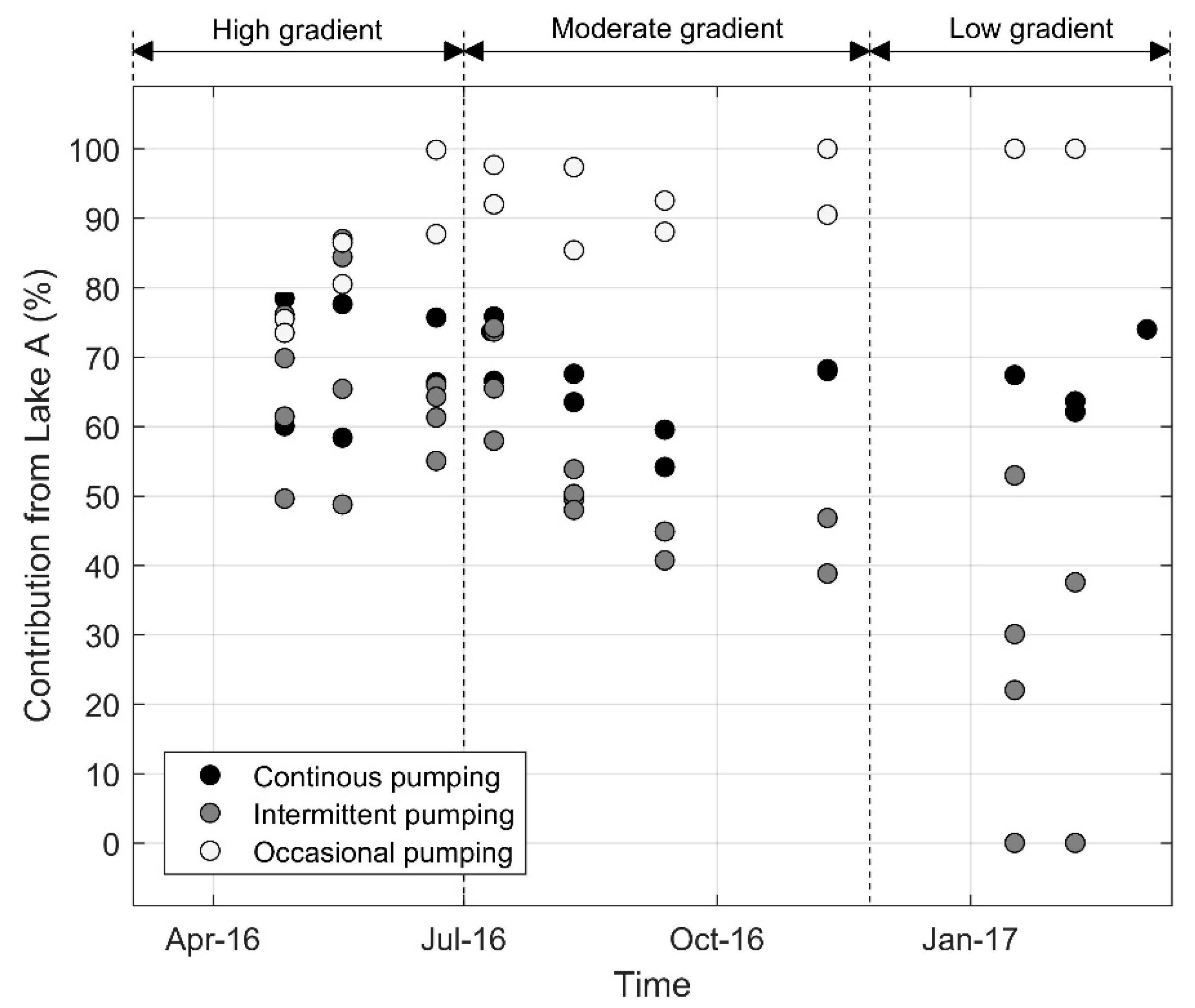
• All the pumping wells typically receive >50% of water from Lake A, but the competition between anthropic (i.e., pumping regime) and meteorological forcings (i.e., relative water level of both lakes) leads to a large variability of the mixing ratios (i.e., from 0% to 100% of water originating from Lake A);
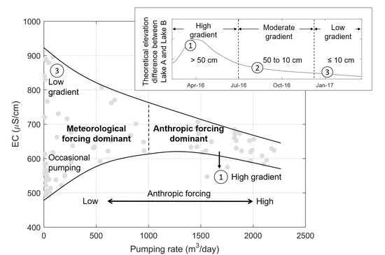
• When the meteorological forcing is high, the pumping regime has little influence over the origin of water and the mixing ratios are similar at all the pumping wells. When the meteorological forcing is low, the pumping regime is a decisive factor on the fraction of the contributing sources to the pumping wells;
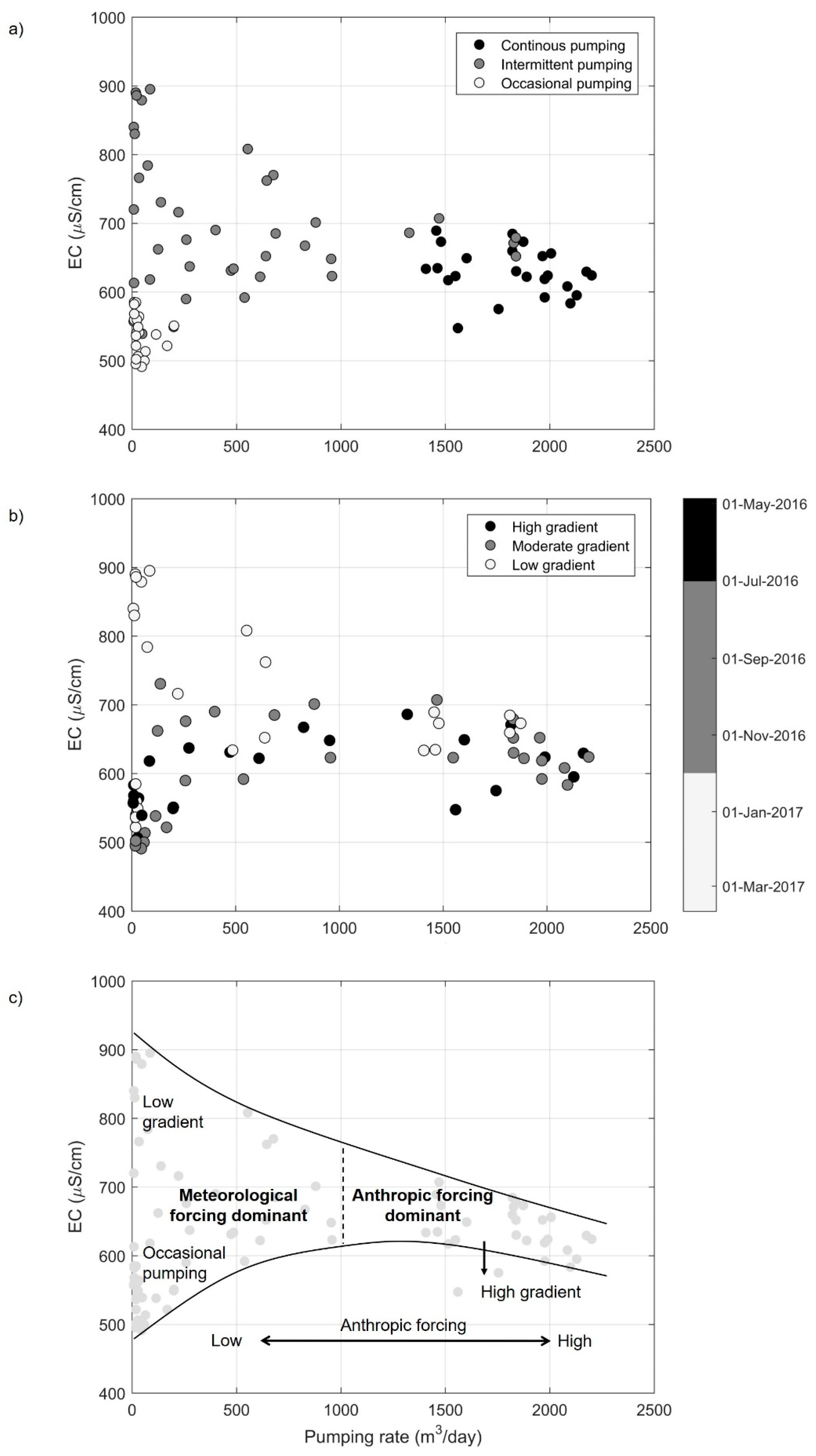
• When a pumping rate of >1000 m³/day is applied continuously, the mixing ratios are less variable due to direct anthropic forcing. When wells are operated only intermittently or occasionally and at a rate of <1000 m³/day, indirect anthropic and/or meteorological forcings govern the mixing ratio between Lake A and Lake B waters;
• A sensitivity analysis revealed that the relative estimation of the mixing ratios was acceptable and that measurement errors were not likely to influence our calculations. It also helped to quantify the importance of considering the temporal variability of the lakes’ end-members to obtain reliable results when estimating mixing ratios;
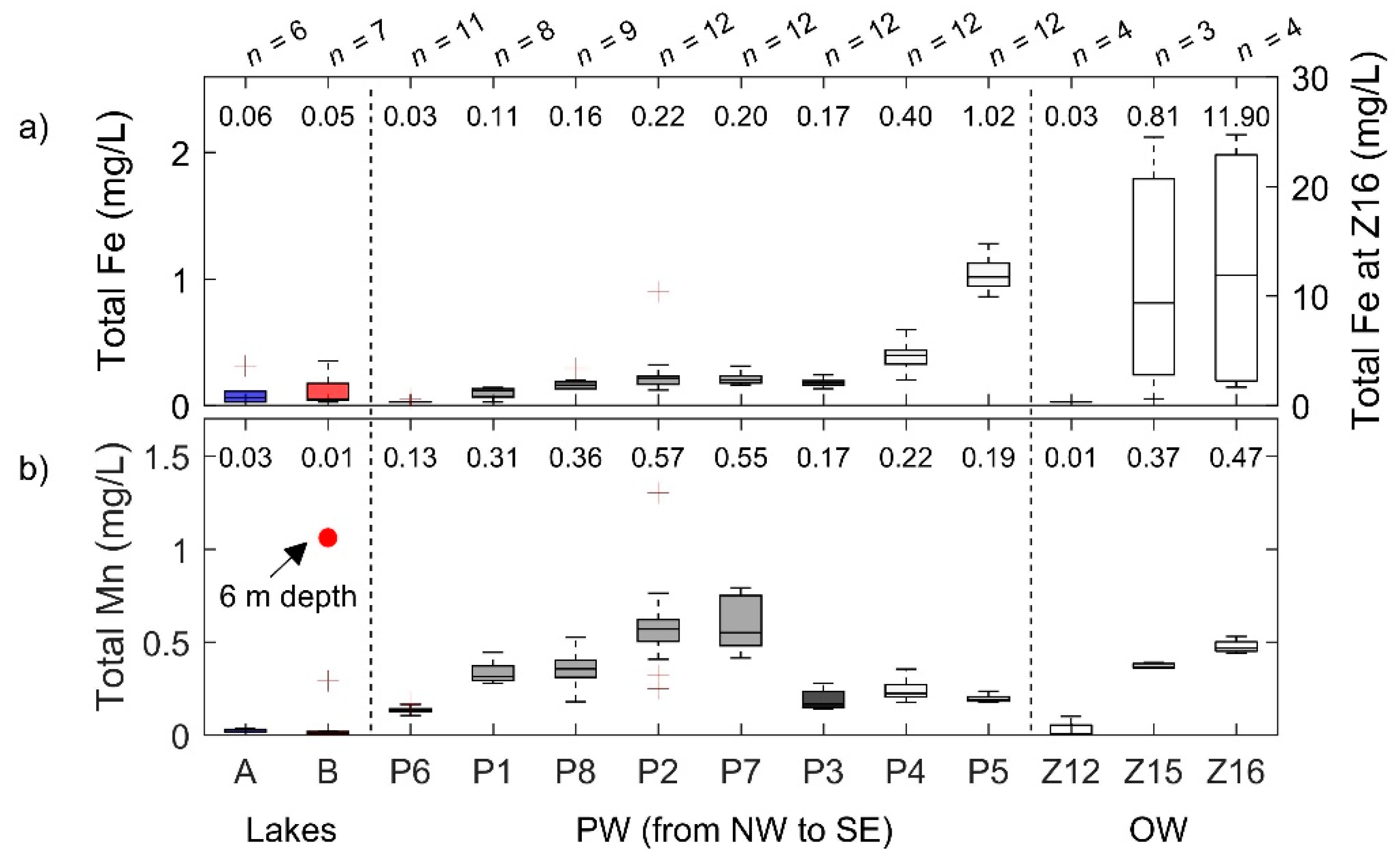
• The pumping regime influences total metals (i.e., Fe and Mn) concentrations in the raw abstracted waters. High Fe concentrations originate from particulate iron mobilization and resuspension when effective velocities of water entering the screens of the pumping wells are high, whereas high Mn concentrations are associated with an increase in the contribution from Lake B.

This study highlights how understanding the competition between anthropic and meteorological forcings can help to recommend guidelines for rapid decision-making regarding the quality of the pumped water. For instance, by identifying contexts for which the anthropic forcing is dominant, one can control the origin of the bank filtrate. Moreover, predicting periods under which the meteorological forcing is governing the flow patterns can help to adjust post-BF treatment in order to secure high quality of the distributed drinking water.

References

1. Haas, R.; Opitz, R.; Grischek, T.; Otter, P. The AquaNES project: Coupling riverbank filtration and ultrafiltration in drinking water treatment. Water 2018, 11, 18. [Google Scholar] [CrossRef]
2. Ross, A.; Hasnain, S. Factors affecting the cost of managed aquifer recharge (MAR) schemes. Sustain. Water Resour. Manag. 2018, 4, 179–190. [Google Scholar] [CrossRef]
3. Gillefalk, M.; Massmann, G.; Nutzmann, G.; Hilt, S. Potential impacts of induced bank filtration on surface water quality: A conceptual framework for future research. Water 2018, 10, 1240. [Google Scholar] [CrossRef]
4. Hiscock, K.M.; Grischek, T. Attenuation of groundwater pollution by bank filtration. J. Hydrol. 2002, 266, 139–144. [Google Scholar] [CrossRef]
5. Gunkel, G.; Hoffmann, A. Bank filtration of rivers and lakes to improve the raw water quality for drinking water supply. In Water Purification; Gertsen, N., Sonderby, L., Eds.; Nova Science Publishers, Inc.: Hauppauge, NY, USA, 2009; pp. 137–169. [Google Scholar]
6. Ronghang, M.; Gupta, A.; Mehrotra, I.; Kumar, P.; Patwal, P.; Kumar, S.; Grischek, T.; Sandhu, C. Riverbank filtration: A case study of four sites in the hilly regions of Uttarakhand, India. Sustain. Water Resour. Manag. 2019, 5, 831–845. [Google Scholar] [CrossRef]
7. Dash, R.R.; Prakash, E.V.P.B.; Kumar, P.; Mehrotra, I.; Sandhu, C.; Grischek, T. River bank filtration in Haridwar, India: Removal of turbidity, organics and bacteria. Hydrogeol. J. 2010, 18, 973–983. [Google Scholar] [CrossRef]
8. Sahu, R.L.; Dash, R.R.; Pradhan, P.K.; Das, P. Effect of hydrogeological factors on removal of turbidity during river bank filtration: Laboratory and field studies. Groundw. Sustain. Dev. 2019, 9, 100229. [Google Scholar] [CrossRef]
9. Harvey, R.W.; Metge, D.W.; LeBlanc, D.R.; Underwood, J.; Aiken, G.R.; Butler, K.; McCobb, T.D.; Jasperse, J. Importance of the colmation layer in the transport and removal of Cyanobacteria, viruses, and dissolved organic carbon during natural lake-bank filtration. J. Environ. Qual. 2015, 44, 1413–1423. [Google Scholar] [CrossRef]
10. Romero, L.G.; Mondardo, R.I.; Sens, M.L.; Grischek, T. Removal of Cyanobacteria and cyanotoxins during lake bank filtration at Lagoa do Peri, Brazil. Clean Technol. Environ. Policy 2014, 16, 1133–1143. [Google Scholar] [CrossRef]
11. Otter, P.; Malakar, P.; Sandhu, C.; Grischek, T.; Sharma, S.K.; Kimothi, P.C.; Nuske, G.; Wagner, M.; Goldmaier, A.; Benz, F. Combination of river bank filtration and solar-driven electro-chlorination assuring safe drinking water supply for river bound communities in India. Water 2019, 11, 122. [Google Scholar] [CrossRef]
12. Massmann, G.; Greskowiak, J.; Dunnbier, U.; Zuehlke, S.; Knappe, A.; Pekdeger, A. The impact of variable temperatures on the redox conditions and the behaviour of pharmaceutical residues during artificial recharge. J. Hydrol. 2006, 328, 141–156. [Google Scholar] [CrossRef]
13. Hamann, E.; Stuyfzand, P.J.; Greskowiak, J.; Timmer, H.; Massmann, G. The fate of organic micropollutants during long-term/long-distance river bank filtration. Sci. Total Environ. 2016, 545–546, 629–640. [Google Scholar] [CrossRef] [PubMed]
14. Grunheid, S.; Amy, G.; Jekel, M. Removal of bulk dissolved organic carbon (DOC) and trace organic compounds by bank filtration and artificial recharge. Water Res. 2005, 39, 3219–3228. [Google Scholar] [CrossRef] [PubMed]
15. Nagy-Kovacs, Z.; Laszlo, B.; Fleit, E.; Czihat-Martonne, K.; Till, G.; Bornick, H.; Adomat, Y.; Grischek, T. Behavior of organic micropollutants during river bank filtration in Budapest, Hungary. Water 2018, 10, 1861. [Google Scholar] [CrossRef]
16. Dragon, K.; Gorski, J.; Kruc, R.; Drozdzynski, D.; Grischek, T. Removal of natural organic matter and organic micropollutants during riverbank filtration in Krajkowo, Poland. Water 2018, 10, 1457. [Google Scholar] [CrossRef]
17. Greskowiak, J.; Prommer, H.; Massmann, G.; Nutzmann, G. Modeling seasonal redox dynamics and the corresponding fate of the pharmaceutical residue phenazone during artificial recharge of groundwater. Environ. Sci. Technol. 2006, 40, 6615–6621. [Google Scholar] [CrossRef]
18. Burke, V.; Greskowiak, J.; Asmuss, T.; Bremermann, R.; Taute, T.; Massmann, G. Temperature dependent redox zonation and attenuation of wastewater-derived organic micropollutants in the hyporheic zone. Sci. Total Environ. 2014, 482–483, 53–61. [Google Scholar] [CrossRef]
19. Munz, M.; Oswald, S.E.; Schafferling, R.; Lensing, H.J. Temperature-dependent redox zonation, nitrate removal and attenuation of organic micropollutants during bank filtration. Water Res. 2019, 162, 225–235. [Google Scholar] [CrossRef]
20. Groeschke, M.; Frommen, T.; Winkler, A.; Schneider, M. Sewage-borne ammonium at a river bank filtration site in Central Delhi, India: Simplified flow and reactive transport modeling to support decision-making about water management strategies. Geosciences 2017, 7, 48. [Google Scholar] [CrossRef]
21. Ahmed, A.K.A.; Marhaba, T.F. Review on river bank filtration as an in situ water treatment process. Clean Technol. Environ. Policy 2017, 19, 349–359. [Google Scholar] [CrossRef]
22. Jiang, Y.; Zhang, J.J.; Zhu, Y.G.; Du, Q.Q.; Teng, Y.G.; Zhai, Y.Z. Design and optimization of a fully-penetrating riverbank filtration well scheme at a fully-penetrating river based on analytical methods. Water 2019, 11, 418. [Google Scholar] [CrossRef]
23. Dillon, P.; Stuyfzand, P.; Grischek, T.; Lluria, M.; Pyne, R.D.G.; Jain, R.C.; Bear, J.; Schwarz, J.; Wang, W.; Fernandez, E.; et al. Sixty years of global progress in managed aquifer recharge. Hydrogeol. J. 2019, 27, 1–30. [Google Scholar] [CrossRef]
24. Kvitsand, H.M.L.; Myrmel, M.; Fiksdal, L.; Østerhus, S.W. Evaluation of bank filtration as a pretreatment method for the provision of hygienically safe drinking water in Norway: Results from monitoring at two full-scale sites. Hydrogeol. J. 2017, 25, 1257–1269. [Google Scholar] [CrossRef]
25. Derx, J.; Blaschke, A.P.; Farnleitner, A.H.; Pang, L.; Blöschl, G.; Schijven, J.F. Effects of fluctuations in river water level on virus removal by bank filtration and aquifer passage—A scenario analysis. J. Contam. Hydrol. 2013, 147, 34–44. [Google Scholar] [CrossRef] [PubMed]
26. Shamrukh, M.; Abdel-Wahab, A. Riverbank filtration for sustainable water supply: Application to a large-scale facility on the Nile River. Clean Technol. Environ. Policy 2008, 10, 351–358. [Google Scholar] [CrossRef]
27. Zhu, Y.G.; Zhai, Y.Z.; Du, Q.Q.; Teng, Y.G.; Wang, J.S.; Yang, G. The impact of well drawdowns on the mixing process of river water and groundwater and water quality in a riverside well field, Northeast China. Hydrol. Process. 2019, 33, 945–961. [Google Scholar] [CrossRef]
28. Dillon, P.J.; Miller, M.; Fallowfield, H.; Hutson, J. The potential of riverbank filtration for drinking water supplies in relation to microsystin removal in brackish aquifers. J. Hydrol. 2002, 266, 209–221. [Google Scholar] [CrossRef]
29. Gupta, A.; Singh, H.; Ahmed, F.; Mehrotra, I.; Kumar, P.; Kumar, S.; Grischek, T.; Sandhu, C. Lake bank filtration in landslide debris: Irregular hydrology with effective filtration. Sustain. Water Resour. Manag. 2015, 1, 15–26. [Google Scholar] [CrossRef]
30. Hu, B.; Teng, Y.G.; Zhai, Y.Z.; Zuo, R.; Li, J.; Chen, H.Y. Riverbank filtration in China: A review and perspective. J. Hydrol. 2016, 541, 914–927. [Google Scholar] [CrossRef]
31. AGEOS. Alimentation en eau Potable: Demande D’autorisation en Vertu de l’Article 31 du Règlement sur le Captage des Eaux Souterraines: Rapport D’expertise Hydrogéologique 2010-723; AGEOS: Brossard, QC, Canada, 2010; Volumes 1–2. [Google Scholar]
32. Pazouki, P.; Prevost, M.; McQuaid, N.; Barbeau, B.; de Boutray, M.L.; Zamyadi, A.; Dorner, S. Breakthrough of cyanobacteria in bank filtration. Water Res. 2016, 102, 170–179. [Google Scholar] [CrossRef]
33. Grischek, T.; Bartak, R. Riverbed clogging and sustainability of riverbank filtration. Water 2016, 8, 604. [Google Scholar] [CrossRef] [Green Version]
34. Pholkern, K.; Srisuk, K.; Grischek, T.; Soares, M.; Schafer, S.; Archwichai, L.; Saraphirom, P.; Pavelic, P.; Wirojanagud, W. Riverbed clogging experiments at potential river bank filtration sites along the Ping River, Chiang Mai, Thailand. Environ. Earth Sci. 2015, 73, 7699–7709. [Google Scholar] [CrossRef]
35. AGEOS. Alimentation en eau Potable: Suivi des Fluctuations Piézométriques de la Nappe et des Niveaux des Lacs: Période du 27 Avril 2012 au 17 Décembre 2015: Rapport Annuel 2015; 29 février 2016; AGEOS: Brossard, QC, Canada, 2016; p. 42. [Google Scholar]
36. Gran, G. Determination of the equivalence point in potentiometric titrations. Part II. Analyst 1952, 77, 661–671. [Google Scholar] [CrossRef]
37. Sprenger, C. Hydraulic Characterisation of Managed Aquifer Recharge Sites by Tracer Techniques; Demeau: Berlin, Germany, 2016; p. 15. [Google Scholar]
38. Baudron, P.; Barbecot, F.; Gillon, M.; Aróstegui, J.L.G.; Travi, Y.; Leduc, C.; Castillo, F.G.; Martinez-Vicente, D. Assessing groundwater residence time in a highly anthropized unconfined aquifer using bomb peak 14C and reconstructed irrigation water 3H. Radiocarbon 2013, 53, 933–1006. [Google Scholar] [CrossRef] [Green Version]
39. Baudron, P.; Sprenger, C.; Lorenzen, G.; Ronghang, M. Hydrogeochemical and isotopic insights into mineralization processes and groundwater recharge from an intermittent monsoon channel to an overexploited aquifer in eastern Haryana (India). Environ. Earth Sci. 2016, 75, 434. [Google Scholar] [CrossRef]
40. Boving, T.B.; Choudri, B.S.; Cady, P.; Cording, A.; Patil, K.; Reddy, V. Hydraulic and hydrogeochemical characteristics of a riverbank filtration site in rural India. Water Environ. Res. 2014, 86, 636–648. [Google Scholar] [CrossRef]
41. Buzek, F.; Kadlecova, R.; Jackova, I.; Lnenickova, Z. Nitrate transport in the unsaturated zone: A case study of the riverbank filtration system Karany, Czech Republic. Hydrol. Process. 2012, 26, 640–651. [Google Scholar] [CrossRef]
42. Glorian, H.; Bornick, H.; Sandhu, C.; Grischek, T. Water quality monitoring in Northern India for an evaluation of the efficiency of bank filtration sites. Water 2018, 10, 1804. [Google Scholar] [CrossRef] [Green Version]
43. Lorenzen, G.; Sprenger, C.; Baudron, P.; Gupta, D.; Pekdeger, A. Origin and dynamics of groundwater salinity in the alluvial plains of western Delhi and adjacent territories of Haryana State, India. Hydrol. Process. 2012, 26, 2333–2345. [Google Scholar] [CrossRef]
44. Wett, B.; Jarosch, H.; Ingerle, K. Flood induced infiltration affecting a bank filtrate well at the River Enns, Austria. J. Hydrol. 2002, 266, 222–234. [Google Scholar] [CrossRef]
45. Government of Canada. Guidelines for Canadian Drinking Water Quality: Guideline Technical Document–Iron. Available online: https://www.canada.ca/en/health-canada/services/publications/healthy-living/guidelines-canadian-drinking-water-quality-guideline-technical-document-iron.html (accessed on 9 August 2019).
46. Government of Canada. Guidelines for Canadian Drinking Water Quality: Guideline Technical Document–Manganese. Available online: https://www.canada.ca/en/health-canada/services/publications/healthy-living/guidelines-canadian-drinking-water-quality-guideline-technical-document-manganese.html (accessed on 9 August 2019).
47. Arnoux, M.; Gibert-Brunet, E.; Barbecot, F.; Guillon, S.; Gibson, J.; Noret, A. Interactions between groundwater and seasonally ice-covered lakes: Using water stable isotopes and radon-222 multilayer mass balance models. Hydrol. Process. 2017, 31, 2566–2581. [Google Scholar] [CrossRef]
48. Des Tombe, B.F.; Bakker, M.; Schaars, F.; van der Made, K.J. Estimating travel time in bank filtration systems from a numerical model based on DTS measurements. Ground Water 2018, 56, 288–299. [Google Scholar] [CrossRef] [PubMed] [Green Version]
49. Glass, J.; Li, T.; Sprenger, C.; Stefan, C. Investigation of viscosity effects caused by seasonal temperature fluctuations during MAR. In Proceedings of the International Symposium on Managed Aquifer, Madrid, Spain, 20–24 May 2019. [Google Scholar]
50. Liu, S.D.; Zhou, Y.X.; Kamps, P.; Smits, F.; Olsthoorn, T. Effect of temperature variations on the travel time of infiltrating water in the Amsterdam Water Supply Dunes (The Netherlands). Hydrogeol. J. 2019, 27, 2199–2209. [Google Scholar] [CrossRef]
51. Henzler, A.F.; Greskowiak, J.; Massmann, G. Seasonality of temperatures and redox zonations during bank filtration—A modeling approach. J. Hydrol. 2016, 535, 282–292. [Google Scholar] [CrossRef]
52. Grischek, T.; Paufler, S. Prediction of iron release during riverbank filtration. Water 2017, 9, 317. [Google Scholar] [CrossRef] [Green Version]
Figure 1. Study site location maps (ac) and schematic lithological cut along pumping wells (d) (adapted with permission from Ageos, 2010 [31]).
Water 11 02510 g001
Figure 2. Schematic representation of the flow patterns and directions at the study site when (a) elevation of Lake B > elevation of Lake A, (b) elevation of Lake A > elevation of Lake B, and (c) the pumping wells are in operation. Black, blue, and red arrows refer to regional groundwater and water originating from Lake A and Lake B, respectively. Theoretical elevation difference between Lake A and Lake B in (d). Numbers 1 to 3 correspond to different hydraulic conditions, namely high, moderate, and low hydraulic gradients between Lake A and Lake B.
Water 11 02510 g002
Figure 3. Pumping rates for wells (a) P1, (b) P3, (c) P5, and (d) P6 during a typical one-week period (from 16 January 2017 to 23 January 2016). Monitoring and water sampling were conducted on 17 January 2017 at all the pumping wells.
Water 11 02510 g003
Figure 4. Monthly mean total pumping rate from March 2016 to March 2017. Above each bar are the proportions of the total pumped volume supplied by the continuously (in black) and intermittently (in grey) pumping wells. The occasionally pumping wells supply only <1–2% of the total pumped volume.
Water 11 02510 g004
Figure 5. Boxplots of (a) temperature, (b) electrical conductivity (EC), (c) pH, and (d) redox potential (Eh) at the lakes, pumping wells (PW), and observation wells (OW). Blue and red boxes are associated with Lake A (<1 m depth) and Lake B (<1 m depth), whereas dark, medium, and light grey boxes correspond to continuously, intermittently, and occasionally pumping wells, respectively. Numeric values above each box correspond to the median.
Water 11 02510 g005
Figure 6. Boxplots of (a) total Fe, and (b) total Mn concentrations at the lakes, pumping wells, and piezometers. Blue and red boxes are associated with Lake A (<1 m depth) and Lake B (<1 m depth), whereas dark, medium, and light grey boxes correspond to continuously, intermittently, and occasionally pumping wells, respectively. Numeric values above each box correspond to the median. Red circle represents the maximal observed total Mn in Lake B (at 6 m depth).
Water 11 02510 g006
Figure 7. Comparison of the geochemical facies of Lake A, Lake B, pumping wells, and the regional groundwater (GW). The solid black line represents the mixing line between Lake A and Lake B mean values.
Water 11 02510 g007
Figure 8. Time series of electrical conductivity (EC) at (a) Lake A (<1 m depth), and (b) Lake B (<1 m depth) and Z12. The grey shaded area represents the timing for hydraulic connection between Lake A and Lake C. Error bars (±20 µS/cm) represent the maximal expected measurement error on EC. The yellow dashed line corresponds to the mean EC value at Z12.
Water 11 02510 g008
Figure 9. Electrical conductivity (EC) measurements against depth at Lake A and Lake B in winter and summer. Solid lines represent depth-average value at the lakes, while the yellow dashed line is associated with mean EC values at observation well Z12. Blue and red shaded areas illustrate the variability in EC at the surface (<1 m depth) of Lake A and Lake B, respectively.
Water 11 02510 g009
Figure 10. Estimated contribution from Lake A to the pumping wells according to the reference scenario. Lake A end-member is defined as a time-varying electrical conductivity (EC) signal, which was derived from the observed EC values at <1 m depth. Lake B end-member is a fixed EC value which corresponds to the mean of the wintertime and summertime depth-average value.
Water 11 02510 g010
Figure 11. Relationship between electrical conductivity (EC) and the one-month average pumping rate prior to the sampling date, according to (a) the pumping regime and (b) the hydraulic gradient between Lake A and Lake B. A schematic representation of the dominant forcing is illustrated in (c), where solid and dashed lines represent the range of observed values and the delimitation between regimes where meteorological and anthropic forcings are dominant, respectively.
Water 11 02510 g011
Figure 12. Relationship between (a) total Fe and (b) total Mn concentrations and the 1-month average pumping rate prior to the sampling date.
Water 11 02510 g012