Experimental and Numerical Study on Water Filling and Air Expelling Process in a Pipe with Multiple Air Valves under Water Slow Filling Condition

Abstract

This paper investigates the physical processes involved in the water filling and air expelling process of a pipe with multiple air valves under water slow filling condition, and develops a fully coupledwater–air two-phase stratified numerical model for simulating the process. In this model, the Saint-Venant equations and the Vertical Average Navier–Stokes equations (VANS) are respectively applied to describe the water and air in pipe, and the air valve model is introduced into the VANS equations of air as the source term. The finite-volume method and implicit dual time-stepping method (IDTS) with two-order accuracy are simultaneously used to solve this numerical model to realize the full coupling between water and air movement. Then, the model is validated by using the experimental data of the pressure evolution in pipe and the air velocity evolution of air valves, which respectively characterize the water filling and air expelling process. The results show that the model performs well in capturing the physical processes, and a reasonable agreement is obtained between numerical and experimental results. This agreement demonstrates that the proposed model in this paper offers a practical method for simulating water filling and air expelling process in a pipe with multiple air valves under water slow filling condition.

1. Introduction

In the water filling stage of a pipe, the initial air inside the pipe will start a deformation under the influence of water filling the pipe. If the air is not expelled appropriately, it will accumulate in the pipe and create overpressure affecting the pipe safety [1]. Installing air valves to expel air from the pipe is an effective way to control overpressure. However, the process of water filling and air expelling in the pipe highly depends on the air valve layout including the location and quantity [1,2].

Numerical models are important tools for simulating the evolution of water and air in pipe system. Affected by the change of water-flow rate and pipe elevation, the water flow is unsteady with free surface flows, pressurized flows and free-surface-pressurized flows occurred concurrently or separately. Many Preissmann slot methods have been established for simulating these unsteady water flows, which are also applicable to simulate unsteady water flow during pipe filling [3,4,5,6,7]. However, for simulating the air evolution and air expelling inside the pipe, the water–air two-phase model is needed. Determining the water–air two-phase flow pattern is the basis to establish a suitable two-phase model. Taitel et al. summarized six types flow patterns of water and air in horizontal pipe or near-horizontal pipe [8], which includes stratified smooth flow, stratified wavy flow, bubble flow, slug flow, plug flow and annular flow. According to different flow patterns, the models used to simulate the evolution of water and air in pipe can be divided into drift-flux model and two-phase model [9]. The drift-flux model regards the air and water as a mixture and writes a single momentum conservation equation for the mixture, and the two-phase velocities are expressed explicitly by the algebraic formula through the mixture velocity [10]. The drift-flux model is originally proposed for bubble flow and extended later to cover the entire range of flow patterns that may occur in water–air two-phase flow in inclined pipe [11,12,13,14]. However, due to the inherent limitation of the drift-flux model, this model is not suitable for the simulation of the flow patterns with distinct stratification such as stratified smooth flow and stratified wavy flow in horizontal or near-horizontal pipe.

The two-phase model, including one-dimensional models and three-dimensional models, are suitable for flow patterns with obvious stratification [15,16,17,18]. Because of the two-phase flow in engineering applications in pipe system is computationally unapproachable in a three-dimensional context [19], one-dimensional models are developed widely. In the one-dimensional two-phase model, each phase is considered separately, thus the model consist of two separate sets of balance equations and the interactions between the phases are modeled through additional terms in these equations. A fully developed water–air two-phase flow model includes mass, momentum and energy equations for water and air in pipe, respectively. However, many two-phase flow models reduce the number of variables or governing equations based on the hypothesis for different specific problems, which not only simplifies the model but also guarantees the applicability of the model. At present, the main hypothesis is that water is an incompressible fluid, and its evolution in pipe is isothermal with the steady friction factor, and for the air evolution, it is assumed as an adiabatic process or an isothermal process [20,21,22,23].

Air valves in the delivery pipe allow air inside pipe to expel when the pipe becomes overpressurized. By far, for simulating the air valve behavior, it is common to make an analogy between the air flow through an air valve and isentropic flow in nozzles [24].Wang et al. modeled the air expelling by making a pipe with only one air valve under rapid water filling and making a judgment about the relative position of the flow front and the air valve [25]; such an approach is too complex to be applied for pipes with multiple air valves. Miquel et al. established a model to simulate the air expelling of a pipe with an air valve only at the end of the pipe under rapid water filling, and air valve is only considered as the downstream boundary in the model [1]. Coronado-Hernández et al. developed a mathematical model for a single pipe with an air valve and the model provides good accuracy under rapid water filling [26].

All the models mentioned above are developed by assuming a vertical interface between the air and water and are applied for pipe under rapid water filling condition, which are no longer applicable to predict the behavior of air expelling of a pipe with multiple air valves under water slow filling condition with sufficient accuracy. Therefore, it is necessary to study the characteristics of water filling and air expelling process of a pipe with multiple air valves under water slow filling condition and develop a fully coupled numerical model for simulating the process. This is the main purpose of this study.

In this paper, a laboratory experimental system is established for observing the change of water–air two phases flow pattern in pipe during water slow filling, then a water–air two-phase stratified model is developed. The Saint-Venant equations based on the concept of the Preissmann slot and the Vertical Average Navier–Stokes equations (VANS) are applied to describe the evolution of water flow and air in pipe, respectively. Meanwhile, an improved air valve model based on the method proposed by Wylie [24] is introduced into the VANS equations of air as the source term, combining the finite-volume method and implicit dual time-stepping method (IDTS) with two-order accuracy for solving this numerical model. A detailed discussion about water–air interface assumption and some explanations for the numerical model are given further, based on the test results and published relevant literatures. Finally, the experimental results are used for validation of this proposed numerical model.

2. Materials and Methods

2.1. Experimental Setup

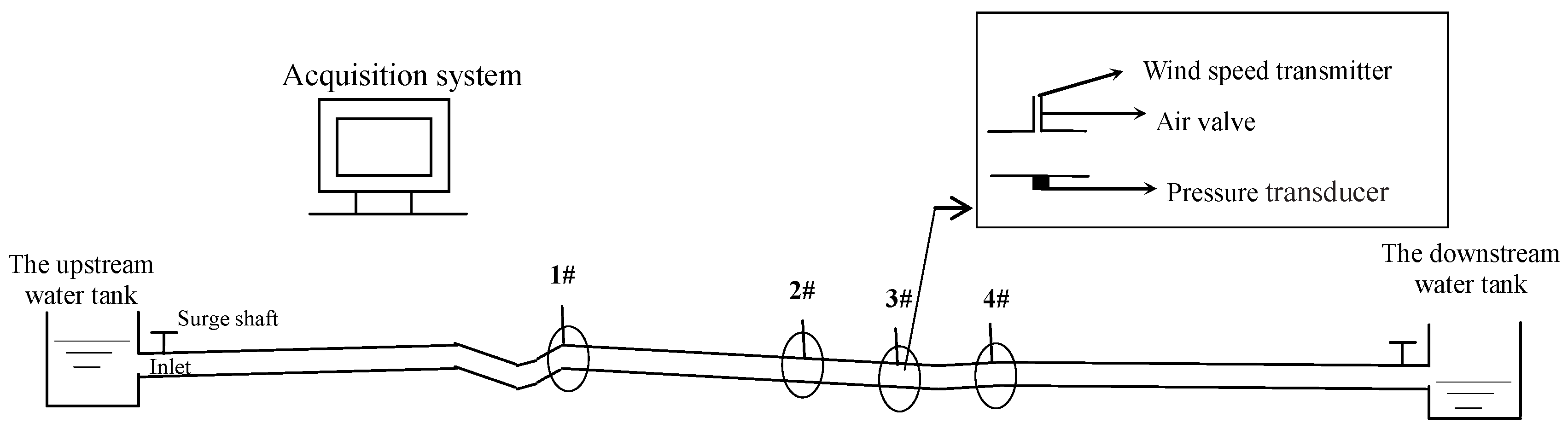
The laboratory experimental system consists of an upstream water supply tank, a surge shaft, a test pipe, four air valves, a downstream water tank, and measurement facilities (see Figure 1). The test pipe is made of plexiglas material with total length, inner diameter and Manning roughness coefficient of 300 m, 240 mm and 0.0088, respectively, which is well fixed onto the ground through a number of iron stands along the pipe.

There are four common air valves with inner diameter of 24 mm installed on the measuring point and air inside the pipe can be expelled out by the air valves without limitation of air valve’s construction. There are four pressure transducers installed at four measuring points. The pressure transducers are installed at the bottom of the pipe to record the pressure changes inside the pipe. Meanwhile, four wind speed transmitters are installed at the top of the air valves to record the air velocity though the air valves. Both the measured data are collected by the acquisition system. The details of this system is shown in

Table 1. The parameters of the testing pipeline.

Air Valve	Distance to the Inlet (m)	Relative Elevation (mm)	Pipe Length (m)	Slope (‰)
	0	156	60.578	−3.527
	60.578	370
			7.014	+49.985
	67.592	24
			4.200	0
	71.792	24
			1.990	−50.197
1#	73.782	113
			60.640	+1.000
2#	134.422	53
			22.210
3#	156.632	31
			29.880
	186.512	0
			20.684	−4.877
4#	207.196	92
			93.146	−0.202
	300.342	116

.

For testing, water is supplied from the upstream water tank to the pipe with a steady and constant pressure head and discharged into the downstream water tank (with lower water level than downstream pipe). The water flow rate in the pipe is controlled and adjusted at expected level of 14.47 m³/h by the surge shaft at the end of upstream pipe. During the test, high-speed cameras are used to take high-resolution pictures of the flow patterns in the pipe.

2.2. Numerical Model

To develop the numerical model, it is assumed that the water is incompressible, whereas the air is compressible. The mass exchange, heat transfer and temperature change between water and air in pipe are neglected. Meanwhile, in order to calculate the unsteady mixed water flow in pipe, the free surface flows, pressurized flows and free-surface-pressurized flows are uniformly expressed by the conservative form of Saint-Venant equations with the concept of the Preissmann slot [27]. Thus, the water and air are described by Saint-Venant equations [Equations (1a) and (1b)] and VRNS equations [Equations (2a) and (2b)], respectively.

$$\frac{\partial A_w}{\partial t}+\frac{\partial Q_w}{\partial x} = 0$$

(1a)

$$\frac{\partial Q_w}{\partial t}+\frac{\partial \left(Q_w{u}_w\right)}{\partial x} = -\mathrm{g}{A}_w\frac{\partial \zeta }{\partial x}-\mathrm{g}\frac{n^2{Q}_w\left|u_w\right|}{R^{4/3}}$$

(1b)

$$\frac{\partial {\overline{m}}_a}{\partial t}+\frac{\partial m_a}{\partial x} = -\Gamma \left(x_L\right)\dot{m}$$

(2a)

$$\frac{\partial \left(m_a\right)}{\partial t}+\frac{\partial \left(m_a{u}_a\right)}{\partial x} = -A_w\frac{\partial P_1}{\partial x}-A_a\frac{\partial P_2}{\partial x}$$

(2b)

where $t$ is the temporal coordinate (s); $x$ is the spatial coordinate along pipe (m); $A_w$ is the cross-section area of flow (m²); $u_w$ is the uniform velocity along the pipe cross-section of flow (m/s); $Q_w$ is the discharge along the pipe cross-section of flow (m³/s), and $Q_w = A_w{u}_w$; ${\overline{m}}_a$ is the air mass flux along the pipe cross-section (Kg/m), and ${\overline{m}}_a = {\rho }_a{A}_a$, with ${\rho }_a$ as the density of air phase in pipe (kg/m³) and $A_a$ as the cross-sectional area of air (m²); $u_a$ is the average velocity along the pipe cross-section of air (m/s); $m_a$ is the air mass flow rate along the pipe cross-section (Kg/s), and $m_a = {\rho }_a{A}_a{u}_a = {\overline{m}}_a{u}_a$; $\zeta = z_b+h$ is the water piezometric head or water free-surface elevation, with $z_b$ as the pipe bottom elevation (m) and $h$ as the water level in pipe (m); $\mathrm{g}$ is the gravitational acceleration, 9.8 m/s²; $R$ is the hydraulic radius (m), $R$ has its own different expression for free surface flow and pressurized water flow in pipe due to the concept of the Preissmann slot, andis calculated by using the expressions in Liu’s paper [28]; $n$ is the Manning roughness coefficient (s/m^1/3); $\Gamma \left(x_L\right)\dot{m}$ is the air expelling mass flow rate per unit length (Kg/(s·m)), and $x_L$ represents the air valve position. $P_1$ is the pressure of the air in the pipe when the water enters the pipe (Pa); $P_2$ is the pressure of the air in the pipe because of its own compressibility (Pa).

For any cross-section of the pipe, $A_a$ and $A_w$ subject to the condition as follows:

$$A_a+A_w = A$$

(3)

where A is the cross-sectional area of pipe (m²).

The expression of $\Gamma \left(x_L\right)$ in Equation (2a) is as follows:

$$\Gamma \left(x_L\right) = \{\begin{array}{c}1, \mathrm{if} x = x_l\\ 0, \mathrm{if} x\ne x_l\end{array}$$

(4)

where $\Gamma \left(x_L\right) = 1$ representsan air valvehere, and $\Gamma \left(x_L\right) = 0$ representsnoair valve.

Based on the method proposed by Wylie [24], an improved form for calculating the source term $\dot{m}$ in Equation (2a) can be expressed in two cases as follows:

$$\dot{m} = \{\begin{array}{cc}\hfill \frac{C_d{A}_{v}P}{L}\sqrt{\frac{7}{R^{*}T}\left[{\left(\frac{P_{atm}}{P}\right)}^{1.4286}-{\left(\frac{P_{atm}}{P}\right)}^{1.7143}\right]}, & P_{atm}<P<1.894P_{atm}\hfill \\ \hfill \frac{C_d{A}_{v}P}{L}\frac{0.6847}{\sqrt{R^{*}T}}, & P>1.894P_{atm}\hfill \end{array}$$

(5)

where, $C_d$ is the air flow coefficient, $A_v$ is the air orificecross-sectional area (m²), $R^{*}$ is the universal air constant, 8.314 J/(mol·K); T is the absolute kelvin temperature of the air in pipe (K); $P_{atm}$ is the atmospheric pressure (Pa); $L$ is the pipe length (m); $P$ is the absolute pressure at inlet of air valve (Pa), and expressed as follows:

$$P = P_1+P_2$$

(6)

$P_1$ in Equations (2b) and (6) is the pressure of the air in the pipe when the water is filling the pipe, $P_1$ two wayscan be defined based on the hydrodynamic or hydrostatic scheme [29]. In this paper, we use the hydrostatic scheme and adopt the following expressions:

$$P_1 = {\rho }_w\mathrm{g}h$$

(7)

where, ${\rho }_w$ = water density, and its value is equal to 1000 kg/m³ due to treat water as incompressible.

$P_2$ in Equations (2b) and (6) is the pressure of the air in the pipe because of its compressibility. Both amount and volume of the air are changed when the air valves are installed, and the direct indicator of the air compressibility is the air density in the pipe. According to the ideal gas law, the expression of $P_2$ is as follows:

$$P_2 = {\rho }_a{R}^{**}T$$

(8)

where, $R^{**}$ is also a universal air constant, 286.7.

In more detail, we also give the relationship between mass flow rate $\dot{m}$ and air velocity $v_a$ as follows:

$$v_a=\dot{m}/{\rho }_v{A}_v$$

(9)

where ${\rho }_v$ is the density of the air in air valves; in this paper, ${\rho }_v = {\rho }_{atm}$, and ${\rho }_{atm}$ is the air density under atmospheric pressure. According to the Equation (9), we can obtain the calculated air velocity $u_v$ by the numerical model.

2.3. Numerical Solutions

In numerical solutions, the vector form of Equations (1) and (2) are commonly used:

$$\frac{\partial U}{\partial t}+\frac{\partial F}{\partial x} = S_P+S_f+S_{out}$$

(10)

where U is dependent variable vector; $F=uU$ is the advection flux, and $u$ respectively represents $u_w$ and $u_a$ for water and air; $S_P$, $S_f$ and $S_{out}$ are source terms pertaining to the pressure gradient term, the friction term, and the air-expelling term, respectively. These terms are written as follows:

$$\begin{array}{c}\mathbf{U}=\left[\begin{array}{c}{A}_w\\ Q_w\\ {\overline{m}}_a\\ m_a\end{array}\right],\mathbf{F}=u\mathbf{U}=\left[\begin{array}{c}{A}_w{u}_w\\ Q_w{u}_w\\ {\overline{m}}_a{u}_a\\ m_a{u}_a\end{array}\right],{\mathbf{S}}_P=\left[\begin{array}{c}0\\ -\mathrm{g}Aw\frac{\partial \zeta }{\partial x}\\ -A_w\frac{\partial P_1}{\partial x}-A_a\frac{\partial P_2}{\partial x}\end{array}\right],\\ {\mathbf{S}}_f=\left[\begin{array}{c}0\\ -\mathrm{g}\frac{n^2{Q}_w\left|u_w\right|}{R^{4/3}}\\ 0\\ 0\end{array}\right],{\mathbf{S}}_{out}=\left[\begin{array}{c}0\\ 0\\ -\Gamma (x_L)\dot{m}\\ 0\end{array}\right]\end{array}$$

(11)

2.3.1. Two-Order Reconstruction of the Flow Variable

The variables of water and air in dependent variable vector $U$ in two faces of the cell interface (i + 1/2) are reconstructed spatially as follows:

$$U_{i+1/2,L}=U_i+\frac{1}{2}\Delta U_i, U_{i+1/2,R}=U_i-\frac{1}{2}\Delta U_{i+1}$$

(12)

where subscript L and R represent the left and right condition of cell interface (i + 1/2), respectively. The values of $\Delta U_i$ and $\Delta U_{i+1}$ in Equation (12) are calculated using the minmod limiter [30].

2.3.2. Spatial Discretization

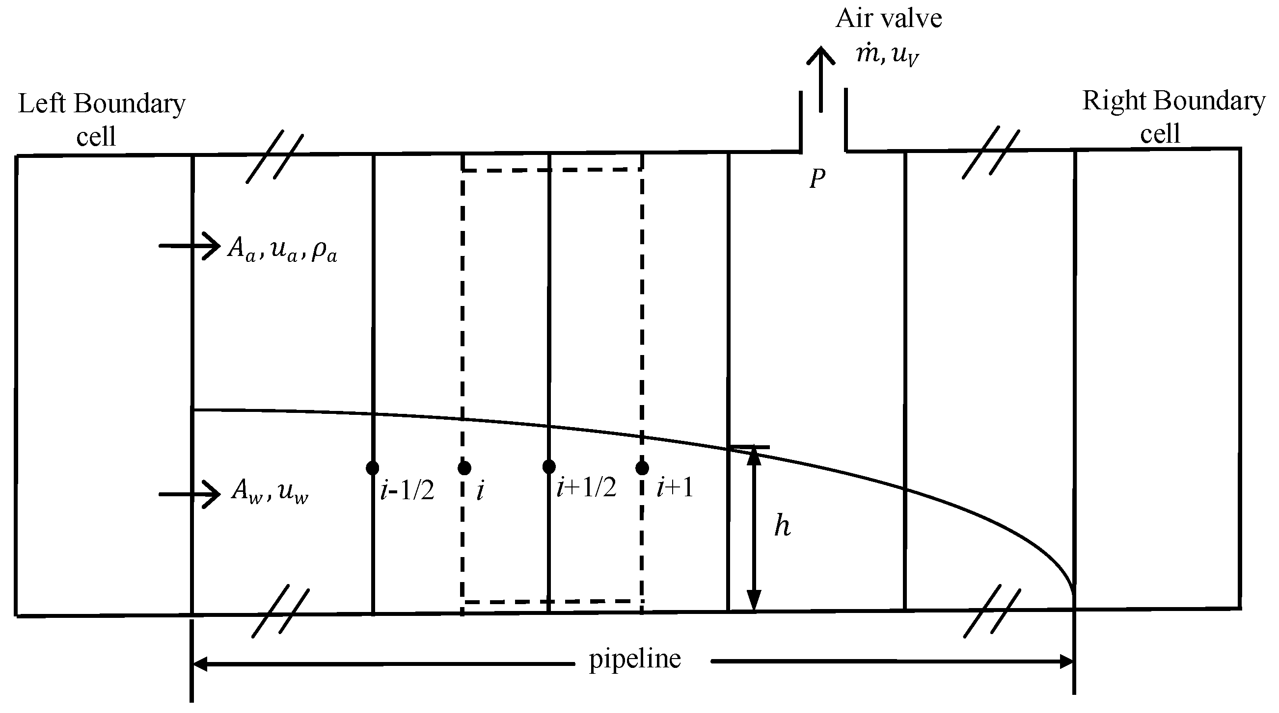
The integral of Equation (10) in any cell i (see Figure 2) is given as follows:

$${{\displaystyle \int }}_{i-1/2}^{i+1/2}\frac{\partial U}{\partial t}dx+{{\displaystyle \int }}_{i-1/2}^{i+1/2}\frac{\partial \left(uU\right)}{\partial x}dx = {{\displaystyle \int }}_{i-1/2}^{i+1/2}{S}_{P}dx+{{\displaystyle \int }}_{i-1/2}^{i+1/2}{S}_{f}dx+{{\displaystyle \int }}_{i-1/2}^{i+1/2}{S}_{out}dx$$

(13)

where subscripts (i + 1/2) and (i − 1/2) represent the left and right interfaces of the spatial cell i, respectively.

According to the divergence theorem [30], the second term on the left side of Equation (13) is expressed as follows:

$${{\displaystyle \int }}_{i-1/2}^{i+1/2}\frac{\partial \left(uU\right)}{\partial x}dx = {\left(uU\right)}_{i+1/2}-{\left(uU\right)}_{i-1/2}$$

(14)

where ${\left(uU\right)}_{i+1/2}$,${\left(uU\right)}_{i-1/2}$ are the numerical fluxes at interfaces (i + 1/2) and (i − 1/2), respectively. ${\left(uU\right)}_{i+1/2}$ is defined as follows [31]:

$${\left(uU\right)}_{i+1/2} = \frac{1}{2}{\tilde{c}}_{i+1/2}{F}_{i+1/2}\left(U_{i+1/2,L}+U_{i+1/2,R}\right)-\frac{1}{2}{\tilde{c}}_{i+1/2}\left|F_{i+1/2}\right|\left(U_{i+1/2,R}+U_{i+1/2,L}\right)$$

(15)

where ${\tilde{c}}_{i+1/2}$ represents the gravitational wave velocity of free surface wateror the acoustic wave speed of pressurized water for pressurized water or the acoustic wave speed of air in pipe at interface (i + 1/2) (m/s). $F_{i+1/2} = u_{i+1/2}/{\tilde{c}}_{i+1/2}$ is the Froude number for water or the Mach number for air at interface (i + 1/2). The definitions of ${\tilde{c}}_{i+1/2}$ and $F_{i+1/2}$ in Equation (15) are expressed as follows:

$${\tilde{c}}_{i+1/2} = \frac{1}{2}\left({\tilde{c}}_{i+1/2,L}+{\tilde{c}}_{i+1/2,R}\right)F_{i+1/2} = {\lambda }_{i+1/2,L}+{\lambda }_{i+1/2,R}$$

(16)

where ${\lambda }_{i+1/2,L}$ and ${\lambda }_{i+1/2,R}$ are the splitting functions of the $F$ at cell interfaces (i + 1/2) and are expressed as follows:

$$\begin{gathered} {\lambda }_{i+1/2,L} = \{\begin{array}{c}\hfill \frac{1}{4}{\left(F_{i+1/2,L}+1\right)}^2, \left|F_{i+1/2,L}\right|\le 1\\ \frac{1}{2}\left(F_{i+1/2,L}+\left|F_{i+1/2,L}\right|\right), \left|F_{i+1/2,L}\right|>1\hfill \end{array} \\ {\lambda }_{\mathrm{i}+1/2,\mathrm{R}}=\{\begin{array}{c}\hfill -\frac{1}{4}{\left(F_{\mathrm{i}+1/2,\mathrm{R}}-1\right)}^2, \left|F_{\mathrm{i}+1/2,\mathrm{R}}\right|\le 1\\ \frac{1}{2}\left(F_{\mathrm{i}+1/2,\mathrm{R}}-\left|{\mathrm{F}}_{\mathrm{i}+1/2,\mathrm{R}}\right|\right), \left|F_{\mathrm{i}+1/2,\mathrm{R}}\right|>1\hfill \end{array} \end{gathered}$$

(17)

Based on Equation (15), $F_{i+1/2,L}$ and $F_{\mathrm{i}+1/2,\mathrm{R}}$ in Equations (17) are expressed as follows:

$$F_{i+1/2,L} = \frac{u_{i+1/2,L}}{{\tilde{c}}_{i+1/2,L}}, F_{i+1/2,R} = \frac{u_{i+1/2,R}}{{\tilde{c}}_{i+1/2,R}}$$

(18)

Equation (15) can also be rewritten as follows:

$$\begin{array}{cc}\hfill {\left(uU\right)}_{i+1/2} =& \frac{1}{2}{\tilde{c}}_{i+1/2}{F}_{i+1/2}\left(U_{i+1}+U_i+\frac{1}{2}\Delta U_i-\frac{1}{2}\Delta U_{i+1}\right)\hfill \\ & -\frac{1}{2}{\tilde{c}}_{i+1/2}\left|F_{i+1/2}\right|\left(U_{i+1}-U_i-\frac{1}{2}\Delta U_{i+1}-\frac{1}{2}\Delta U_i\right)\hfill \end{array}$$

(19)

${\left(uU\right)}_{i-1/2}$ is expressed similarly, consequently Equation (14) is given as follows:

$${\left(uU\right)}_{i+1/2}-{\left(uU\right)}_{i-1/2} = {\mathit{\alpha }}_i{U}_{i-1}+{\mathit{\beta }}_i{U}_i+{\mathit{\gamma }}_i{U}_{i+1}+{\mathit{\eta }}_i$$

(20)

$${\mathit{\alpha }}_i = \frac{1}{2}{\tilde{c}}_{i-1/2}\left(F_{i-1/2}-\left|F_{i-1/2}\right|\right)$$

(21a)

$${\mathit{\beta }}_i = \frac{1}{2}\left[{\tilde{c}}_{i+1/2}\left(F_{i+1/2}-\left|F_{i+1/2}\right|\right)-{\tilde{c}}_{i-1/2}\left(F_{i-1/2}-\left|F_{i-1/2}\right|\right)\right]$$

(21b)

$${\mathit{\gamma }}_i = \frac{1}{2}{\tilde{c}}_{i+1/2}\left(F_{i+1/2}-\left|F_{i+1/2}\right|\right)$$

(21c)

$$\begin{array}{cc}\hfill {\mathit{\eta }}_i =& -\frac{1}{4}{\tilde{c}}_{i+1/2}\left(\left|F_{i+1/2}\right|-F_{i+1/2}\right)\Delta U_{i+1}\hfill \\ & \hspace{1em}\hspace{1em}+\frac{1}{4}\left[{\tilde{c}}_{i+1/2}\left(F_{i+1/2}+\left|F_{i+1/2}\right|\right)+{\tilde{c}}_{i-1/2}\left(F_{i-1/2}-\left|F_{i-1/2}\right|\right)\right]\Delta U_i\hfill \\ & \hspace{1em}\hspace{1em}-\frac{1}{4}{\tilde{c}}_{i-1/2}\left(F_{i-1/2}+\left|F_{i-1/2}\right|\right)\Delta U_{i-1}\hfill \end{array}$$

(21d)

Equation (21d) includes four components, namely ${\eta }_{\mathrm{wmass},i}$, ${\eta }_{\mathrm{wmomentum},i}$, ${\eta }_{\mathrm{amass},i}$ and ${\eta }_{\mathrm{wmomentum},i}$ as follows:

$$\begin{array}{cc}\hfill {\eta }_{\mathrm{wmass},i}=& -\frac{1}{4}{\tilde{c}}_{i+1/2}\left(\left|F_{i+1/2}\right|-F_{i+1/2}\right)\Delta A_{w,i+1}\frac{1}{4}[{\tilde{c}}_{i+1/2}\left(F_{i+1/2}+\left|F_{i+1/2}\right|\right)\hfill \\ & \hspace{1em}\hspace{1em}+{\tilde{c}}_{i-1/2}\left(F_{i-1/2}-\left|F_{i-1/2}\right|\right)]\Delta A_{w,i}\hfill \\ & \hspace{1em}\hspace{1em}-\frac{1}{4}{\tilde{c}}_{i-1/2}\left(F_{i-1/2}+\left|F_{i-1/2}\right|\right)\Delta A_{w,i-1}\hfill \end{array}$$

(22a)

$$\begin{array}{cc}\hfill {\eta }_{\mathrm{wmomentum},i}=& -\frac{1}{4}{\tilde{c}}_{i+1/2}\left(\left|F_{i+1/2}\right|-F_{i+1/2}\right)\Delta Q_{w,i+1}\hfill \\ & +\frac{1}{4}\left[{\tilde{c}}_{i+1/2}\left(F_{i+1/2}+\left|F_{i+1/2}\right|\right)+{\tilde{c}}_{i-1/2}\left(F_{i-1/2}-\left|F_{i-1/2}\right|\right)\right]\Delta Q_{w,i}\hfill \\ & -\frac{1}{4}{\tilde{c}}_{i-1/2}\left(F_{i-1/2}+\left|F_{i-1/2}\right|\right)\Delta Q_{w,i-1}\hfill \end{array}$$

(22b)

$$\begin{array}{cc}\hfill {\eta }_{\mathrm{amass},i}=& -\frac{1}{4}{\tilde{c}}_{i+1/2}\left(\left|F_{i+1/2}\right|-F_{i+1/2}\right)\Delta {\overline{m}}_{a,i+1}\frac{1}{4}[{\tilde{c}}_{i+1/2}\left(F_{i+1/2}+\left|F_{i+1/2}\right|\right)\hfill \\ & \hspace{1em}\hspace{1em}+{\tilde{c}}_{i-1/2}\left(F_{i-1/2}-\left|F_{i-1/2}\right|\right)]\Delta {\overline{m}}_{a,i}\hfill \\ & \hspace{1em}\hspace{1em}-\frac{1}{4}{\tilde{c}}_{i-1/2}\left(F_{i-1/2}+\left|F_{i-1/2}\right|\right)\Delta {\overline{m}}_{a,i-1}\hfill \end{array}$$

(22c)

$$\begin{array}{cc}\hfill {\eta }_{\mathrm{wmomentum},i}=& -\frac{1}{4}{\tilde{c}}_{i+1/2}\left(\left|F_{i+1/2}\right|-F_{i+1/2}\right)\Delta m_{a,i+1}\hfill \\ & +\frac{1}{4}\left[{\tilde{c}}_{i+1/2}\left(F_{i+1/2}+\left|F_{i+1/2}\right|\right)+{\tilde{c}}_{i-1/2}\left(F_{i-1/2}-\left|F_{i-1/2}\right|\right)\right]\Delta m_{a,i}\hfill \\ & -\frac{1}{4}{\tilde{c}}_{i-1/2}\left(F_{i-1/2}+\left|F_{i-1/2}\right|\right)\Delta m_{a,i-1}\hfill \end{array}$$

(22d)

The central-difference scheme is implemented to discretize the pressure gradient term as follows:

$$S_{P,i}=\left[\begin{array}{c}0\\ -\mathrm{g}{A}_{w,i}\frac{{\zeta }_{i+1/2}-{\zeta }_{i-1/2}}{x_{i+1/2}-x_{i-1/2}}\\ 0\\ -A_{w,i}\frac{P_{1,i+1/2}-P_{1,i-1/2}}{x_{i+1/2}-x_{i-1/2}}-A_{a,i}\frac{P_{2,i+1/2}-P_{2,i-1/2}}{x_{i+1/2}-x_{i-1/2}}\end{array}\right]=\left[\begin{array}{c}0\\ -\mathrm{g}{A}_{w,i}\frac{\Delta {\zeta }_i}{\Delta x_i}\\ 0\\ -A_{w,i}\frac{\Delta P_{1,i}}{\Delta x_i}-Aa,i\frac{\Delta P_{2,i}}{\Delta x_i}\end{array}\right]$$

(23)

The friction term is directly calculated by using cell center values as follows:

$$S_{f,i}=\left[\begin{array}{c}\begin{array}{c}0\\ -\mathrm{g}\frac{n^2{Q}_{w,i}\left|u_{w,i}\right|}{R_i^{4/3}}\\ 0\end{array}\\ 0\end{array}\right]=\left[\begin{array}{c}\begin{array}{cc}0& 0\\ 0& -\mathrm{g}\frac{n^2\left|u_{w,i}\right|}{R_i^{4/3}}\end{array}\begin{array}{cc}0& 0\\ 0& 0\end{array}\\ \begin{array}{cc}0& 0\\ 0& 0\end{array}\begin{array}{cc}0& 0\\ 0& 0\end{array}\end{array}\right]\left[\begin{array}{c}\begin{array}{c}{A}_{w,i}\\ A_{w,i}{u}_{w,i}\\ {\rho }_{a,i}{A}_{a,i}\end{array}\\ {\rho }_{a,i}{A}_{a,i}{u}_{a,i}\end{array}\right] = f_i{U}_i$$

(24)

The air-expelling term is calculated by using the discrete form of Equations (4) and (5) as follows:

$$S_{out,i}=\{\begin{array}{cc}-\Gamma \left(x_i\right)\frac{C_d{A}_v{P}_i}{\Delta x_i}\sqrt{\frac{7}{RT}[{\left(\frac{P_{atm}}{P_i}\right)}^{1.4286}-{\left(\frac{P_{atm}}{P_i}\right)}^{1.714}]}, \hfill & P_{atm}<P_i<1.894P_{atm}\hfill \\ \hfill -\Gamma \left(x_i\right)\frac{C_d{A}_v{P}_i}{\Delta x_i}\frac{0.6847}{\sqrt{RT}},& P_i>1.894P_{atm}\hfill \end{array}$$

(25)

2.3.3. Time Discretization

Based on the IDTS method, a two-step backward difference scheme in time discretization is used to achieve second-order accuracy, and getting the following expression [32,33],

$$\begin{array}{cc}\hfill \frac{{\mathbf{U}}_i^{n+1,p+1}-{\mathbf{U}}_i^{n+1,p}}{\Delta \tau }& +\frac{3{\mathbf{U}}_i^{n+1,p+1}-4{\mathbf{U}}_i^n+{\mathbf{U}}_i^{n-1}}{2\Delta t}+\frac{1}{\Delta x_i}{\mathit{\alpha }}_i^{n+1,p}{\mathbf{U}}_{i-1}^{n+1,p+1}\hfill \\ & +\frac{1}{\Delta x_i}{\mathit{\beta }}_i^{n+1,p}{\mathbf{U}}_i^{n+1,p+1}+\frac{1}{\Delta x_i}{\mathit{\gamma }}_i^{n+1,p}{\mathbf{U}}_{i+1}^{n+1,p+1}\hfill \\ & ={\mathbf{S}}_{P,i}^{n+1}+{\mathbf{f}}_i^{n+1,p}{\mathbf{U}}_i^{n+1,p+1}+{\mathbf{S}}_{out,i}^{n+1,p+1}-\frac{1}{\Delta x_i}{\mathit{\eta }}_i^{n+1,p}\hfill \end{array}$$

(26)

where the superscript $n$ and n + 1 are the current and next physical time level (s), respectively; the superscript $p$ and $p+1$ are the current and next pseudo time level, respectively; $\Delta t$ and $\Delta \tau$ are the physical time step and the pseudo-time step (s), respectively; $U_i^n$ and $U_i^{n-1}$ are the current and previous time step, respectively, which are known quantities; and $U_i^{n+1}$ is theunknown solution of next time step to be solved.

The process of iterative solving of Equation (26) is known as inner iteration. As the inner steady problem converges of the first term on the left, the solution of Equation (26) advances from $U_i^n$ to $U_i^{n+1}$. All similar terms are combined in Equation (26), and the solving algebraic equations are obtained as follows:

$$\begin{array}{c}\lambda {\mathit{\alpha }}_i^{n+1,p}{U}_{i-1}^{n+1,p+1}+\left(3+\mathsf{\omega }+\lambda {\mathit{\beta }}_i^{n+1,p}-2\Delta t{f}_i^{n+1,p+1}\right)U_i^{n+1,p+1}+\mathit{\lambda }{\gamma }_i^{n+1,p}{U}_{i+1}^{n+1,p+1}\\ = 2\Delta t{S}_{P,i}^{n+1,p+1}+2\Delta t{S}_{out,i}^{n+1,p+1}+4U_i^n-U_i^{n-1}+\mathsf{\omega }{U}_i{}^{n+1,p}-\lambda {\mathit{\eta }}_i^{n+1,p}\end{array}$$

(27)

where $\lambda =2\frac{\Delta t}{\Delta x_i}$; and $\mathsf{\omega }=2\frac{\Delta t}{\Delta \tau }$.

Equation (27) includes the components of water mass conservation [Equation (28a)], water momentum conservation [Equation (28b)], air mass conservation [Equation (28c)] and air momentum conservation [Equation (28d)]. Moreover, an effective Gauss–Seidel algorithm is used to solve Equation (28) in the current study.

$$\begin{array}{cc}\hfill \lambda {\mathit{\alpha }}_i^{n+1,p}{A}_{w,i-1}^{n+1,p+1}& +\left(3+\mathsf{\omega }+\lambda {\mathit{\beta }}_i^{n+1,p}\right)A_{w,i}^{n+1,p+1}+\lambda {\mathit{\gamma }}_i^{n+1,p}{A}_{w,i+1}^{n+1,p+1}\hfill \\ & = 4A_{w,i}^n-A_{w,i}^{n-1}+\mathsf{\omega }{A}_{w,i}^{n+1,p}-\lambda {\eta }_{\mathrm{wmass},i}^{n+1,p}\hfill \end{array}$$

(28a)

$$\begin{array}{cc}\hfill \lambda {\mathit{\alpha }}_i^{n+1,p}{Q}_{w,i-1}^{n+1,p+1}& +(3+\mathsf{\omega }+\lambda {\mathit{\beta }}_i^{n+1,p}+2\Delta t\mathrm{g}\frac{n2\left|u_{w,i}^{n+1,p}\right|}{{(R^{4/3})}_i^{n+1,p}})Q_{w,i}^{n+1,p+1}\hfill \\ & +\lambda {\mathit{\gamma }}_i^{n+1,p}{Q}_{w,i+1}^{n+1,p+1}\hfill \\ & =4Q_{w,i}^n-Q_{w,i}^{n-1}+\mathsf{\omega }{Q}_{w,i}^{n+1,p}-2\Delta t{A}_{w,i}^{n+1,p+1}\frac{\Delta {\zeta }_i^{n+1,p}}{\Delta xi}-\lambda {\eta }_{\mathrm{wmomentum},i}^{n+1,p}\hfill \end{array}$$

(28b)

$$\begin{array}{cc}\hfill \lambda {\mathit{\alpha }}_i^{n+1,p}{\overline{m}}_{a,i-1}^{n+1,p+1}& +(3+\mathsf{\omega }+\lambda {\mathit{\beta }}_i^{n+1,p}){\overline{m}}_{a,i}^{n+1,p+1}+\lambda {\mathit{\gamma }}_i^{n+1,p}{({\rho }_{a\overline{m}}{A}_a)}_{a,i+1}^{n+1,p+1}\hfill \\ & =-2\Delta t\Gamma x(x_i){\dot{m}}_{out,i}^{n+1,p+1}+4{\overline{m}}_{a,i}^n-{\overline{m}}_{a,i}^{n-1}+\mathsf{\omega }{\overline{m}}_{a,i}^{n+1,p}-\lambda {\eta }_{\mathrm{amass},i}^{n+1,p}\hfill \end{array}$$

(28c)

$$\begin{array}{cc}\hfill \lambda {\mathit{\alpha }}_i^{n+1,p}{m}_{a,i-1}^{n+1,p+1}& +(3+\mathsf{\omega }+\lambda {\mathit{\beta }}_i^{n+1,p})m_{a,i}^{n+1,p+1}+\lambda {\gamma }_i^{n+1,p}{m}_{a,i+1}^{n+1,p+1}\hfill \\ & =-2\Delta t{A}_{w,i}^{n+1,p+1}\frac{\Delta P_{1,i}^{n+1,p}}{\Delta x_i}-2\Delta t{A}_{a,i}^{n+1,p+1}\frac{\Delta P_{2,i}^{n+1,p}}{\Delta x_i}+4m_{a,i}^n-m_{a,i}^{n-1}\hfill \\ & +\mathsf{\omega }{m}_{a,i}^{n+1,p}-\lambda {\eta }_{\mathrm{wmomentum},i}^{n+1,p}\hfill \end{array}$$

(28d)

2.3.4. Initial and Boundary Conditions

For computing the unknown variables include $A_w$, $A_a$, $u_w$, $u_a$, $Q_w$, $m_a$ and ${\overline{m}}_a$, both initial conditions and boundary conditions are required by Equations (28) in order to advance the left boundary cell and the right boundary cell to the next time level.

Based on the real experimental conditions and the requirements of the numerical model, the initial conditions include the given values of the unknown variables. It should be noted that zero water depth is the singularity of the bed friction term for water, thus, in the computational domain, $A_{w,initial}$ = 10⁻¹⁰ m², should be imposed in the computational domain. The boundary conditions include the left boundary conditions and the right boundary conditions. Corresponding to the pipe inner area, these initial and boundary conditions values are shown in

Table 2. Initial conditions and boundary conditions for the model.

Initial Condition	$A_w$ = 10−10 m2, $u_w$ = 0, $Q_w$ = 0, ${\rho }_a$ = 1.29 kg/m3, $u_a$ = 0, $A_a$ = 0.0452 m2, ${\overline{m}}_a$ = 0.0583 kg/m, $m_a$ = 0
Left boundary condition	$Q_w$ = 0.00402 m3/s, ${\overline{m}}_a$ = 0, $m_a$ = 0
Right boundary condition	$Q_w$ = 0, ${\overline{m}}_a$ = 0, $m_a$ = 0

.

2.3.5. Convergence and Stability Criteria

These variables for water (flow rate, water level, pressure, etc.) and air (mass, pressure, etc.) are closely related to $A_w$ and ${\rho }_a$, respectively. Therefore, when solved Equation (28), the convergence criterion is adopted in the calculation process as follows:

$$\underset{i}{max}\left(\frac{\left|A_{w,i}^{n+1,p+1}-A_{w,i}^{n+1,p}\right|}{A_{w,i}^{n+1,p}}\right)<\epsilon ,\underset{i}{max}\left(\frac{\left|{\rho }_{a,i}^{n+1,p+1}-{\rho }_{a,i}^{n+1,p}\right|}{{\rho }_{a,i}^{n+1,p}}\right)<\epsilon$$

(29)

where $\epsilon$ is the prescribed error, and its value is equal to 10⁻⁵ in the following simulations.

Although the foregoing numerical scheme is implicit, we still use the Courant–Friedrichs–Lewy (CFL) criterion which usually used in explicit numerical scheme to govern its stability. The CFL value is set to 1 for the validation to ensure stability.

3. Results and Discussion

3.1. Observed Flow Patterns Varying during Water Slow Filling

The water–air two-phase flow patterns in the pipe can be categorized into three classes based on the visual observations and photography. In order to better express the characteristics of the flow patterns, the diagrams of flow patterns are given according to the captured photos. According to Taitel and Dukler [8], the three flow patterns, observed in our experiment, can be shown as follows (shown in Figure 3):

Stratified smooth flow (shown in Figure 3a): This flow pattern occurs at the initial time of water filling; the water flow advances slowly in the pipe at a given flow rate, and water level in the pipe is low, and the two phases present an obviously smooth horizontal interface.

Stratified wave flow (shown in Figure 3b): As water continues to fill in pipe, affected by the change of water flow state in the pipe, the water flow is not as slow and stable as it is at the beginning. The water free surface is no longer stable and smooth, and a wave is formed on the water surface, thus the stratified wavy flow is formed.

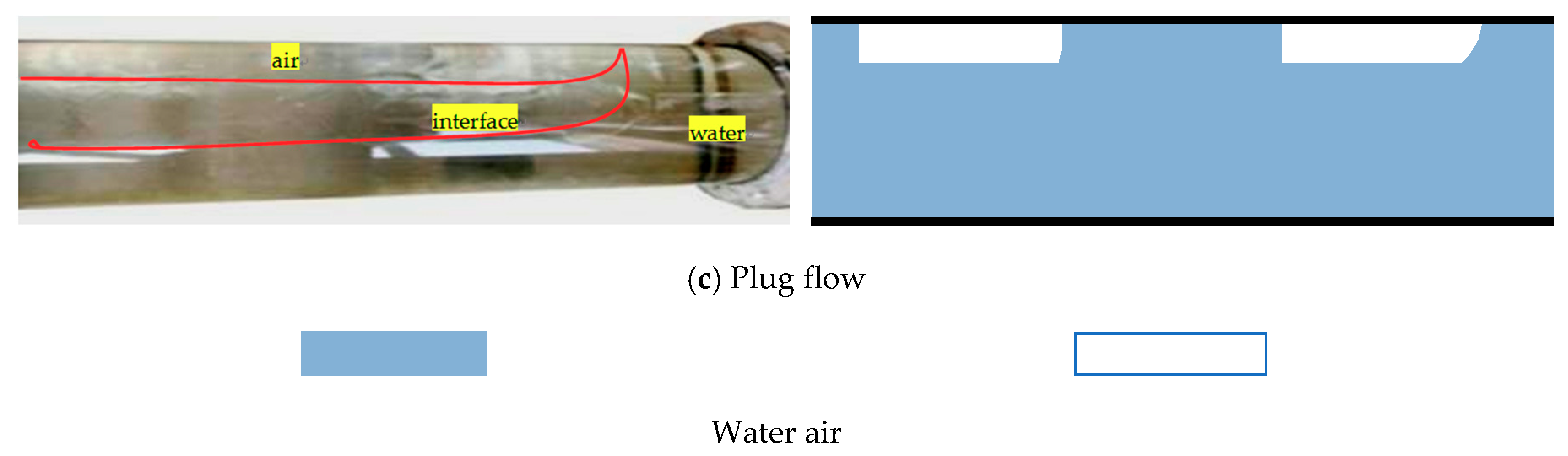
Plug flow (shown in Figure 3c): At the later stage of water filling, as the water lever in the pipe increases, due to the difference pipe bottom elevation, free-surface-pressurized water flow appears; that is, some parts of the flow are free surface (only a part of the cross-section of the pipe is filled), and other parts are pressurized (the whole cross-section of the pipe is filled),which also separates the air. Moreover, the air in the pipe is no longer a continuum. As a result, a plug flow is formed.

Generally, the main flow patterns occurred under water slow filling condition are the stratified smooth flow, the stratified wavy flow and the plug flow. The common feature of these three flow patterns is that there is a distinct stratification between water and air. Thus, establishing a water–air two-phase stratified model is appropriate for simulating the evolution of water flow and air in pipe, and a two-phase stratified flow model was attempted in the current study.

3.2. The Water–Air Interface

The water–air interface is determined jointly by the given flow rates, pipe parameters and physical properties of water and air [34], and many water–air two-phase stratified flow models are established by assuming the actual water–air interface as a simplified form [35]. In this section, a detailed discussion about assumption of water–air interface is given, and some processes in the established model are explained.

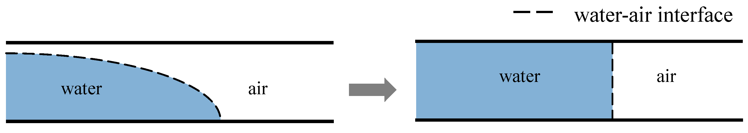
Generally, a pipe can be filled either with rapid or slow water filling. For rapid water filling, Wang et al. proposed an elastic column model for rapidly filling in the empty pipe, assuming that there is a vertical interface between the air and water [25]. This famous vertical interface assumption can be shown in Figure 4. In fact, Liou et al. proposed a criterion that such avertical interface assumption can be justified for pipe with relatively small diameter and rapid water flow velocity [36]. According to the experimental observation, there is an obvious horizontal stratified interface between water and air under water slow filling condition. Meanwhile, some other experimental and CFD model studies indicated that the pipe cross section is not entirely filled during the filling process, and thus, the vertical interface assumption does not match the real condition well and results in a decrease in the accuracy of the numerical model [37,38,39]. Meanwhile, Sampaio proposed a stratified water–air two phase flow model based on the assumption of smooth and horizontal water–air interface without considering the interfacial waves (shown in Figure 5) [18]. However, according to their simulation results, the model performed poorly along with increasing interface fluctuations. Therefore, assumptions of either vertical water–air interface or smooth-horizontal water–air interface are not suitable for the pipe under water slow filling in the current study. Furthermore, as indicted by Figueiredo et al. [40], when the interface presents significant curvature effects, there will be a non-negligible pressure difference between phases at any cross section, and the use of two pressures, one for each phase, may be necessary.

According to the observation (shown in Figure 3), the interface between water and air has obvious non-horizontal characteristics under water slow filling condition, for this reason, in the established model, the pressure gradient term for water and air have their respective expressions (see Equations (1b), (2b) and (11)). An algorithmic strategy for the water–air interface is presented: For every iteration calculation process, a judgment based on the Equation (3) is firstly made, according to this judgment, the fraction of water and air at each pipe cross section can be obtained, then due to this judgment, the iteration calculation process starts. This strategy is feasible under water slow filling condition.

3.3. Numerical Validation

The developed numerical model is validated based on the observed evolution of pressure in pipe and air velocity of air valves.

Table 3. The cells with measuring point ($\Delta x_i = 1m$, $C_d = 0.65$, T = 293 K).

Air Valve No.	Cell Location of Air Valves (i)	$\mathbf{Air}\mathbf{Valve}\mathbf{Diameter}{\mathit{d}}_{\mathit{v}}\left(\mathbf{mm}\right)$	$\mathbf{Air}\mathbf{Orifice}\mathbf{Area}{\mathit{A}}_{\mathit{v}}\left({10}^{-4}{\mathbf{m}}^2\right)$
1#	73	24	4.5216
2#	134	24	4.5216
3#	156	24	4.5216
4#	207	24	4.5216

shows the cells of measuring point with the space step $\Delta x_i$ = 1 m and the parameters of the air valve model.

3.3.1. The Pressure Evolution in Pipe during Water Slow Filling

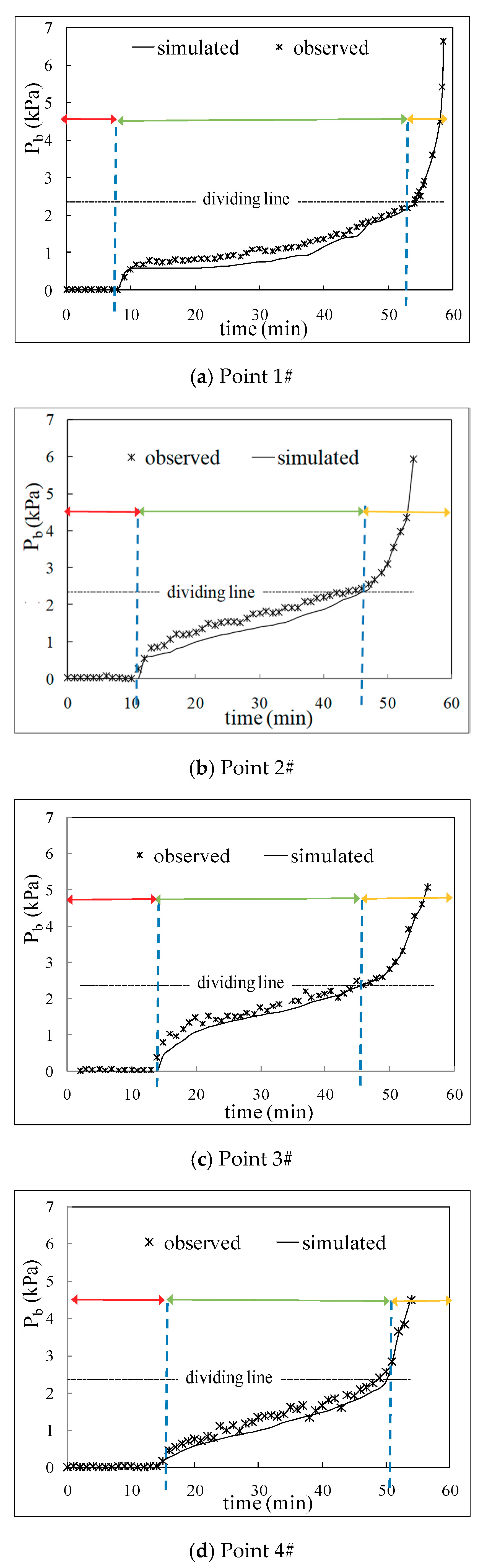
Theex perimental and numerical results of pressure evolution of pipe bottom at the four measuring points are shown in Figure 6. The developed model performed well in predicting the pressure evolution in the pipe, and the pressure for each measuring point varied in three distinct stages, namely the no-pressure, slowly increasing and rapidly increasing stage, which correspond to no water, free surface flows and pressurized flows, respectively. The water reached each measuring point at different times due to the varied distance to the upstream water tank, which resulted in the difference of pressure evolution among the four measuring points. However, the three stages at each measuring point are divided clearly.

It should be noted that the model performed well in predicting the pressure in the no-pressure and rapidly-increasing stage, while underestimating the pressure slightly in the slowly increasing stage for each measuring point. By inspecting the current model, the discrepancy may be due to the fact that only the water is taken into account in calculating the pressure in pipe. In fact, the pressure evolution in the pipe is affected by water and air when the two phases coexist in pipecrosssection. However, the influence of air is not considered, and the calculated pressure in pipe is equal to the water free-surface level $h$, so the numerical result is slightly smaller than the experimental data in the slowly increasing stage. In the rapidly increasing stage, the pressure evolution at each measuring point is only related to the water piezometric head, which resulted in good agreement between simulated pressure and the observation. In general, the developed model in this paper can reasonably predict the pressure evolution in the pipe.

3.3.2. The Air Velocity Evolution of Air Valves

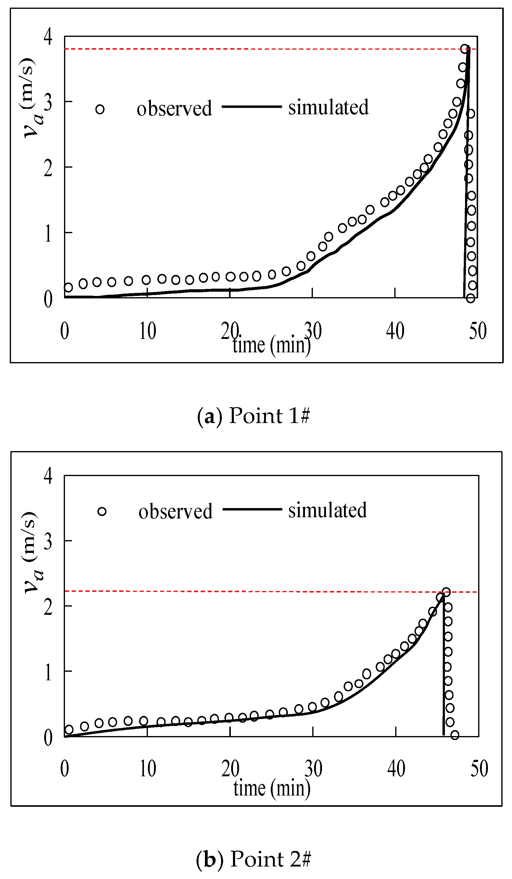
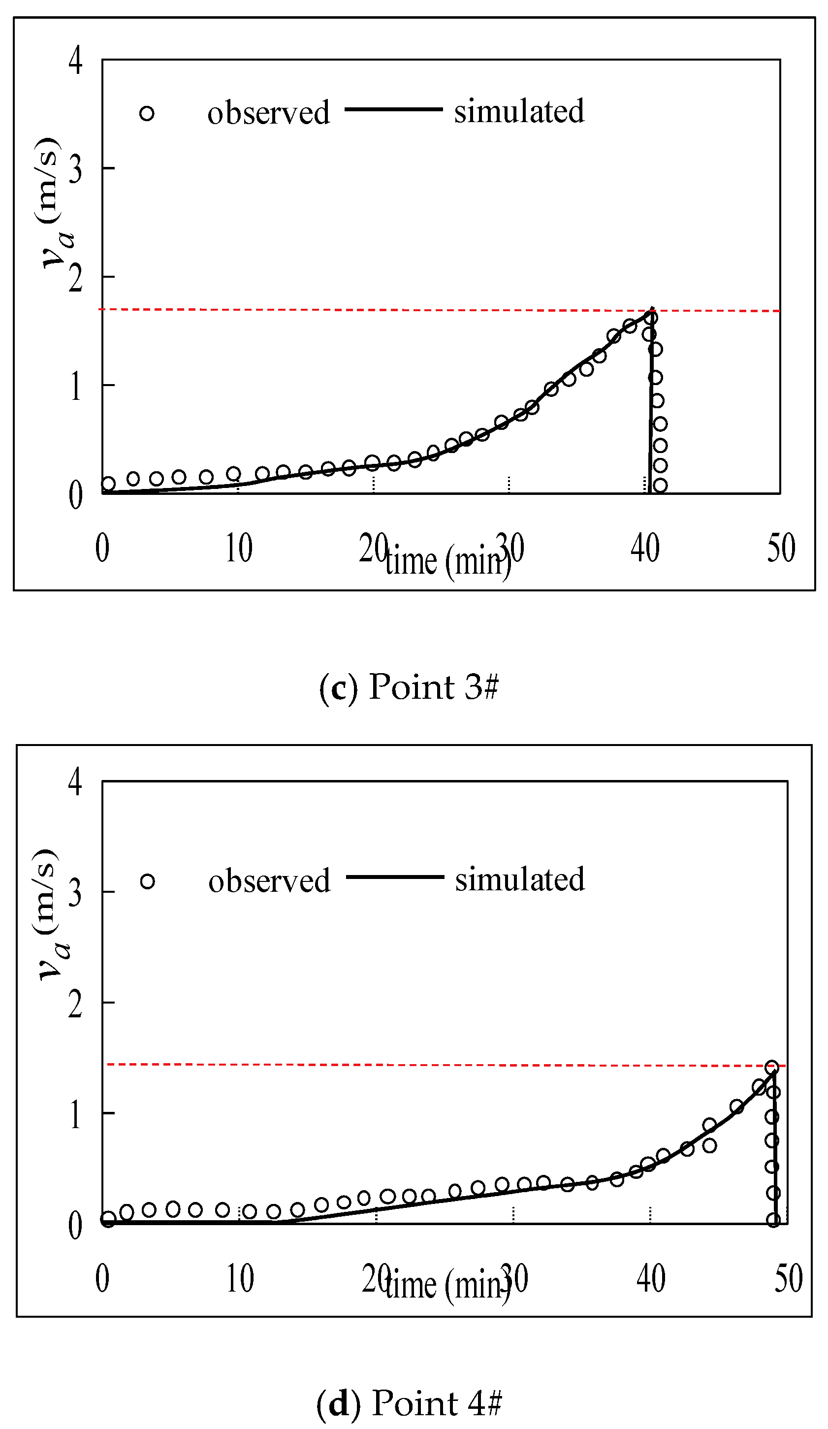
The observed and simulated air velocity evolution of each air valve are shown in Figure 7. When water enters the pipe, the air moves in pipe and expels from the air valves due to the pressure difference between inside and outside the pipe. The air velocity increases along with advance of water in pipe for each air valve and then up to the maximum at the end, when the pipe cross section is about to fill with water, finally droppingrapidly to zero in a very short moment. By comparing the observed and simulated air velocity, the numerical model can capture the air expelling process well, especially for the maximum air velocity. The maximum error between computed and measured maximum air velocity at the valves is about 5%. The numerical model gives sufficient accuracy and reasonable agreement with what is observed.

It is also noted that the deviation (e.g., the first ten minutes for the first air valves in Figure 7a) is still shown between the observed data and the numerical result. This error may be due to the compressibility and low inertia of the air; any external disturbance such as the upstream valve opening may cause the air to move. However, the developed model is intrinsically one-dimensional, which means all variables should be interpreted as being averages at the cross-sectional area of the pipe. As a result, these disturbances cannot be captured by the model in current study, which leads to the deviation. In general, the developed one-dimensional model is reasonable and applicable for simulating the air velocity evolution of air valves.

4. Summary and Conclusions

The main purpose of this article is to study the water filling and air expelling process of a pipe with multiple air valves under water slow filling condition and develop a fully coupled numerical model.

In the current study, a suitable two-pressure water–air two-phase stratified model is developed. For the model, the Saint-Venant and VANS equations are respectively used to describe the water and air in pipe, and the improved air valve model is incorporated in the VANS equations of air as the source term. The finite volume method and implicit dual time-stepping method are used in combination to solve the numerical model. Based on the observed varying water–air two-phase flow patterns in pipe under water slow filling condition, a detailed discussion about water–air interface is also given. In the current study, we firstly point out the inapplicability of the famous water–air vertical interface assumption and the smooth-horizontal water–air interface assumption and then present an algorithmic strategy. Meanwhile, due to the interface between water and air having obvious non-horizontal characteristics under water slow filling condition, the pressure gradient terms for water and air have their respective expressions in our model. The model is validated by using the experimental data of pressure evolution in pipe and air velocity evolution of air valves. The results show that although there are differences between the simulated result and the experimental data, the established model can reasonably simulate the pressure evolution of the pipe and the air expelling process, which is relatively consistent with the measured results. Thus, the established two-pressure two-phase stratified flow model is reasonable and applicable. This model will provide an effective method for the design of the air valve installation of the pipe and the verification of whether the existing air valve installation scheme is reasonable.

Finally, this model is developed for the water–air two phases flow patterns with distinct layering under water slow filling condition. The further experimental and numerical investigations are required for other flow patterns, and a more complete numerical model is expected to be established.

References

- Fuertes-Miquel, V.S.; López-Jiménez, P.A.; Martínez-Solano, F.J.; López-Patiño, G. Numerical modelling of pipelines with air pockets and air valves. Can. J. Civ. Eng. 2016, 43, 1052–1061. [Google Scholar] [CrossRef]
- Wu, Y.; Xu, Y.; Wang, C. Research on Air Valve of Water Supply Pipelines. Procedia Eng. 2015, 119, 884–891. [Google Scholar] [CrossRef]
- Bourdarias, C.; Ersoy, M.; Gerbi, S. A mathematical model for unsteady mixed flows in closed water pipelines. Sci. China Math. 2012, 55, 221–244. [Google Scholar] [CrossRef]
- Fernandez-Pato, J.; Garcia-Navarro, P. A pipeline network simulation model with dynamic transition between free surface and pressurized flow. Procedia Eng. 2014, 70, 641–650. [Google Scholar] [CrossRef]
- Garcia-Navarro, P.; Alcrudo, F.; Priestley, A. An implicit method for water flow modelling in canals and pipelines. J. Hydraul. Res. 1994, 32, 721–742. [Google Scholar] [CrossRef]
- An, H.; Lee, S.; Jin Noh, S.; Kim, Y.; Noh, J. Hybrid numerical scheme of Preissmann slot model for transient mixed flows. Water 2018, 10, 899. [Google Scholar] [CrossRef]
- Kerger, F.; Archambeau, P.; Erpicum, S.; Dewals, B.J.; Pirotton, M. An exact riemann solver and a godunov scheme for simulating highly transient mixed flows. J. Comput. Appl. Math. 2011, 235, 2030–2040. [Google Scholar] [CrossRef]
- Taitel, Y.; Lee, N.; Dukler, E. Transient gas-liquid flow in horizontal pipelines: Modeling the flow pattern transitions. AIChE J. 1978, 24, 920–934. [Google Scholar] [CrossRef]
- Wang, Z.; Gong, J.; Wu, C. Numerical Simulation of One-Dimensional Two-Phase Flow Using a Pressure-Based Algorithm. Numer. Heat Transf. Part A Appl. 2015, 68, 369–387. [Google Scholar] [CrossRef]
- Krasnopolsky, B.; Starostin, A.; Osiptsov, A.A. Unified graph-based multi-fluid model for gas–liquid pipeline flows. Comput. Math. Appl. 2016, 72, 1244–1262. [Google Scholar] [CrossRef]
- Shi, H.; Holmes, J.A.; Durlofsky, L.J.; Aziz, K.; Diaz, L.; Alkaya, B.; Oddie, G. Drift-Flux Modeling of Two-Phase Flow in Wellbores. SPE J. 2005, 10, 24–33. [Google Scholar] [CrossRef]
- Munkejord, S.T.; Evje, S.; Flåtten, T. The multi-stage centred-scheme approach applied to a drift-flux two-phase flow model. Int. J. Numer. Methods Fluids 2006, 52, 679–705. [Google Scholar] [CrossRef]
- Bestion, D. The physical closure laws in the CATHARE code. Nucl. Eng. Des. 1990, 124, 229–245. [Google Scholar] [CrossRef]
- Choi, J.; Pereyra, E.; Sarica, C.; Park, C.; Kang, J.M. An efficient drift–flux closure relationship to estimate liquid holdups of gas–liquid two-phase flow in pipelines. Energies 2012, 5, 5294–5306. [Google Scholar] [CrossRef]
- Tiselj, I.; Petelin, S. Modelling of Two-Phase Flow with Second-Order Accurate Scheme. J. Comput. Phys. 1997, 136, 503–521. [Google Scholar] [CrossRef]
- Issa, R.; Kempf, M. Simulation of slug flow in horizontal and nearly horizontal pipelines with the two-fluid model. Int. J. Multiph. Flow 2003, 29, 69–95. [Google Scholar] [CrossRef]
- Bonizzi, M.; Andreussi, P.; Banerjee, S. Flow regime independent, high resolution multi-field modelling of near-horizontal gas–liquid flows in pipelines. Int. J. Multiph. Flow 2009, 35, 34–46. [Google Scholar] [CrossRef]
- De Sampaio, P.A.B.; Faccini, J.L.H.; Su, J. Modelling of stratified gas–liquid two-phase flow in horizontal circular pipelines. Int. J. Heat Mass Transf. 2008, 51, 2752–2761. [Google Scholar] [CrossRef]
- Sondermann, C.N.; Baptista, R.M.; Bastos de Freitas Rachid, F.; Bodstein, G.C.R. Numerical simulation of non-isothermal two-phase flow in pipelines using a two-fluid model. J. Pet. Sci. Eng. 2019, 173, 298–314. [Google Scholar] [CrossRef]
- Vasconcelos, J.G.; Wright, S.J. Geysering generated by large air pockets released through water-filled ventilation shafts. J. Hydraul. Eng. 2011, 137, 543–555. [Google Scholar] [CrossRef]
- Liu, D.; Zhou, L.; Karney, B.; Zhang, Q.; Ou, C. Rigid-plug elastic-water model for transient pipe flow with entrapped air pocket. J. Hydraul. Res. 2011, 49, 799–803. [Google Scholar] [CrossRef]
- Zhou, L.; Liu, D.; Karney, B.; Zhang, Q. Influence of entrapped air pockets on hydraulic transients in water pipelines. J. Hydraul. Eng. 2011, 137, 1686–1692. [Google Scholar] [CrossRef]
- Zhou, L.; Liu, D.; Karney, B. Investigation of hydraulic transients of two entrapped air pockets in a water pipeline. J. Hydraul. Eng. 2013, 139, 949–959. [Google Scholar] [CrossRef]
- Wylie, E.B.; Streeter, V.L. Fluid Transients in Systems; Prentice Hall: Englewood Cliffs, NJ, USA, 1993. [Google Scholar]
- Wang, L.; Wang, F.; Karney, B.; Malekpour, A. Numerical investigation of rapid filling in bypass pipelines. J. Hydraul. Res. 2017, 55, 647–656. [Google Scholar] [CrossRef]
- Coronado-Hernández, Q.E.; Besharat, M.; Fuertes-Miquel, V.S.; Ramos, H.M. Effect of a Commercial Air Valve on the RapidFilling of a Single Pipeline: ANumerical and Experimental Analysis. Water 2019, 11, 1814. [Google Scholar] [CrossRef]
- Malekpour, A.; Karney, B.W. Spurious Numerical Oscillations in the Preissmann Slot Method: Origin and Suppression. J. Hydraul. Eng. 2016, 142, 04015060. [Google Scholar] [CrossRef]
- Liu, J.; Zhang, S.; Xu, D.; Bai, M.; Liu, Q. Coupled simulation and validation with fully implicit time scheme for free-surface-pressurized water flow in pipe/channel. Trans. Chin. Soc. Agric. Eng. (Trans. CSAE) 2017, 33, 124–130, (In Chinese with English abstract). [Google Scholar] [CrossRef]
- Shokri, V.; Esmaeili, K. Comparison of the effect of hydrodynamic and hydrostatic models for pressure correction term in two-fluid model in gas-liquid two-phase flow modeling. J. Mol. Liq. 2017, 237, 334–346. [Google Scholar] [CrossRef]
- LeVeque, R.J. Finite Volume Methods for Hyperbolic Problems; Cambridge University Press: Cambridge, UK, 2002. [Google Scholar]
- Zhang, S.; Xu, D.; Bai, M.; Li, Y.; Liu, Q. Fully Hydrodynamic Coupled Simulation of Surface Flows in Irrigation Furrow Networks. J. Irrig. Drain. Eng. 2016, 142, 04016014. [Google Scholar] [CrossRef]
- Belov, A.; Martinelli, L.; Jameson, A. A new implicit algorithm with multigrid for unsteady incompressible flow calculations. In Proceedings of the AIAA 33rd Aerospace Sciences Meeting, Reston, VA, USA, 9–12 January 1995. [Google Scholar]
- Jameson, A.; Yoon, S. Lower-upper implicit schemes with multiple grids for the Euler equations. AIAA J. 1987, 25, 929–935. [Google Scholar] [CrossRef]
- Picchi, D.; Poesio, P. A unified model to predict flow pattern transitions in horizontal and slightly inclined two-phase gas/shear-thinning fluid pipeline flows. Int. J. Multiph. Flow 2016, 84, 279–291. [Google Scholar] [CrossRef]
- Laanearu, J.; Annus, I.; Koppel, T.; Bergant, A.; Vučković, S.; Hou, Q. Emptying of Large-Scale Pipeline by Pressurized Air. J. Hydraul. Eng. 2012, 138, 1090–1100. [Google Scholar] [CrossRef] [Green Version]
- Liou, C.P.; Hunt, W.A. Filling of pipelines with undulating elevation profiles. J. Hydraul. Eng. 1996, 122, 534–539. [Google Scholar] [CrossRef]
- Hou, Q.; Tijsseling, A.S.; Laanearu, J.; Annus, I.; Koppel, T.; Bergant, A. Experimental investigation on rapid filling of a large scale pipeline. J. Hydraul. Eng. 2014, 140, 04014053. [Google Scholar] [CrossRef] [Green Version]
- Laanearu, J.; Hou, Q.; Annus, I.; Tijsseling, A.S. Water-column mass losses during the emptying of a large-scale pipeline by pressurized air. Proc. Est. Acad. Sci. 2015, 64, 8–16. [Google Scholar] [CrossRef]
- Tijsseling, A.S.; Hou, Q.; Bozkus, Z.; Laanearu, J. Improved one-dimensional models for rapid emptying and filling of pipelines. J. Press. Vessel Technol. Trans. ASME 2016, 138, 031301. [Google Scholar] [CrossRef] [Green Version]
- Figueiredo, A.B.; Baptista, R.M.; FreitasRachid, F.B.; Bodstein, G.C.R. Numerical simulation of stratified-pattern two-phase flow in gas pipelines using a two-fluid model. Int. J. Multiph. Flow 2017, 88, 30–49. [Google Scholar] [CrossRef]
Figure 1.
The pipe schematic layout of the experimental system.
Figure 2.
Configuration and its labeling.
Figure 3.
Water–air two-phase flow patterns recorded by high-speed cameras and their schematic diagram: (a) stratified smooth flow; (b) stratified wave flow; (c) plug flow.
Figure 4.
Water–air vertical interface assumption in Wang’s article [25].
Figure 5.
Vertical interface assumption in Sampaio’s article [18].
Figure 6.
The observed pressure evolution versus simulated pressure evolution based on the numerical models of four measuring points (the red, green and yellow double arrow lines indicate the no-pressure, slowly increasing and rapidly increasing stage, respectively): (a) measuring point 1#; (b) measuring point 2#; (c) measuring point 3#; (d) measuring point 4#.
Figure 7.
The observed air velocity versus simulated air velocity based on the numerical models of four measuring points (the redlines in each figure indicate the highest air velocity): (a) measuring point 1#; (b) measuring point 2#; (c) measuring point 3#; (d) measuring point 4#.