Changes in Physical Properties of Inland Streamwaters Induced by Earth and Atmospheric Tides

Abstract

Earth and atmospheric tides create oscillations in water parameters of inland rivers, mainly due to the similar behavior of groundwaters. Tidal oscillations of inland rivers were termed orthotides and were detected in fluctuations of water level and specific conductivity of some rivers. However, few things are understood about orthotides because of their recent discovery. Here, we show that orthotidal signals exist in streamwater temperature too. Wavelet and T_TIDE analyses are used to study streamwater temperature and specific conductivity. We found solar and lunar semidiurnal orthotides (S2 and M2) in Alapaha River (USA) water temperature and Wybong River (Australia) water specific conductivity with amplitudes of up to 0.6 °C and 11.3 µS/cm. We demonstrate that the tidal semidiurnal cycles have statistical significance and are caused by similar cycles in groundwater. Oscillations found in water temperature time series for some new moon time intervals have shapes that correlate with the gravitational tides. Diurnal and fortnightly tidal cycles were found and overlapped with other natural cycles with similar periodicities. The inclusion of more water parameters to the list of orthotidally sensitive parameters indicates the wider than expected environmental impact of the small periodic natural changes.

1. Introduction

Natural streamflow characteristics at small temporal scales are modulated by periodicities created by the Earth’s rotation and position relative to some celestial bodies (sun and moon) [1,2]. The most persistent and easily measurable periodicity is represented by the diurnal cycle (caused by the day/night change), which is observed in numerous physical/chemical streamwater parameters (such as water level [3] or temperature [4]), sometimes due to their interdependence [5], and is imposed mainly through the cyclic changes in air temperature and catchment evapotranspiration [6]. This diurnal cycle is present in groundwater too, where it is sometimes mixed with cycles that are caused by inland tides [7,8]. Gravitational tides generate earth and atmospheric tides, which create periodic fluctuations in groundwater level at various temporal scales, such as diurnal and semidiurnal; the main tidal constituents of the lunar and solar influences on groundwater are M2, S2, N2, K1, and O1 [9,10]. Not only the inland groundwater level/flow but also the electric conductivity and pH of groundwaters records tides, according to a recent study [11]. Radon concentrations in groundwater are useful for identifying some groundwater oscillations as the effect of earth tides [12].

Recent studies found semidiurnal tidal oscillations in rivers that are far from sea tides [13,14]. The rivers in these studies were analyzed at reaches that are not tidal, meaning that ocean tides do not propagate inland towards the monitoring points due to the high distances from the shoreline (tens or hundreds of km) and especially due to the terrain elevation, which is higher than the highest ocean tide. These oscillations are caused by tidal signals transferred from groundwater into rivers and were termed orthotides in order to differentiate them from the river tides, found in coastal areas [14]. Orthotides were observed in fluctuations of water level and electrical conductivity of some rivers across the globe [13,14,15,16,17]. Because of the water exchanges between groundwaters and rivers, river diurnal profile is sometimes enriched with a second(ary) peak due to the semidiurnal tidal periodicities in groundwater. Double-peaked diurnal evolutions were rarely observed (being considered a noisy behavior) on rivers with weak or no anthropogenic impact and cannot be attributed to natural transient (such as stormwater runoff) or unphased processes when they occur for multiple consecutive weeks and have strong correlations with similar evolutions in environments (such as the groundwater) that impact the streamwater. Groundwater level oscillations are also caused by atmospheric tides, which have high temporal variability within a day (2–3 h) [12] and generate different outputs when combined with earth tides. After the groundwater signals are exported into rivers, a certain orthotidal streamwater behavior can be detected mainly if a semidiurnal signal is present; the diurnal cycle is not useful due to the much stronger influence of the solar thermal factor [13,17]. The findings in this study add more details to the lunar tidal influence that was analyzed at the monthly scale [18].

Due to the numerous variations that occur continuously in watersheds, the orthotidal oscillations of rivers tend to be altered, overwritten, or completely diminished under our limit of detection. As result, finding rivers with easily measurable orthotides is still an important discovery. Such rivers allow for understanding some of the variations that were previously included in the general category of noises. The awareness of the existence of orthotidal oscillations might help reduce the uncertainty of some models used in hydrological sciences. The inclusion of orthotides in various analyses has the potential to increase the precision of forecasts.

The main objective of this study is to provide direct evidence that orthotides exist in Alapaha River water temperature time series and in Wybong River specific conductivity. This is possible due to the local natural favorable conditions and to the newer instruments in the field that have an increased resolution, useful for detecting smaller natural oscillations. Specific objectives are to detect semidiurnal oscillations in the streamwater time series of the studied sites; to find correlations with the gravitational, groundwater, and atmospheric tides; and to quantify the impact of each factor on the observed river water oscillations based on the characteristics of the tidal constituents.

This study is structured in three parts as follows: (1) an analysis of orthotides in Alapaha River by using river, groundwater, atmospheric, and gravitational data—analysis focused on streamwater temperature; (2) a similar analysis of Wybong River—analysis focused on streamwater specific conductivity; and (3) an analysis of semidiurnal oscillations detected in the time series of multiple parameters of Suceava River.

2. Materials and Methods

Streamwater data analyzed in this study were collected within various monitoring networks from 1993 until 2018 and represent rivers at gauges in nontidal reaches (

Table 1. Details of the studied sites and parameters.

No.	Monitoring Point	Latitude, Longitude	Elevation (m a.s.l.) *	Parameters	Time Interval
USA
1	USGS 02317500 ALAPAHA RIVER AT STATENVILLE, Georgia	30°42′14” N, 83°02′00” W	23	level/discharge	2007–2018
				temperature	2016–2018
2	USGS 02317620 ALAPAHA RIVER NEAR JENNINGS, Florida	30°35′53” N, 83°04′24” W	19	level/discharge	2007–2018
				temperature	2017–2018
				electrical conductivity	2017–2018
3	USGS 304949083165301 19E009 (Valdosta, Upper Floridan Aquifer), Georgia	30°49′51” N, 83°16′58” W	65	level	2007–2018
Australia
4	WYBONG CREEK AT MANOBALAI—210147, New South Wales	32°10′57” S, 150°39′39” E	172	level/discharge	2010–2018
5	WYBONG CREEK AT WYBONG—210040, New South Wales	32°16′9” S, 150°38′10” E	145	level/discharge, electrical conductivity	1993–2018
				temperature	1999–2018
6	GW080434.1.1 (Wybong Bridge, Wybong alluvial aquifer), New South Wales	32°12′4” S, 150°22′18” E	148	level	2003–2018
				temperature	2007–2018
Romania
7	SUCEAVA RIVER AT MIHOVENI, Suceava	47°40′53” N, 26°11′60” E	280	level, temperature, electrical conductivity, dissolved oxygen, pH, ORP	2018

* Datum: USA—NAVD88/NGVD29, Australia—AHD, Romania—WGS84.

). Water data were collected from United States Geological Survey (USA—https://waterdata.usgs.gov/nwis/), Office of Water of New South Wales (Australia—https://realtimedata.waternsw.com.au/water.stm) and a network of University of Suceava (Romania—http://water.usv.ro). Climate in the studied sites is variable from semiarid (Wybong) or humid subtropical (Alapaha) to temperate (Suceava), but the wettest season is the warm season; the average yearly sum of precipitation ranges from 600 to 1200 mm, while the average annual temperature ranges from 8 °C to 20 °C. Streamwater data are from nontidal reaches and areas with no significant human impact on environment. The average discharges are 0.6 m³/s for Wybong Creek, 17 m³/s for Suceava River, and 30 m³/s and 37 m³/s for Alapaha River at Statenville and Jennings, respectively. Groundwater values in this study represent the distance to water level in meters below the topographic surface. Data used in various analyses have a 15-min sampling frequency. Atmospheric pressure is mean sea level pressure of hourly frequency (upsampled to 15 min) from Valdosta and Tamworth airports, Automated Surface Observing System (ASOS) network (http://mesonet.agron.iastate.edu/request/download.phtml).

We used the “smooth” function in MATLAB with a moving average filter—the span was set differently depending on the level of noise in time series: time series of USA used a span of 11 values (out of 96, which represents a day length), while time series in Australia and Romania used a span of 3 values. The additive decomposition used for the alternate detrending method was computed with XLSTAT with a period of one day.

The continuous wavelet transform analysis was performed according to the methodology of Torrence and Compo [19] and of Ng and Chan [20] (the rectified power spectrum). It used Morlet as the mother wavelet. The wavelet coherence (WTC) analysis used the software provided by Grinsted et al. [21]. The high-power areas on scalograms surrounded by thick, black lines represent periods tested against the AR1 red noise (0.95 confidence level).

The Morlet wavelet is a nonorthogonal wavelet that is frequently used in the analysis of time series in geosciences [21] and is defined as follows:

$${\psi }_0\left(\eta \right)={\pi }^{-\frac{1}{4}}{e}^{i{\omega }_0\eta }{e}^{-\frac{1}{2}{\eta }^2},$$

(1)

where ω₀ and η are dimensionless frequency and time, respectively. For ω₀ = 6, the Fourier period is almost equal to scale, meaning that this frequency offers a balance between time and frequency localization [21]. The continuous wavelet transform of a time series X is defined as follows:

$$W_n^X\left(s\right)=\sqrt{\frac{\delta t}{s}}{\displaystyle \sum }_{n^{\prime }=1}^N{x}_{n^{\prime }}{\psi }_0\left[\left(n^{\prime }-n\right)\frac{\delta t}{s}\right],$$

(2)

where s is the wavelet scale, δt is the time step, and n represents the localized time index. According to Torrence and Webster [22] and Grinsted et al. [21], the wavelet coherence of the time series X and Y can be written as follows:

$$R_n^2\left(s\right)=\frac{{\left|S\left(s^{-1}{W}_n^{XY}\left(s\right)\right)\right|}^2}{S\left(s^{-1}{\left|W_n^X\left(s\right)\right|}^2\right)\times S\left(s^{-1}{\left|W_n^Y\left(s\right)\right|}^2\right)},$$

(3)

where $R=\sqrt{X^2+Y^2}$ and S represents a smoothing operator that has to be chosen depending on the wavelet used [21]. This formula indicates a localized correlation coefficient in time and frequency space.

Only raw data were included in the T_TIDE analysis (T_TIDE is a software specialized in finding details—such as amplitude and phase—of the known tidal constituents [23]). Because this software was intended for oceanic tides, K1 means mainly S1 for inland rivers (The software uses similar frequencies for both constituents; more than that, S1 in rivers is less stable than a tidal constituent and has a slightly variable period.).

Synthetic gravity tides were computed by using WPARicet (French Polynesia, Iles du Vent, Papeete, French Polynesia) (inputs: Tamura 1200 potential [24] and NAO99 ocean tide and non-hydrostatic/inelastic Earth models [25]) and ETERNA3.4 (French Polynesia, Iles du Vent, Papeete, French Polynesia) (for temporal evolution) softwares.

3. Results and Discussion

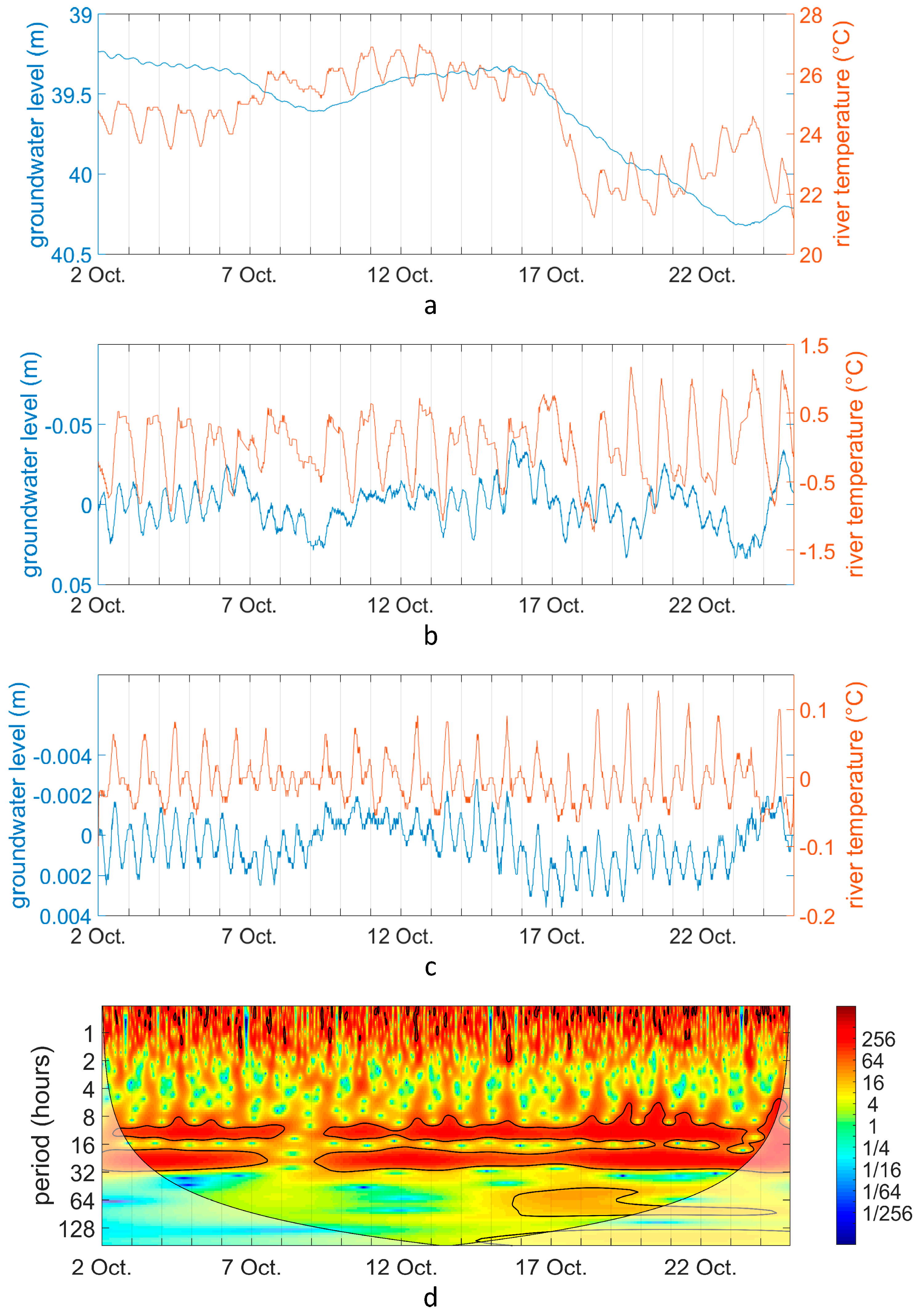
Water temperature of Alapaha River, a tributary of Suwannee River, has diurnal and semidiurnal oscillations that are easily detectable during multiple periods consisting of consecutive days. Selected examples are October 2017 (23 days; Figure 1a), October–December 2016 (57 days), August–September 2017 (30 days), December–February 2018 (59 days), and September–November 2018 (67 days) (Supplementary Figures S1–S4a). Figure 1 indicates that there are similarities in the temporal evolution of Alapaha River temperature and groundwater level, seen as small semidiurnal oscillations (Figure 1a). These oscillations can be better observed if the trends and oscillations with a period greater than a day are removed from the selected time series. This removal can be done through various techniques, and the following were applied in this study: differencing (Figure 1b) and additive decomposition (Figure 1c). The raw time series were also used for a continuous wavelet analysis, which generated a scalogram (Figure 1d), which displays the strength of a periodicity with red colors. The thick, black lines delineate time intervals where the detected periodicities have very low chances (<0.05%) to be red noise (probability tested through a Monte Carlo test). The diurnal cycle is caused by the input of solar heat during daytime in the river catchment, while the semidiurnal fluctuations follow the tidal pattern observed in groundwater (positive correlation). A comparison of the detrended time series of groundwater level and river temperature shows quasi-synchronous semidiurnal oscillations in both environments (Figure 1b,c; Supplementary Figures S1–S4b,c), with the observation that those in groundwater are more regular and are not marked by a strong diurnal cycle, which is very prominent in streamwaters due to the undelayed/direct contact with the atmosphere. Wavelet transform analyses indicate statistically significant (0.95) diurnal and semidiurnal signals in the selected river temperature time series (the red bands of ~12 and 24 h periods; Figure 1d and Supplementary Figures S1–S4d; tested against the AR1-type red noise). The wavelet coherence (WTC) analysis confirms the almost in-phase evolution (arrows pointing right) of the semidiurnal variations in groundwater level and streamwater temperature (Supplementary Figure S5).

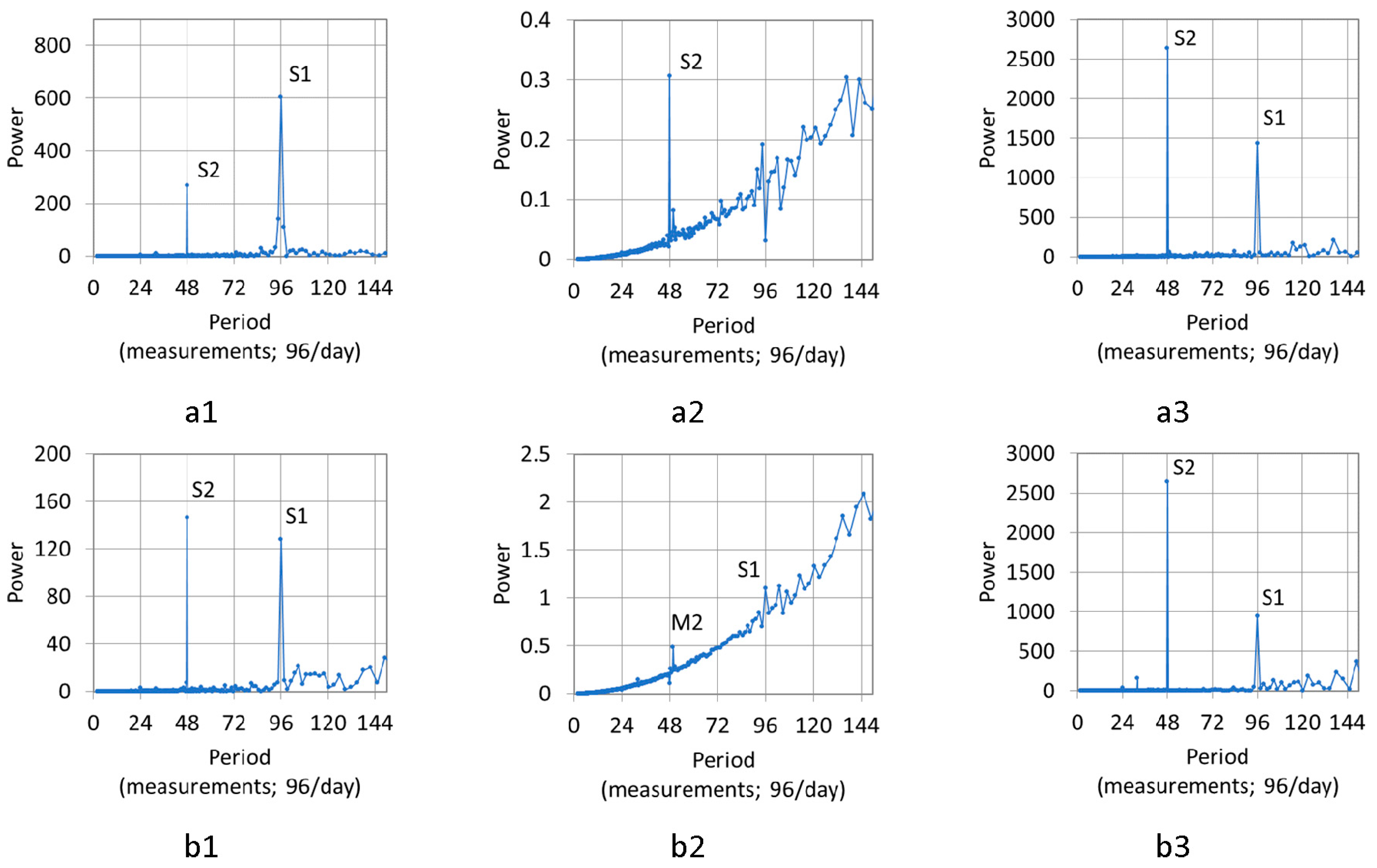
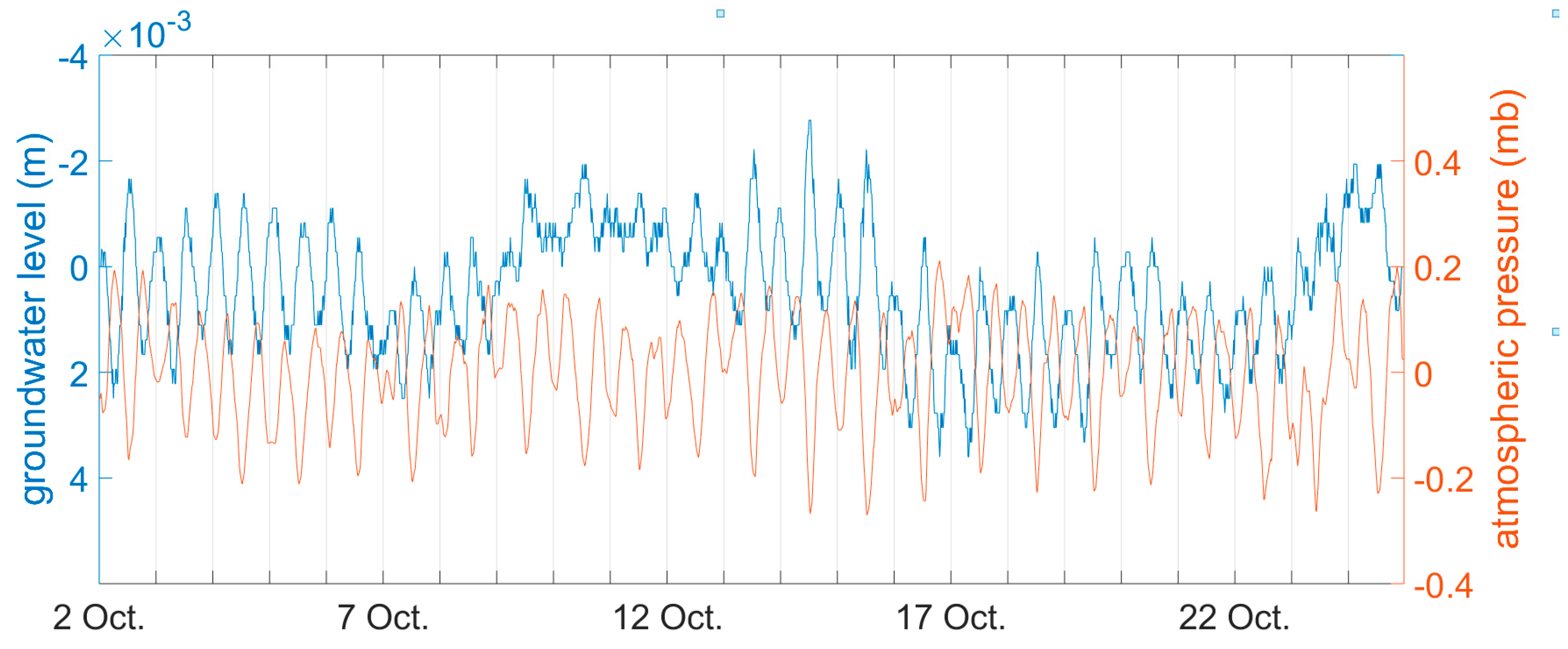
The Fourier analyses of river temperature, groundwater level, and atmospheric pressure in Alapaha area (Statenville–Valdosta) reveals similar periodicities in all environments (Figure 2, Supplementary Figure S6). Figure 2 reveals the power of the diurnal and semidiurnal signals in the selected environments. Significant signals are displayed as peaks that separate from the surrounding noise, e.g., S2 has a period of 48 measurements, meaning 2 cycles per day because a day contains 96 measurements (the sampling frequency is 15 min). River temperature is dominated by the solar diurnal (S1) cycle and has a secondary solar semidiurnal (S2) cycle, but an inverse case can also occur (Figure 2b1). Signals in groundwater level are S2, M2 (lunar semidiurnal), and S1, while the atmospheric pressure records a clearly dominant S2 over the weaker thermo-tidal S1. There is an antiphase relationship between atmospheric pressure and groundwater level at Valdosta (Figure 3), indicating the modulation of groundwater level by atmospheric tides. Also, due to the smaller amplitudes of the semidiurnal oscillations (than those of the diurnal cycle), these oscillations are often buried in noise and the significant areas of the semidiurnal band on scalograms are less extended than those of the diurnal band (areas surrounded by a thick, black line; Figure 1d, Supplementary Figures S1–S4). Previous studies also highlighted the shadowing effect of the diurnal cycles [13,17], which impedes the full extraction of the semidiurnal cycles through methods such as differencing or detrending. Other methods for removing diurnal cycle, like high pass filtering, are only in some cases successful (Supplementary Figure S7) but lead to increased data artificialization and were avoided in this study.

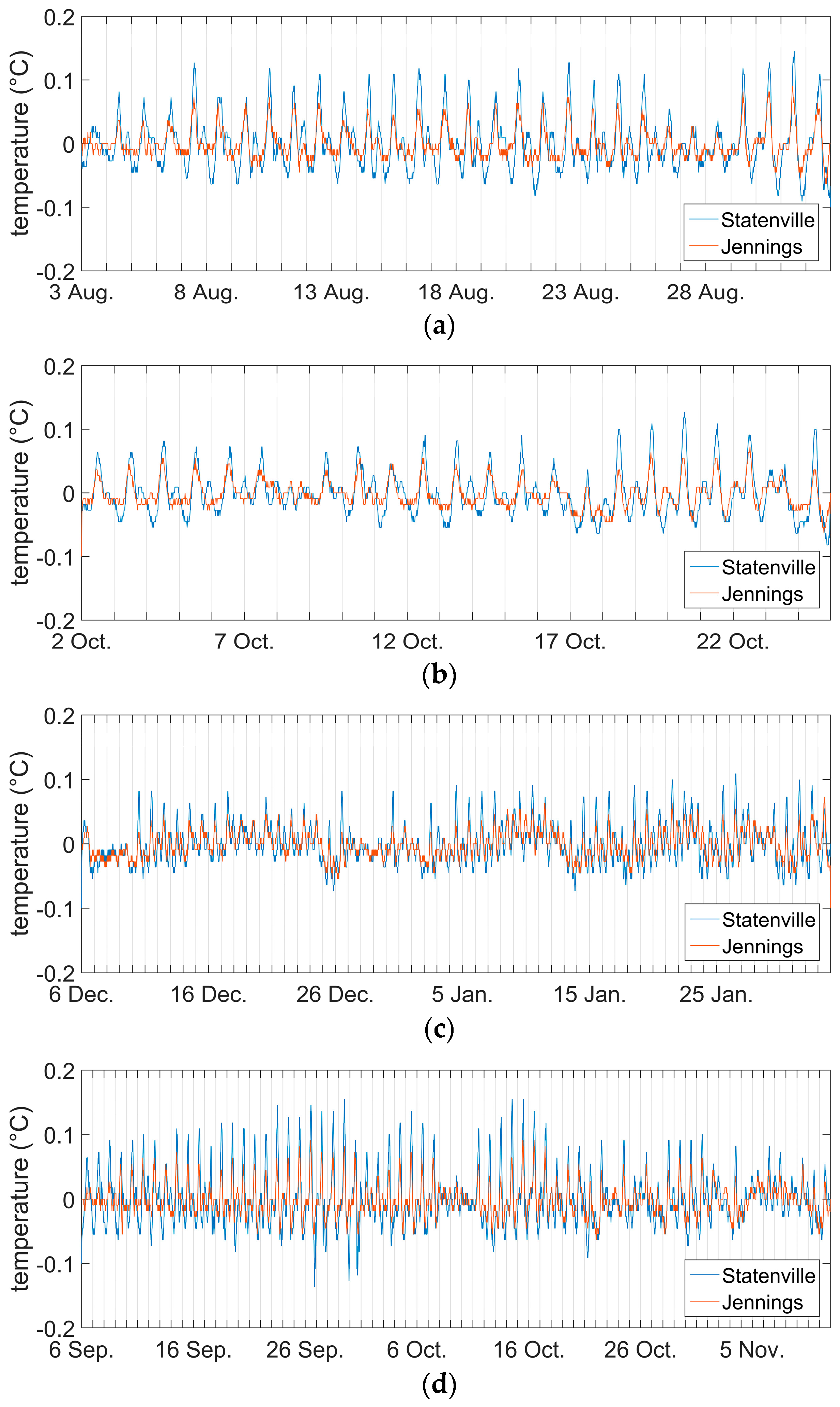
Oscillations found in Alapaha River at Statenville (Georgia) are also present 12.5 km downstream (straight line) at Jennings (Florida). Here, shorter time series of water temperature were available and the detected semidiurnal oscillations have smaller amplitudes than at Statenville (Figure 4), which might make them more sensible to being erased by other environmental signals/noises and harder to measure.

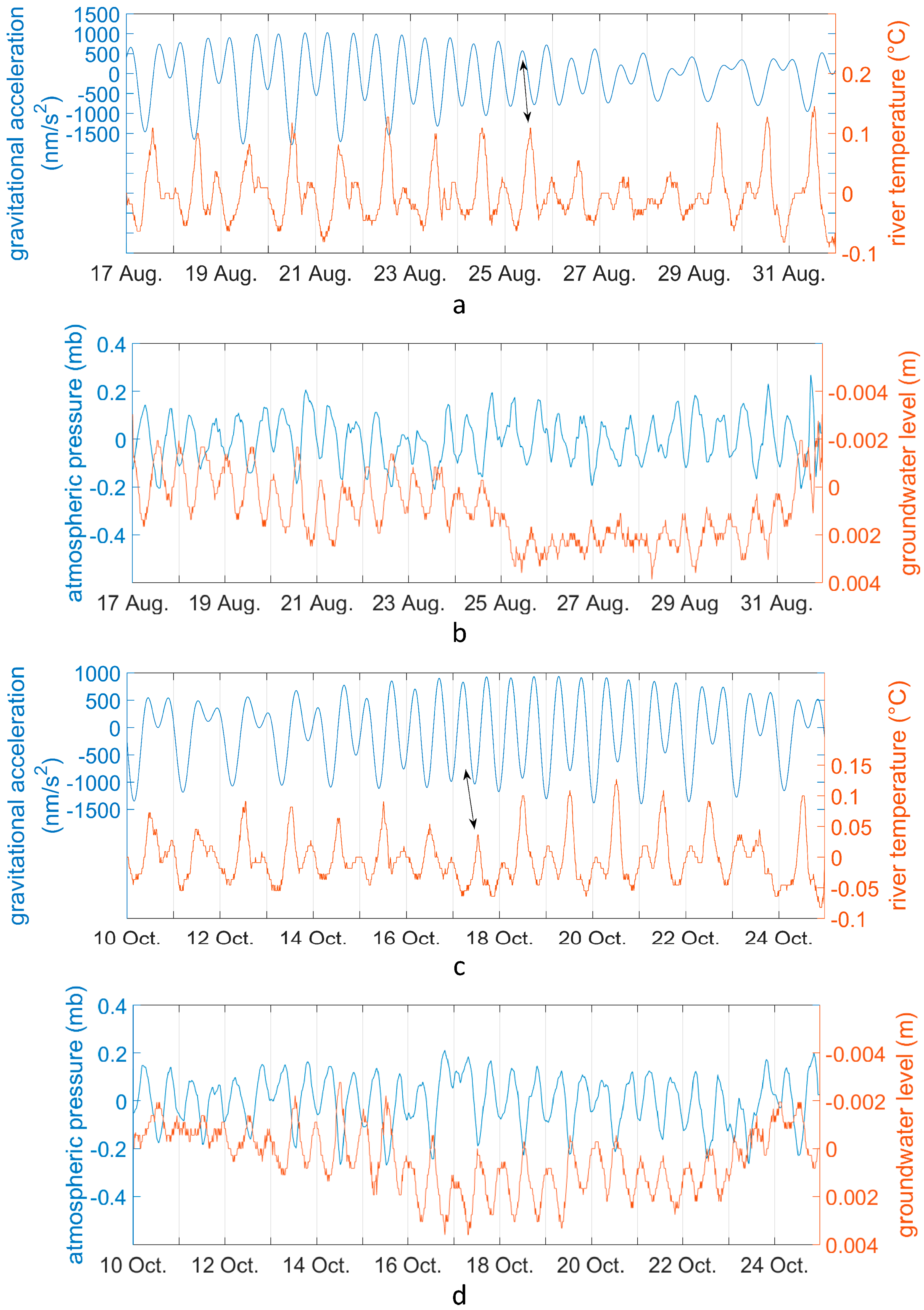
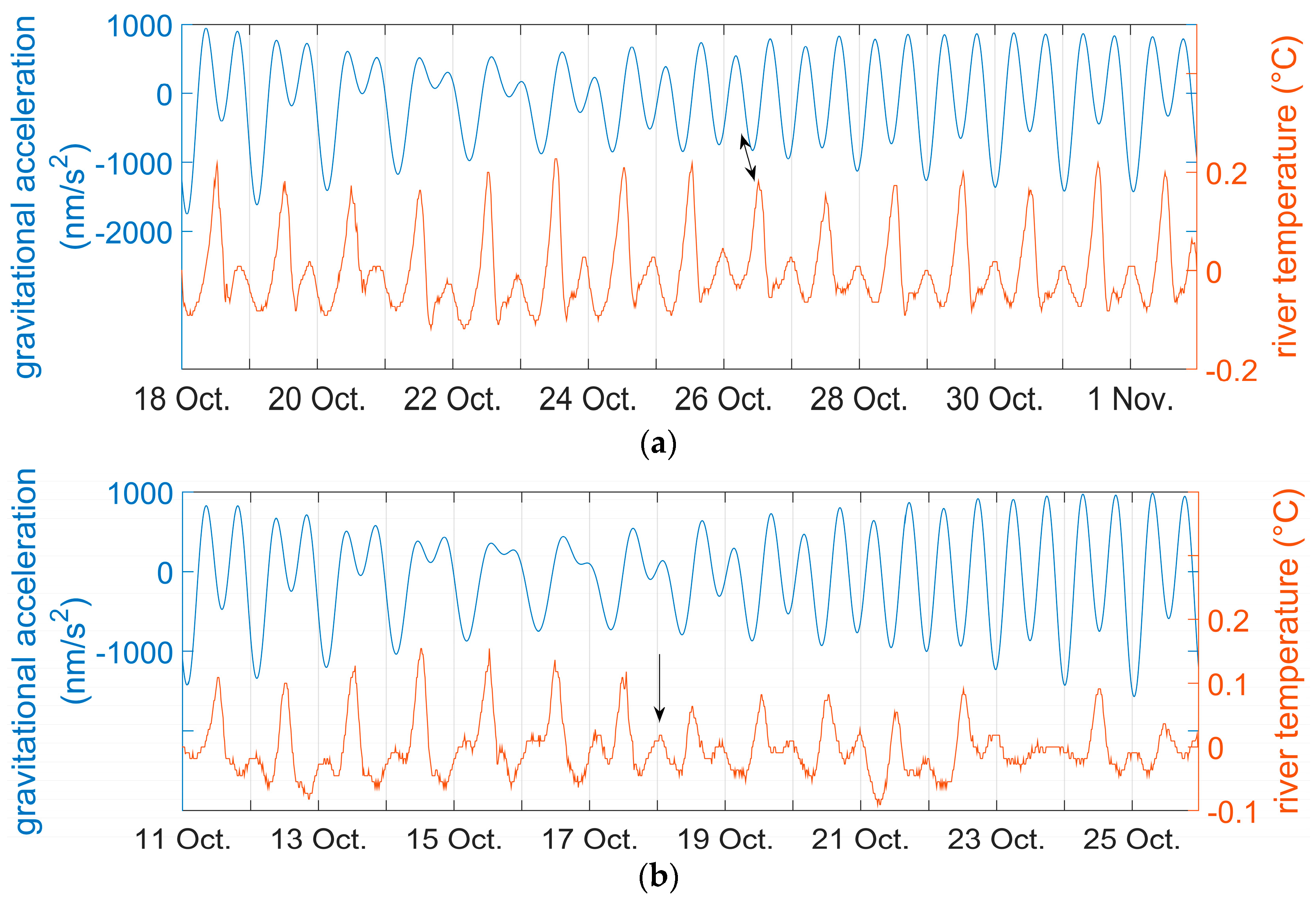
Even if the solar diurnal and semidiurnal signals of atmospheric origin are the dominant forces that modulate the orthotidal behavior of Alapaha River, there are also important fluctuations that are directly related to the similar evolution of the earth tides (Figure 5). Figure 5 compares the semidiurnal signals in river temperature, groundwater level, atmospheric pressure, and gravitational acceleration time series in order to prove that oscillations induced by earth tides in groundwater are then transmitted from groundwater into river. A delayed response (a couple of hours) can be sometimes observed in river temperature as result of changes in variations of the gravitational acceleration. More specifically, during the new moon period, the moment of producing the semidiurnal peak that belongs to 2 (instead of 1) diurnal pairs of peaks/valleys in gravity causes a dominant diurnal peak in river temperature (Figure 5a,c and Figure 6a); this latter peak is unpaired when considering the diurnal cycles previous and next to its occurrence. A similar evolution in groundwater can be easily observed (Figure 5d) but lacks in the atmospheric pressure time series (Figure 5b,d), proving the origin of the unpaired peak in the fluctuations of the earth tides. Not only the syzygy but also the quadrature imply an earth tide impact on river temperature (through groundwater fluctuations); the specific evolution of the gravitational acceleration approximately during quadratures can also create an unimpaired peak in streamwater temperature, but this peak is a minor one when compared to neighbor peaks in diurnal cycles (Figure 6b).

In order to have a more precise analysis of the tidal harmonics in streamwater, we used the T_TIDE software and, in addition to the solar constituents detected with the FFT, we found lunar and lunisolar tidal components (MSF, O1, K1, and M2) in time series with a length of 15 days (Figure 5 and Figure 6a). These new time series were cut from the longer data sets, discussed previously, in sectors with semidiurnal oscillations that are easily detectable at a visual inspection of the raw data and have a length of 15 days in order to include a fortnightly period. Significant M2 was found at both gauges from Alapaha catchment and in groundwater (

Table 2. Details of tidal constituents found in the Alapaha-Valdosta area by using T_TIDE (tidal amplitude and phase with 95% CI estimates; phases at central time; bold for semidiurnal signals with signal to noise ratio equal to or greater than 2).

Time Interval	Site-Parameter	Tidal Component	Period (h)	Amplitude *	Amplitude Error *	Phase (°)	Phase Error (°)	Signal to Noise Ratio
17–31 August 2017	Statenville—streamwater temperature	MSF	354	1.0118	0.172	293.08	9.76	34
		O1	25.82	0.2013	0.142	253.11	42.61	2
		S1/K1	24/23.93	0.5116	0.145	111.72	18.71	12
		M2	12.42	0.0317	0.081	88.35	125.88	0.15
		S2	12	0.3059	0.097	107.56	17.67	9.9
	Jennings—streamwater temperature	MSF	354	0.8527	0.066	298.19	4.39	170
		O1	25.82	0.1224	0.059	194.87	29.7	4.3
		S1/K1	24/23.93	0.3421	0.063	94.01	10.65	30
		M2	12.42	0.0408	0.034	327.71	46.72	1.4
		S2	12	0.1493	0.033	90.18	15.28	20
	Valdosta—groundwater level	MSF	354	0.6332	0.02	293.4	1.78	970
		O1	25.82	0.0297	0.02	88.58	38.65	2.3
		S1/K1	24/23.93	0.0282	0.019	260.08	41.26	2.2
		M2	12.42	0.021	0.008	269.03	24.65	6.3
		S2	12	0.0196	0.01	104.12	28.25	4.1
10–24 October 2017	Statenville—streamwater temperature	MSF	354	2.1746	0.152	257.29	4.1	200
		O1	25.82	0.1302	0.129	330.74	70.7	1
		S1/K1	24/23.93	0.3621	0.15	102.9	24.61	5.8
		M2	12.42	0.0151	0.038	111.01	174.52	0.16
		S2	12	0.2973	0.062	108.66	10.7	23
	Jennings—streamwater temperature	MSF	354	2.2924	0.1	258.79	2.21	530
		O1	25.82	0.082	0.075	178.76	58.84	1.2
		S1/K1	24/23.93	0.1865	0.09	90.07	29.37	4.3
		M2	12.42	0.0724	0.038	315.25	35.46	3.6
		S2	12	0.1807	0.04	94.5	10.88	20
	Valdosta—groundwater level	MSF	354	0.4659	0.01	289.05	1.2	2300
		O1	25.82	0.0125	0.008	101.08	40.33	2.4
		S1/K1	24/23.93	0.0094	0.009	260.8	60.54	1.2
		M2	12.42	0.0058	0.004	237.32	41.01	2.6
		S2	12	0.0134	0.004	112.42	19.24	11
11–25 October 2018	Statenville—streamwater temperature	MSF	354	1.6057	0.256	332.98	8.98	39
		O1	25.82	0.336	0.256	129.78	40.3	1.7
		S1/K1	24/23.93	0.3991	0.254	99.56	34.11	2.5
		M2	12.42	0.0782	0.046	246.26	34.95	2.9
		S2	12	0.3375	0.043	109.23	8.31	62
	Jennings—streamwater temperature	MSF	354	1.397	0.155	335.3	6.3	81
		O1	25.82	0.2845	0.152	94.31	32.26	3.5
		S1/K1	24/23.93	0.2056	0.153	100.97	37.59	1.8
		M2	12.42	0.0753	0.049	228.89	39.15	2.4
		S2	12	0.1884	0.048	87.7	13.93	15
	Valdosta—groundwater level	MSF	354	0.1404	0.003	354.86	1.32	1900
		O1	25.82	0.0053	0.003	83.9	32.84	2.9
		S1/K1	24/23.93	0.0012	0.002	80.98	133.03	0.36
		M2	12.42	0.0022	0.001	50.33	25.12	7.8
		S2	12	0.0081	0.001	127.21	5.59	83
18 October–1 November 2016	Statenville—streamwater temperature	MSF	354	1.7623	0.172	189.37	5.55	100
		O1	25.82	0.0533	0.126	195.39	141.16	0.18
		S1/K1	24/23.93	0.8898	0.17	105.55	10.56	27
		M2	12.42	0.0508	0.055	104.83	74.27	0.84
		S2	12	0.6377	0.061	88.5	4.58	110
	Valdosta—groundwater level	MSF	354	0.2263	0.01	263.02	2.57	470
		O1	25.82	0.0151	0.009	93.1	34.84	2.6
		S1/K1	24/23.93	0.0086	0.009	246.6	65.7	0.84
		M2	12.42	0.0044	0.005	283.26	67.1	0.88
		S2	12	0.0137	0.005	109.94	19.57	8.3

* Units in °C for streamwater and in m for groundwater.

).

S2 usually has higher amplitude and SNR (signal to noise ratio) than M2 in both streamwater and groundwater. The highest measured amplitude of S2 is ~0.64 °C, while the correspondent value for M2 is ~0.08 °C. The lunisolar synodic fortnightly cycle (MSF) was also detected in these case study time series (the maximum measured amplitude is ~2.29 °C) and is significant in longer time series too in both groundwater and surfacewater time series (However, even if it has high SNR, the MSF signal could also include other long-wave nontidal natural cycles (e.g., changes in synoptic conditions) and is not taken into account as a principal proof—a similar case is for the diurnal cycle, which may include simultaneously S1, O1, and K1.).

The groundwater level recorded at Valdosta (and compared with Alapaha River temperature) is from a well completed in the Upper Floridan Aquifer. The potentiometric surface of this karstic aquifer indicates that the groundwater flows on a NW–SE direction from Lowndes county (Valdosta) towards Echols county (Statenville) [26]. In the Statenville–Jennings area, the Upper Floridan Aquifer is covered by the Upper Semiconfining Unit of Hawthorn Group and the surficial aquifer of the Coastal Plain. In the southern part of this area, the Suwannee limestone of the Floridan Aquifer crops along a northern extension of Cody Escarpment in streambeds (the scarp separates the Northern Highlands region from the Gulf Coastal Lowlands). As the Floridan Aquifer is thinly confined or unconfined in the study area, direct or indirect discharge–recharge events between this aquifer and Alapaha River can occur. A similar case is for the Floridan Aquifer at Valdosta, where it is recharged by surface waters [27], which are then partly redirected towards Statenville–Jennings. The transmissivity of the Upper Floridan Aquifer in this area has values of over 900 m²/day (in the western parts of Echols and Hamilton counties, which are surrounded by areas with much lower transmissivities of around 140–185 m²/day) [28], and this may also explain the efficient groundwater-streamwater export of the tidal signals.

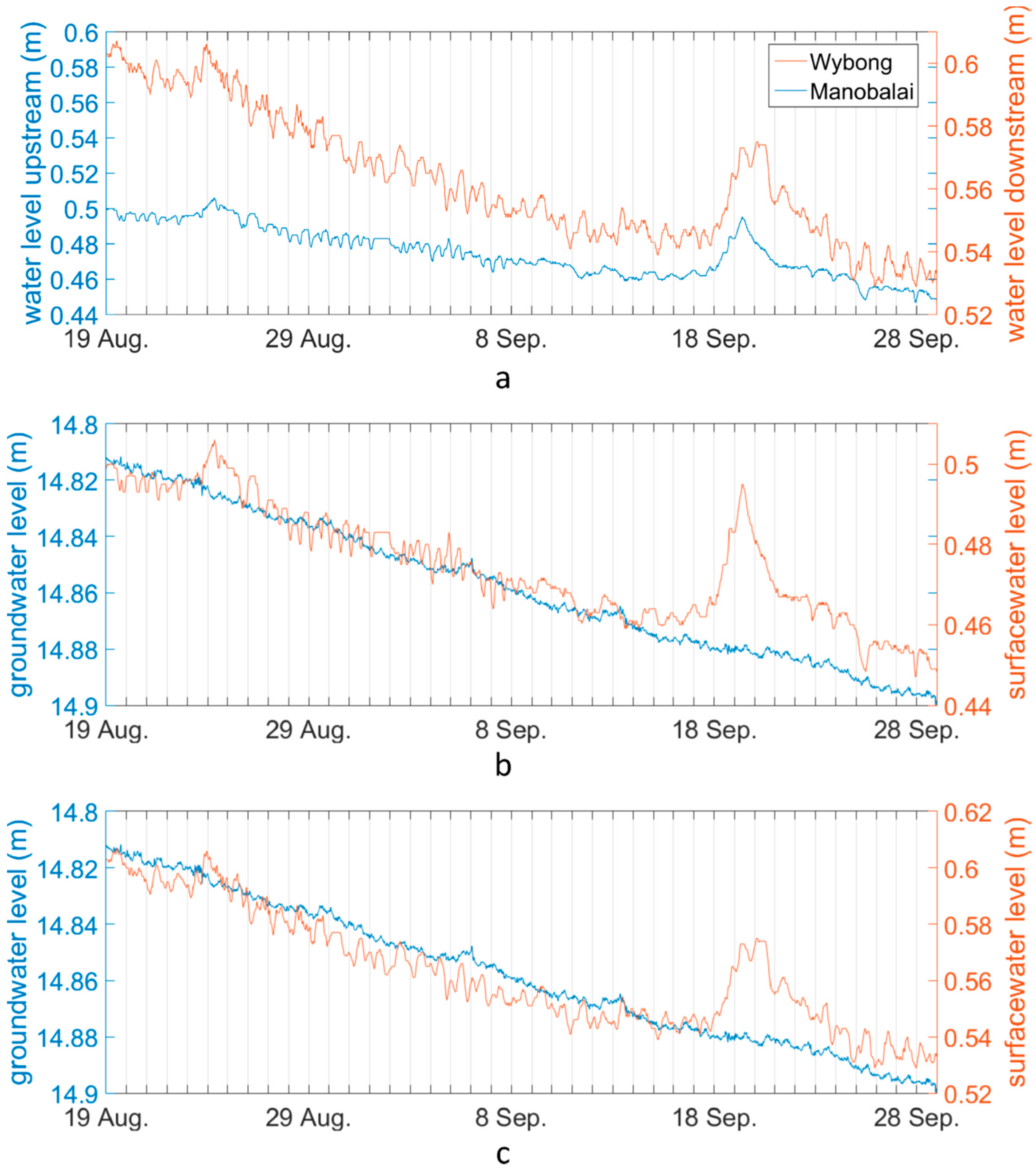
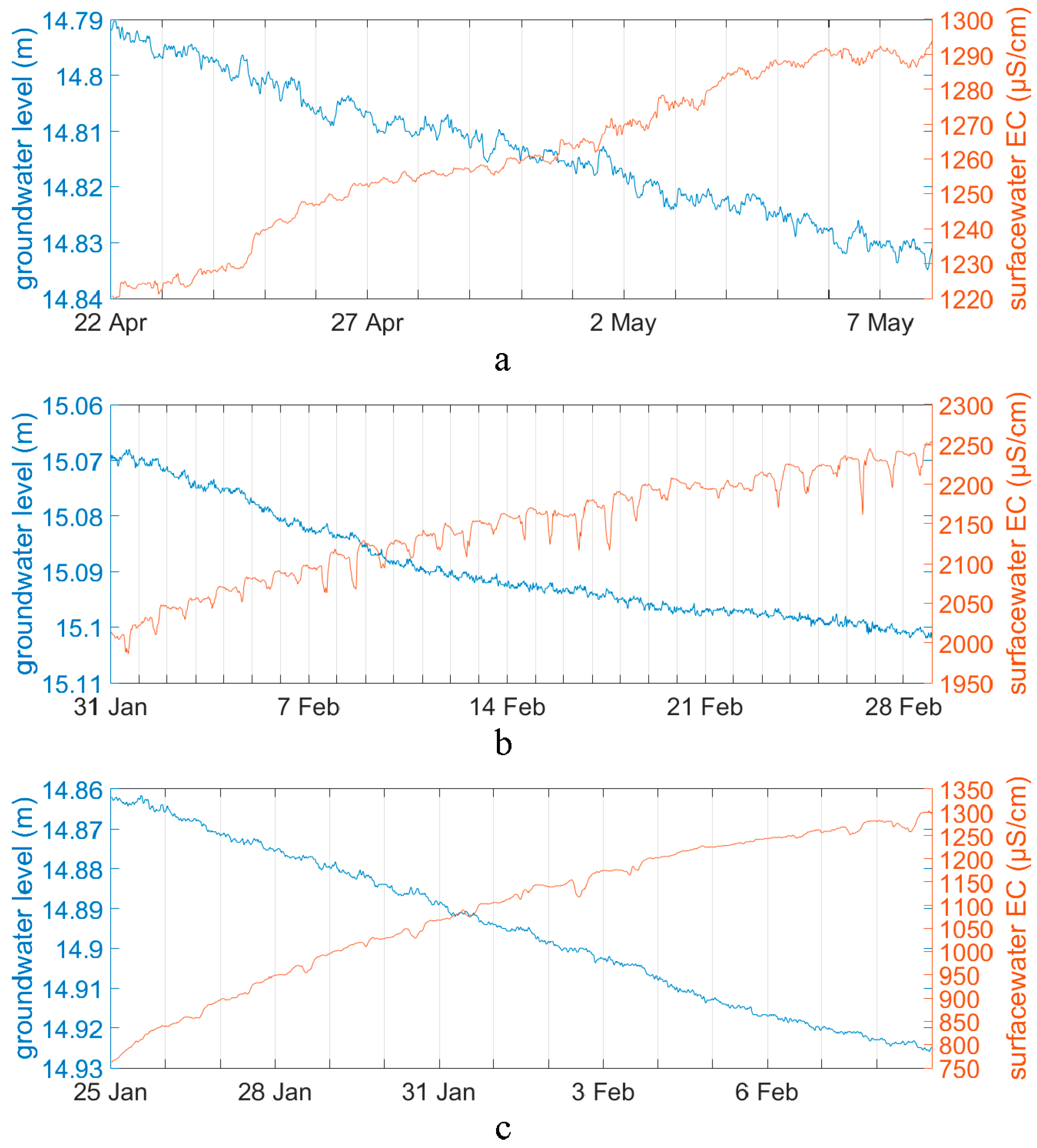
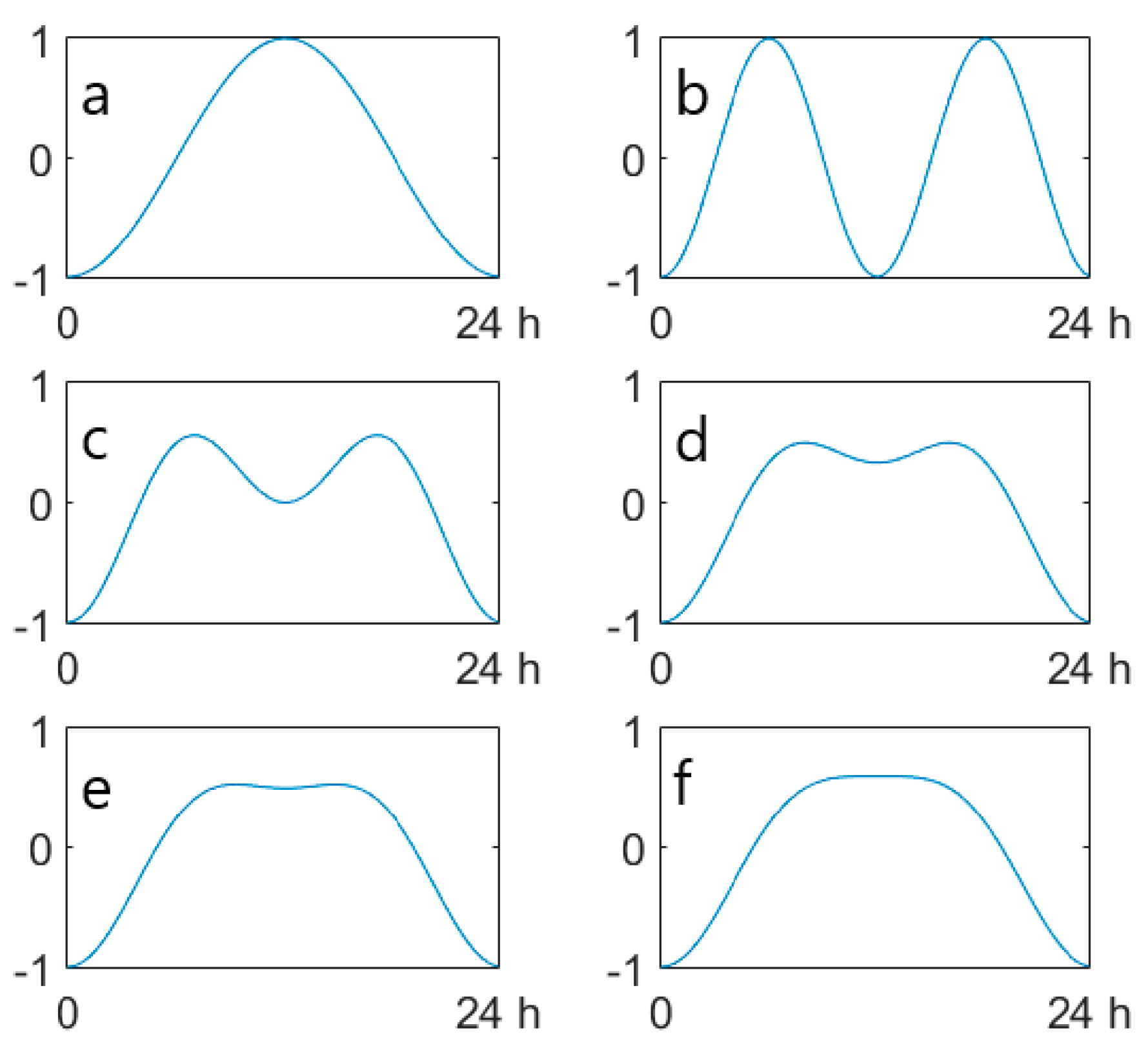
Semidiurnal oscillations in a streamwater level were also studied for another river, Wybong, in Australia/New South Wales—this river belongs to the Hunter River basin. The oscillations are similar to those found in groundwater level in the same catchment (with different phasing due to different positions of river gauges on river (separated by a 9.9-km straight line distance; see Figure 7). Figure 7 shows the similar semidiurnal variations in surface and ground waters. These similarities suggest a causal relationship between the river and groundwater not only at the super-daily scale but also at the semidiurnal scale. However, orthotidal signals in river level/discharge are rarely found; the proper parameter for this river is the specific conductivity (EC), as already stated by an incipient study [14] (samples in Figure 8). In Wybong River catchment, EC is measured on a periodic basis only at Wybong. This parameter rarely exhibits two clearly distinguishable peaks per day. This behavior is caused by the very strong diurnal cycle; when weaker semidiurnal cycles are added in a time series with strong diurnal cycles, diurnal cycles with special shapes are created depending on the amplitudes of the mixed signals (for S1+S2, see Figure 9; for S1+M2, see Briciu [17]).

No significant tidal oscillations in water level (gage height/discharge) at both stations in Alapaha River catchment or in the specific conductivity parameter (measured periodically only at Jennings) were found. This leads to the conclusion that the newly added parameter—water temperature (from 2016, with regular measurements done at high frequency, 96/day)—at both gages is sensitive to orthotides probably due to both local hydrogeological conditions and high precision of the instruments.

We detected 3 long time intervals with persistent orthotides of EC (25 °C) in 2013, 2014, and 2017, containing 117, 54, and 52 consecutive days, respectively (Supplementary Figures S8–S10). The wavelet transform indicates significant semidiurnal signals (Supplementary Figure S11), while WTC analyses of groundwater level and river EC show an evolution in antiphase of these parameters (Supplementary Figure S12; the antiphase is indicated by the arrows pointing left). As there is a similar antiphase relationship between atmospheric pressure and river EC (Supplementary Figure S13), the groundwater level and atmospheric pressure are in phase, suggesting that water from a confined aquifer discharges into the river and exports the groundwater tides. In the last decade, some researchers [29] found confined conditions close to topographic surfaces in other areas of the globe and suggested that this could lead to special exchanges between groundwater and rivers. In Wybong River catchment, a saline groundwater discharge is responsible for the orthotidal signal found in EC [14]. This groundwater flows in a confined aquifer composed of fractured sandstones and conglomerates (Narrabeen Group) [30].

FFT analyses indicate that S2 is present in Wybong River EC; this signal originates in groundwater as result of periodic changes in atmospheric pressure (Supplementary Figure S14). The T_TIDE analysis of the S2 and M2 tidal components indicate that S2 is indeed dominant even in groundwater (

Table 3. Details of the selected semidiurnal constituents, M2 and S2, found with T_TIDE in Wybong River catchment (tidal amplitude and phase with 95% CI estimates; phases at central time).

Time Interval	Site-Parameter	Tidal Component	Period (h)	Amplitude *	Amplitude Error *	Phase (°)	Phase Error (°)	Signal to Noise Ratio
24 July–17 November 2013	river specific conductivity	M2	12.42	1.5291	1.425	279.46	64.17	1.2
		S2	12	9.1281	1.346	239.58	8.78	46
	groundwater level	M2	12.42	0.0002	0	92.14	29.2	4.3
		S2	12	0.0007	0	66.24	10.74	45
14 August–6 October 2014	river specific conductivity	M2	12.42	1.0928	1.945	29.59	115.94	0.32
		S2	12	11.3425	2.61	233.4	10.78	19
	groundwater level	M2	12.42	0.0001	0	135.83	39.69	2.2
		S2	12	0.0005	0	59.38	7.37	74
15 April 15–5 June 2017	river specific conductivity	M2	12.42	0.6213	1.212	212.38	133.85	0.26
		S2	12	6.6299	1.673	241.32	12.59	16
	groundwater level	M2	12.42	0.0001	0	21.41	94.47	0.46
		S2	12	0.0006	0	53.51	18.41	12

* Units in µS/cm for streamwater and in m for groundwater.

). The highest amplitudes observed for the S2 and M2 signals in streamwater are 11.3 µS/cm and 1.5 µS/cm, respectively.

When M2 has an SNR > 1 in river EC, it is in antiphase with M2 in groundwater, similar to the relationship of S2 in both environments. By using the newer and longer time series in this study, we confirm the presence of orthotides in Wybong River, as previously stated by Jasonsmith et al. [14], but we highlight the greater importance of S2 over M2.

A perfect match of streamwater and groundwater oscillations, e.g., observing them in exact phase or antiphase, is hard to find. The lags between cause and effect were previously observed and discussed by specialists in the case of earth/atmospheric tides (causes) and groundwater tides (effect) [31]. The phase difference between tides in different environments are caused by the time needed for a signal to propagate in space. The phase difference between various semidiurnal oscillation drivers (e.g., earth and atmospheric tides) has an impact on the recorded groundwater periodic variation [32]. Also, in the case of groundwater tides, more alternative causes of phase shift were indicated, such as groundwater flow and aquifer characteristics (e.g., rock porosity, fracture planes, and the compressibility of the surrounding aquifers) [33,34,35,36]. The degree of an aquifer confinement and anisotropy impacts the propagation of tides [37]. Overall, the properties of the geologic strata are very important in the behavior of groundwater tides [38]. Methods to assess the influence of the local geology and environment on groundwater tide characteristics, such as phase shifts, range from analyzing special conditions [39] to applying various mathematical techniques. The decomposition of water-level time series containing tidal oscillations might be a useful tool for simplifying the data analysis [40]. The characteristics of the groundwaters in various aquifers are responsible for the delayed orthotidal signal found in rivers. The signal export into rivers may be produced continuously or not in space and time and at different intensities, which affect the chances of the signal to be detected, especially when other natural variations tend to overwrite the periodic changes of interest.

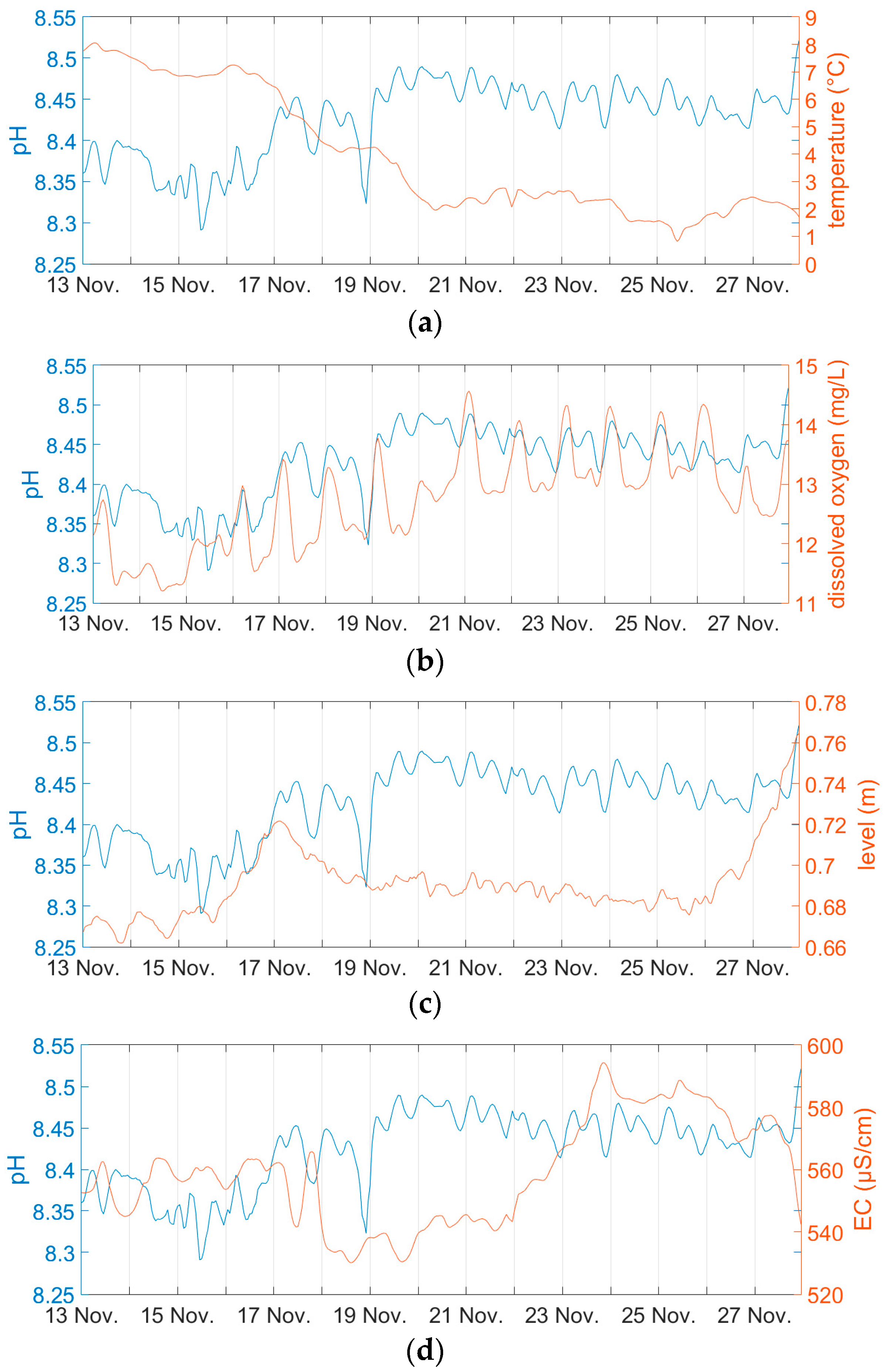
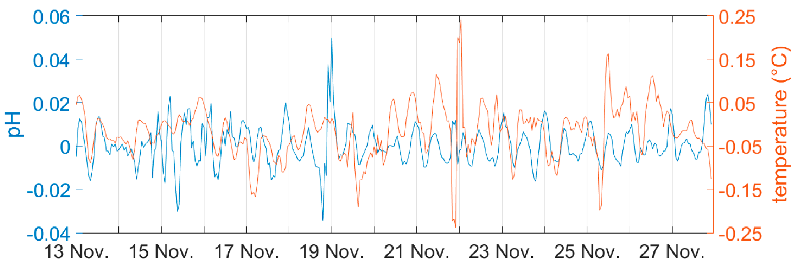
Semidiurnal variations in other parameters of streamwaters were found for Suceava River, especially for pH and dissolved oxygen time series (Figure 10). These oscillations seem to be related to similar oscillations in temperature and were recorded because of the rapid decrease in water temperature (~8 °C over a period of 15 days) caused by air temperature decrease. This temperature decrease led to an increased amplitude of the measured semidiurnal oscillations, probably due to the local groundwater discharging warmer water into river (Figure 11). Because of the interdependence of various water parameters, semidiurnal oscillations can be detected in the time series of many other parameters, other than the already consecrated level, specific conductivity, and temperature. This discovery pattern was previously observed in the case of the diurnal cycle of streamwaters.

4. Conclusions

Orthotides were detected in time series of Alapaha River water temperature. The tidal coefficients correlate with those in earth and atmospheric tides. S2 and M2 were detected as statistically significant signals in wavelet and T_TIDE analyses. For the first time, orthotides are described in relation to moon phases; also, unique time frame samples are displayed showing the similar evolution of gravitational acceleration and streamwater temperature. Orthotides in Wybong River indicate a stronger influence of atmospheric tides than earth tides, as revealed by the strong S2 signal.

The detection of the semidiurnal oscillations in multiple parameters indicates the important environmental impact of the small periodic natural changes. Quantifying the orthotides is useful for better understanding/decrypting of “noise” in water time series and for predictions of higher precision. Newer instruments in the field (with higher precision and recording more parameters) will slowly reveal more and more orthotidal rivers. Describing in detail the export of an orthotidal signal from groundwater into river is a task yet to be acquired. Probably, the next step is to successfully separate the thermal diurnal cycle from the tidal diurnal cycles in some ideal time series and to find new methods from the classical tidal potamology.

References

- Hoitink, A.J.F.; Jay, D.A. Tidal river dynamics: Implications for deltas. Rev. Geophys. 2016, 54, 240–272. [Google Scholar] [CrossRef]
- Dai, Z.; Du, J.; Tang, Z.; Ou, S.; Brody, S.; Mei, X.; Jing, J.; Yu, S. Detection of linkage between solar and lunar cycles and runoff of the world’s large rivers. Earth Space Sci. 2019, 6, 914–930. [Google Scholar] [CrossRef]
- Troxell, H.C. The diurnal fluctuation in the ground-water and flow of the Santa Anna River and its meaning. Trans. AGU 1936, 17, 496–504. [Google Scholar] [CrossRef]
- Briciu, A.-E.; Oprea-Gancevici, D.I. Diurnal thermal profiles of selected rivers in Romania. SGEM2015 Conf. Proc. 2015, 1, 221–228. [Google Scholar]
- Nimick, D.A.; Gammons, C.H.; Parker, S.R. Diel biogeochemical processes and their effect on the aqueous chemistry of streams: A review. Chem. Geol. 2011, 283, 3–17. [Google Scholar] [CrossRef]
- Gribovszki, Z.; Szilagyi, J.; Kalicz, P. Diurnal fluctuations in shallow groundwater levels and streamflow rates and their inter-pretation—A review. J. Hydrol. 2010, 385, 371–383. [Google Scholar] [CrossRef]
- Robinson, T.W. Earth tides shown by fluctuations of water levels in wells in New Mexico and Iowa. Trans. AGU 1939, 20, 656–666. [Google Scholar] [CrossRef]
- Lambert, W.D. Report on earth tides. U.S. Coast Geodet. Surv. 1940, 223, 1–24. [Google Scholar]
- Bredehoeft, J.D. Response of well-aquifer systems to earth tides. J. Geophys. Res. 1967, 72, 3075–3087. [Google Scholar] [CrossRef]
- Merritt, M.L. Estimating hydraulic properties of the Floridan aquifer system by analysis of earth-tide, ocean-tide, and barometric effects, Collier and Hendry Counties, Florida. U.S. Geol. Surv. Water Resour. 2004, 2003–4267. [Google Scholar] [CrossRef]
- Luque-Espinar, J.A.; Pardo-Igúzquiza, E.; González-Ramón, A.; López-Chicano, M.; Durán-Valsero, J.J.; Pulido-Velázquez, D. Spectral Analysis of Time Series of Carbonate Aquifer of Sierra Gorda. In Advances in Karst Science; Renard, P., Bertrand, C., Eds.; Springer: Berlin/Heidelberg, Germany, 2017. [Google Scholar]
- Barberio, M.D.; Gori, F.; Barbieri, M.; Billi, A.; Devoti, R.; Doglioni, C.; Petitta, M.; Riguzzi, F.; Rusi, S. Diurnal and semidiurnal cyclicity of Radon (222Rn) in groundwater, Giardino Spring, Central Apennines, Italy. Water 2018, 10, 1276. [Google Scholar] [CrossRef]
- Briciu, A.-E. Wavelet analysis of lunar semidiurnal tidal influence on selected inland rivers across the globe. Sci. Rep. 2014, 4, 4193. [Google Scholar] [CrossRef] [PubMed]
- Jasonsmith, J.F.; Macdonald, B.C.T.; White, I. Earth-tide-induced fluctuations in the salinity of an inland river, New South Wales, Australia: A short-term study. Environ. Monit. Assess. 2017, 189, 188. [Google Scholar] [CrossRef] [PubMed]
- Kulessa, B.; Hubbard, B.; Brown, G.H.; Becker, J. Earth tide forcing of glacier drainage. Geophys. Res. Lett. 2003, 30, 1011. [Google Scholar] [CrossRef]
- Briciu, A.-E.; Mihăilă, D.; Oprea, D.I.; Bistricean, P.-I.; Lazurca, L.G. Orthotidal signal in the electrical conductivity of an inland river. Environ. Monit. Assess. 2018, 190, 282. [Google Scholar] [CrossRef]
- Briciu, A.-E. Diurnal, semidiurnal, and fortnightly tidal components in orthotidal proglacial rivers. Environ. Monit. Assess. 2018, 190, 160. [Google Scholar] [CrossRef]
- Cerveny, R.S.; Svoma, B.M.; Vose, R.S. Lunar tidal influence on inland river streamflow across the conterminous United States. Geophys. Res. Lett. 2010, 37, L22406. [Google Scholar] [CrossRef]
- Torrence, C.; Compo, G.P. A practical guide to wavelet analysis. Bull. Am. Meteor. Soc. 1998, 79, 61–78. [Google Scholar] [CrossRef]
- Ng, E.K.W.; Chan, J.C.L. Geophysical applications of partial wavelet coherence and multiple wavelet coherence. J. Atmos. Oceanic Technol. 2012, 29, 1845–1853. [Google Scholar] [CrossRef]
- Grinsted, A.; Moore, J.C.; Jevrejeva, S. Application of the cross wavelet transform and wavelet coherence to geophysical time series. Nonlin. Process. Geophys. 2004, 11, 561–566. [Google Scholar] [CrossRef]
- Torrence, C.; Webster, P. Interdecadal Changes in the ENSO-Monsoon System. J. Clim. 1999, 12, 2679–2690. [Google Scholar] [CrossRef]
- Pawlowicz, R.; Beardsley, B.; Lentz, S. Classical tidal har-monic analysis including error estimates in MATLAB using T_TIDE. Comput. Geosci. 2002, 28, 929–937. [Google Scholar] [CrossRef]
- Tamura, Y. A harmonic development of the tide generating potential. Bull. Info. Marées Terr. 1987, 99, 6813–6855. [Google Scholar]
- Dehant, V.; Defraigne, P.; Wahr, J. Tides for a convective Earth. J. Geophys. Res. 1999, 104, 1035–1058. [Google Scholar] [CrossRef]
- Miller, J.A. Groundwater atlas of the United States: Segment 6, Alabama, Florida, Georgia, and South Carolina. U.S. Geol. Surv. Hydrol. Investig. Atlas 1993, 30, 116. [Google Scholar]
- Plummer, L.N.; Busenberg, E.; Drenkard, S.; Schlosser, P.; Ekwurzel, B.; Weppernig, R.; McConnell, J.B.; Michel, R.L. Flow of river water into a karstic limestone aquifer—2. Dating the young fraction in groundwater mixtures in the Upper Floridan aquifer near Valdosta, Georgia. Appl. Geochem. 1998, 13, 1017–1043. [Google Scholar] [CrossRef]
- Planert, M. Simulation of Regional Ground-Water Flow in the Suwannee River Basin, Northern Florida and Southern Georgia. U.S. Geol. Surv. Sci. Investig. Rep. 2007, 2007–5031. [Google Scholar] [CrossRef]
- Acworth, R.I.; Brain, T. Calculation of barometric efficiency in shallow piezometers using water levels, atmospheric and earth tide data. Hydrogeol. J. 2008, 16, 1469–1481. [Google Scholar] [CrossRef]
- Jasonsmith, J.F. Origins of Salinity and Salinisation Processes in the Wybong Creek Catchment, New South Wales, Australia. Ph.D. Thesis, Australian National University, Canberra, Australia, 2010. [Google Scholar]
- Hsieh, P.A.; Bredehoeft, J.D.; Farr, J.M. Determination of aquifer transmissivity from Earth tide analysis. Water Resour. Res. 1987, 23, 1824–1832. [Google Scholar] [CrossRef]
- Acworth, R.I.; Halloran, L.J.S.; Rau, G.C.; Cuthbert, M.O.; Bernardi, T.L. An objective frequency domain method for quantifying confined aquifer compressible storage using Earth and atmospheric tides. Geophys. Res. Let. 2016, 43, 11671–11678. [Google Scholar] [CrossRef]
- Hanson, J.M.; Owen, L.B. Fracture orientation analysis by the solid earth tidal strain method. In Proceedings of the 57th Annual Fall Technical Conference and Exhibition of the Society of Petroleum Engineers of AIME, American Institute of Mechanical Engineers, New Orleans, LA, USA, 26–29 September 1982. [Google Scholar]
- Bower, D.R. Bedrock fracture parameters from the interpretation of well tides. J. Geophys. Res. 1983, 88, 5025–5035. [Google Scholar] [CrossRef]
- Gieske, A.; De Vries, J.J. An analysis of earth-tide-induced groundwater flow in eastern Botswana. J. Hydrol. 1985, 82, 211–232. [Google Scholar] [CrossRef]
- McMillan, T.C.; Rau, G.C.; Timms, W.A.; Andersen, M.S. Utilizing the impact of earth and atmospheric tides on groundwater systems: A review reveals the future potential. Rev. Geophys. 2019, 57, 281–315. [Google Scholar] [CrossRef]
- Shuai, P.; Knappett, P.S.K.; Hossain, S.; Hosain, A.; Rhodes, K.; Ahmed, K.M.; Cardenas, M.B. The impact of the degree of aquifer confinement and anisotropy on tidal pulse propagation. Ground Water 2017, 55, 519–531. [Google Scholar] [CrossRef] [PubMed]
- Rojstaczer, S.; Agnew, D.C. The influence of formation material properties on the response of water levels in wells to Earth tides and atmospheric loading. J. Geophys. Resear. 1989, 94, 12403–12411. [Google Scholar] [CrossRef]
- Zhang, H.; Shi, Z.; Wang, G.; Sun, X.; Yan, R.; Liu, C. Large earthquake reshapes the groundwater flow system: Insight from the water-level response to earth tides and atmospheric pressure in a deep well. Water Resour. Res. 2019, 55, 4207–4219. [Google Scholar] [CrossRef] [Green Version]
- Lee, M.; You, Y.; Kim, S.; Kim, K.T.; Kim, H.S. Decomposition of water level time series of a tidal river into tide, wave and rainfall-runoff components. Water 2018, 10, 1568. [Google Scholar] [CrossRef] [Green Version]
Figure 1.
Semidiurnal oscillations found in Alapaha River during 2–24 October 2017. Comparison of river water temperature at Statenville and groundwater level (depth to water) at Valdosta: (a) raw data; (b) smoothed differences between adjacent values; (c) values detrended though additive decomposition; and (d) scalogram of the wavelet transform of streamwater temperature (as differences between adjacent values).
Figure 2.
Fast Fourier Transform (FFT) analyses of time series in the Valdosta–Statenville area for time intervals in 2017 and 2018: Diurnal and semidiurnal signals were found during (a) 6 September–11 November 2018 and (b) 6 December 2017–2 February 2018 in (1) streamwater temperature, (2) groundwater level, and (3) atmospheric pressure.
Figure 3.
Causal relationship between atmospheric pressure and groundwater level at Valdosta—an example of the representative antiphase is shown here for 2–24 October 2017 (displayed data is the difference between adjacent values, smoothed by a moving average filter with a span of 11 values (1 day = 96 values)).
Figure 4.
Orthotidal oscillations in streamwater temperature were found simultaneously in 2 monitoring points of Alapaha River (Statenville and Jennings)—orthotides were found in the nontidal reach of Alapaha River during (a) 3 August–1 September 2017; (b) 2 October–24 October 2017; (c) 6 December 2017–2 February 2018; and (d) 6 September–11 November 2018.
Figure 5.
Similar evolution of earth tides and semidiurnal cycles in Alapaha River water temperature during some fortnightly (15 days) time intervals in 2017: The smoothed differences between adjacent values of streamwater temperature are compared to the variations of (a) gravity and (b) atmospheric pressure during 17–31 August 2017; the same for 10–25 October 2017 (c,d)—the arrows indicate the unpaired peaks; the atmospheric pressure (smoothed differences) does not explain the unpaired peaks that are also found in groundwater level (smoothed differences).
Figure 6.
Causal relationship between earth tides and semidiurnal cycles in Alapaha River water temperature during two fortnightly time intervals: the smoothed differences between adjacent values of streamwater temperature are compared to the variations of gravity during (a) 18 October–1 November 2016 and (b) 11–25 October 2018. The arrows indicate the unpaired peaks in streamwater temperature.
Figure 7.
Orthotides in Wybong River catchment were found in both groundwater and streamwater level oscillations. Similar oscillations were found simultaneously in two monitoring points (a), and the upstream (Manobalai) (b) and downstream (Wybong) (c) streamwater levels have similarities with the groundwater level measured at Wybong (smoothed data; 19 August–28 September 2012).
Figure 8.
The specific conductivity of Wybong River is a better recorder of orthotides. The evolution of streamwater specific conductivity (EC) at Wybong versus groundwater level (smoothed data) indicates antiphases at the sub-daily and super-daily scales (with diurnal and semidiurnal oscillations included): (a) 22 April –7 May 2013; (b) 31 January–28 February 2015; and (c) 25 January–8 February 2016.
Figure 9.
The addition of sine waves of different wavelengths and amplitudes indicates how apparently irregular diurnal peaks are hiding other cycles. This is the case for the theoretical evolution of a diurnal cycle composed of an S1 sine wave and an S2 sine wave with identical moments of the minima values: (a) S1; (b) S2; (c) (S1 + S2)/2; (d) (2S1 + S2)/3; (e) (3S1 + S2)/4; and (f) (4S1 + S2)/5.
Figure 10.
Semidiurnal variations were observed in Suceava River in the time series of many parameters, especially the pH—signals with various amplitudes that might be caused by variations of groundwater input into the river and are similar to those observed in the evolution of pH were found in (smoothed data; 13–27 November 2018) (a) temperature; (b) dissolved oxygen; (c) water level; and (d) specific conductivity (25 °C).
Figure 11.
The synchronous evolution of semidiurnal cycles of Suceava River pH and temperature is not an effect of the standard inverse relationship that is usually observed between these parameters. Changes in water parameters were observed due to the strong temperature decrease over a fortnightly period (13–27 November 2018; plotted data represent smoothed difference between adjacent values).