Numerical Simulations of Non-Breaking, Breaking and Broken Wave Interaction with Emerged Vegetation Using Navier-Stokes Equations


School of Civil Engineering and Transportation, South China University of Technology, Guangzhou 510640, China
*
Author to whom correspondence should be addressed.
Water 2019, 11(12), 2561; https://doi.org/10.3390/w11122561
Submission received: 22 October 2019
/
Revised: 27 November 2019
/
Accepted: 3 December 2019
/
Published: 4 December 2019
(This article belongs to the Special Issue Modeling and Numerical Simulation of Ocean and Coastal Waves)
Abstract
:Coastal plants can significantly dissipate water wave energy and services as a part of shoreline protection. Using plants as a natural buffer from wave impacts remains an attractive possibility. In this paper, we present a numerical investigation on the effects of the emerged vegetation on non-breaking, breaking and broken wave propagation through vegetation over flat and sloping beds using the Reynolds-average Navier-Stokes (RANS) equations coupled with a volume of fluid (VOF) surface capturing method. The multiphase two-equation k-ω SST turbulence model is adopted to simulate wave breaking and takes into account the effects enhanced by vegetation. The numerical model is validated with existing data from several laboratory experiments. The sensitivities of wave height evolution due to wave conditions and vegetation characteristics with variable bathymetry have been investigated. The results show good agreement with measured data. For non-breaking waves, the wave reflection due to the vegetation can increase wave height in front of the vegetation. For breaking waves, it is shown that the wave breaking behavior can be different when the vegetation is in the surf zone. The wave breaking point is slightly earlier and the wave height at the breaking point is smaller with the vegetation. For broken waves, the vegetation has little effect on the wave height before the breaking point. Meanwhile, the inertia force is important within denser vegetation and is intended to decrease the wave damping of the vegetation. Overall, the present model has good performance in simulating non-breaking, breaking and broken wave interaction with the emerged vegetation and can achieve a better understanding of wave propagation over the emerged vegetation.
1. Introduction
The vegetation patches are proven to be effective in surface wave attenuation, which plays an important role in coastal defense by reducing incoming wave energy, stabilizing shore sediments and improving water quality. Wave transmission and attenuation characteristics are important in determining the location and amount of plants required for shore protection applications [1]. The vegetation can significantly alter mean flows, velocity profiles and generate additional turbulence production [2,3,4]. Harada et al. [2] demonstrate that the vegetation is as effective as concrete breakwater structures for holding back the sea waves and minimizing wave forces. Actually, due to the increase of coastal flooding and the rising sea-level, the efficiency of vegetation to reduce the wave energy has been generally recognized. Numerous studies have focused on this topic [5,6,7,8,9,10].
For laboratory experiments, most of them are using artificial vegetation, including rigid stems and flexible strips to mimic the real vegetation. Dalrymple et al. [5] considered the vegetation as the vertical cylinders of small diameter. The wave energy loss attributed to the fluid motion was estimated. Arnaud et al. [11] showed that there exists an oscillating behavior of the reflection coefficient in the direction of wave propagation. As the wave period increases, the oscillation decreases. On the other hand, the flexibility of the vegetation also has a strong influence on wave behavior. In general, greater flexibility results in more vegetation deformation under fluid motion and limits wave dissipation [12,13]. Luca et al. [14] carried out experiments for dense meadow, where the flexibility of the blade became a dominant factor. They concluded that the flexibility has considerably weakened the wave attenuation attributable to the vegetation in the meadow. Mendez et al. [6] conducted experiments on vegetation fields over varying bathymetry. A wave damping formulation for slope bottom conditions and breaking waves was presented. Maza et al. [15] also studied the hydrodynamics of the emerged vegetation for solitary waves. It was concluded that the macroscopic approach was able to produce satisfactory results if proper drag coefficient was obtained. Strusinska-Correia et al. [16] studied the influence of vegetation parameterization on wave height evolution and the bore propagation processes together with the hydraulic vegetation resistance subjected to tsunami-like solitary waves and tsunami bores.
In the field, the vegetation is far more complicated and may differ primarily in the species [17,18,19]. Knutson et al. [17] conducted a field study to quantify wave attenuation in the grass marshes. The interaction of vegetation and waves is complex due to the variety of physical and biological conditions. The empirical drag coefficient could be species-dependent. Paul et al. [18] found that the higher the wave period is, the lower is the required density to initiate wave attenuation. Vanegas et al. [19] evaluated wave dissipation by conducting field data from Rhizophora patch in relation to the sea state. The drag coefficient used to calculate wave dissipation is variable over time depending on significant wave height and wave period.
With the developments of wave-vegetation theory, numerical models are also used to quantify wave attenuation due to the vegetation. The vegetation-induced wave dissipation can be modeled by either phase-average models, such as SWAN [20], mild slope equation [21] or phase-resolved models, such as Boussinesq-type equations [22], non-hydrostatic model [23] and Reynolds-average Navier-Stokes (RANS) equations for multiphase flows using the volume of fluid (VOF) method [24,25]. In their studies, the SWAN model and Boussinesq-type use a bottom friction term to account for the presence of vegetation. The non-hydrostatic model and the RANS equations, on the other hand, consider the vegetation flow by incorporating drag and inertia force terms. It is clear that the most common approach to model vegetation dissipated by the wave energy is including additional source terms in the conservation equations.
The previous studies have investigated the dynamics of turbulence generated during wave breaking and the interaction with the vegetation [26,27,28,29]. Their results show that the turbulence should be taken into account for better prediction of mean flow and wave height. Full Navier-Stokes models make it possible to include turbulence effects. Brown et al. [28] compared several two equation turbulence closure models for spilling and plunging breakers. They found that if a RANS turbulence was applied, the number of iterations was reduced. Therefore, the computational time decreased, compared to assume no turbulence. The representation of turbulence by large-eddy simulations (LES) was also investigated by Lubin et al. [30,31]. The wave overturning and air entrainment are discussed using the LES method. The wave-height evolution can be predicted well if the subgrid model is implemented appropriately and the mesh is fine enough to resolve the filtered velocity field. Another factor that contributes to the turbulence is the interaction with vegetation. Hiraoka et al. [3] showed that the existence of vegetation enhances the turbulence and proposed a new turbulence model, which was also adopted by other researchers [4,24].
However, the studies about the hydrodynamics of breaking waves on the emerged vegetation are limited. The effect of emerged vegetation controlling wave breaking is not fully understood. For example, the general agreements are that wave attenuation increased with the vegetation width and density, but no clear relationship to wave breaking behavior (e.g., breaking point and breaking wave height). Although there are recent studies [16,20,32] examining the capability of numerical models to resolve the interaction of breaking waves and the vegetation, the studies of the fully Navier-Stokes models including turbulence effects are generally scarce. Therefore, the performance of RANS models to simulate the interaction of the breaking waves with the vegetation is still not clear and worthy of further investigation.
The main goal of this work is to provide a practical numerical model for nonbreaking, breaking and broken waves on the emerged vegetation. The governing equations are based on RANS equations with open-source toolbox OpenFOAM. The momentum equations incorporate drag and inertia force terms for the interaction between the waves and the vegetation. The VOF method is utilized to capture the free surface. To investigate wave propagation including wave breaking, a multiphase k-ω SST turbulence model with the effects of the vegetation is adopted for simulation. The paper is organized as follows. The numerical model is described in Section 2, including boundary conditions and discretization description. Comparisons between the experimental and numerical results and discussions are discussed in Section 3. The conclusions obtained in the present study are provided in Section 4.
2. Methodology
2.1. Governing Equations
The numerical model is modeled in OpenFOAM by RANS equations, which consist of a mass conservation equation and a momentum equation for incompressible viscous flows. The free surface is captured with the VOF method, written as the following form:
where is the time, (1, 2, 3; ) are the coordinates of a Cartesian frame. are the Cartesian components of the fluid velocity, is the acceleration of gravity, is the surface tension coefficient, is the mean curvature of the interface, is the molecular dynamic viscosity and is the turbulent dynamic viscosity, is the pressure in excess of the hydrostatic. is the resistance force induced by the vegetation. is the volume fraction of fluid using the VOF approach. are artificial compressive velocity in order to compress the interface and are only active in the thin interface region. The density is calculated as .
The existence of the vegetation can be taken into account by incorporating the drag and inertia forces based on Morison’s formulation in the momentum equations [33]. The average force per unit volume within the vegetation zone is given by:
The first term on the right sides is drag forces and the second term is inertia forces. is the bulk drag coefficient. is the added-mass coefficient and set to a constant value, [34], is the stem diameter of the plant and is the amount of the vegetation per square meter.
2.2. Turbulence Model
The turbulence model is needed to simulate the wave-vegetation interaction including wave breaking. Several two-equation models (e.g., -; RNG -; -SST) are ranked according to their performance in simulation by Brown et al. [28]. It is clear that the rate of turbulence dissipation can become singular near the wall in the - and RNG - models, which could cause stability issues when simulating wave breaking. Here, more robust formulation, the - SST model, is chosen to appropriately calculate the Reynold stress due to its advantage of an accurate near-wall treatment and lower sensitivity to the free stream value of compared to - model. However, the standard - SST model proposed by Menter [35] can overestimate turbulence levels when simulating surface waves, which causes excessive wave damping during wave propagations, as shown by Devolder et al. [29]. Therefore, we adopt the multiphase - SST model to appropriately calculate the Reynolds stress, the turbulence kinetic energy and the specific dissipation rate are expressed from the following transport equations:
where is the production term of and is obtained as , is the turbulent dynamic viscosity, the last terms in Equation (6) and Equation (7) are source terms due to the vegetation resistance. is the mean rate of strain of the flow. The empirical constants , and . and are blending functions, which is written as , is in the near-wall region and zero away from wall. β and γ are blended using Equation (8). and . Default values for and used in equation to calculate are , , , , , .
2.3. Boundary Conditions
In the inlet boundary, the velocity field and the location of the free surface were determined based on wave conditions in the experimental study according to the Stokes wave theory and the pressure was set to a gradient value such that the flux is specified by the wave velocity. The outlet used an active absorbing boundary. The atmosphere boundary was set to a mixed Dirichlet-Neumann condition for the velocity, pressure and volume fraction. The bottom boundary was set to a non-slip wall condition.
2.4. Numerical Methods
The numerical model is solved via the finite volume method. The pressure and velocity are calculated by the PIMPLE algorithm, which is a mixture between the splitting of operator (PISO) method and semi-implicit method for pressure-linked equations (SIMPLE) algorithms. The discretization schemes for the turbulence kinetic energy and specific dissipation rate are implemented using a Gauss upwind scheme. The time term is discretized by backward Euler time scheme, the convection term is discretized by the Gauss linear corrected scheme which has higher order than Gauss upwind to minimize numerical diffusion.
3. Results
3.1. Solitary Wave Propagation over the Slope
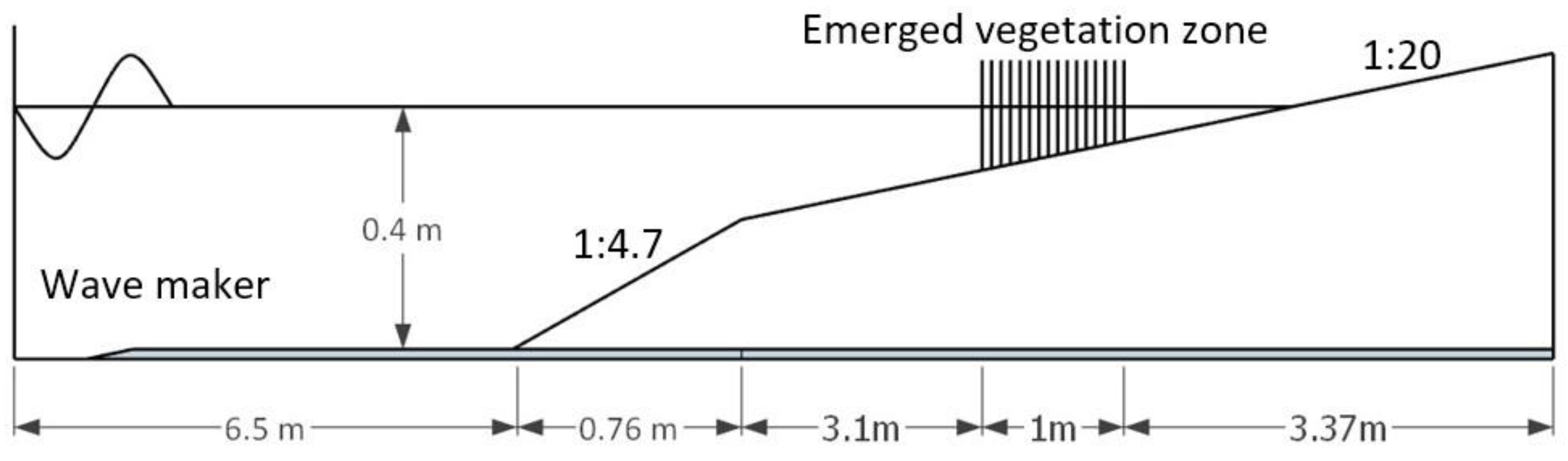
The numerical model is first validated by comparison with the experimental results for solitary wave propagation on the slope with the wooden cylinders conducted by Iimura et al. [8]. The experiments were conducted in a 15 m long, 0.4 m wide with two slopes, 1:4.7 and 1:20.5, as shown in Figure 1. The wooden cylinders were fixed on the slope with uniform and nonuniform density. The stems were always emerged and had a diameter of 0.005 m set in a staggered arrangement. The stem densities were N = 462, 1283 and 11,547 unit/m2 in case 1 to case 3, respectively. In case 4 and case 5, a combination of two stem densities, N = 722 and 2887 unit/m2 was used. The length of the stem ranged from 0.04 m to 1.0 m. The water depth was 0.4 m. The experimental conditions used by the present model are given in Table 1.
The grid size for numerical simulation is Δx = Δz = 0.01 m. Then, the zone close to free surface (between levels z = 0.35 m and 0.45 m) and slop is refined once in z direction, ending up in 0.005 m of vertical resolution. The final mesh has 68,494 cells. The simulation was parallelized into 12 processors (3.2 Ghz). The computational time was about 30 min for 30 s simulation. The vegetation-induced forces in the numerical model are determined by drag coefficient and the fluid velocity. Therefore, the drag coefficient is calibrated by comparing the calculated forces in the numerical results and the measured forces in the experiments. The drag coefficients listed in Table 1 are calibrated by the experimental results and are not constant for non-uniform arrangement vegetation in case 4 and case 5.
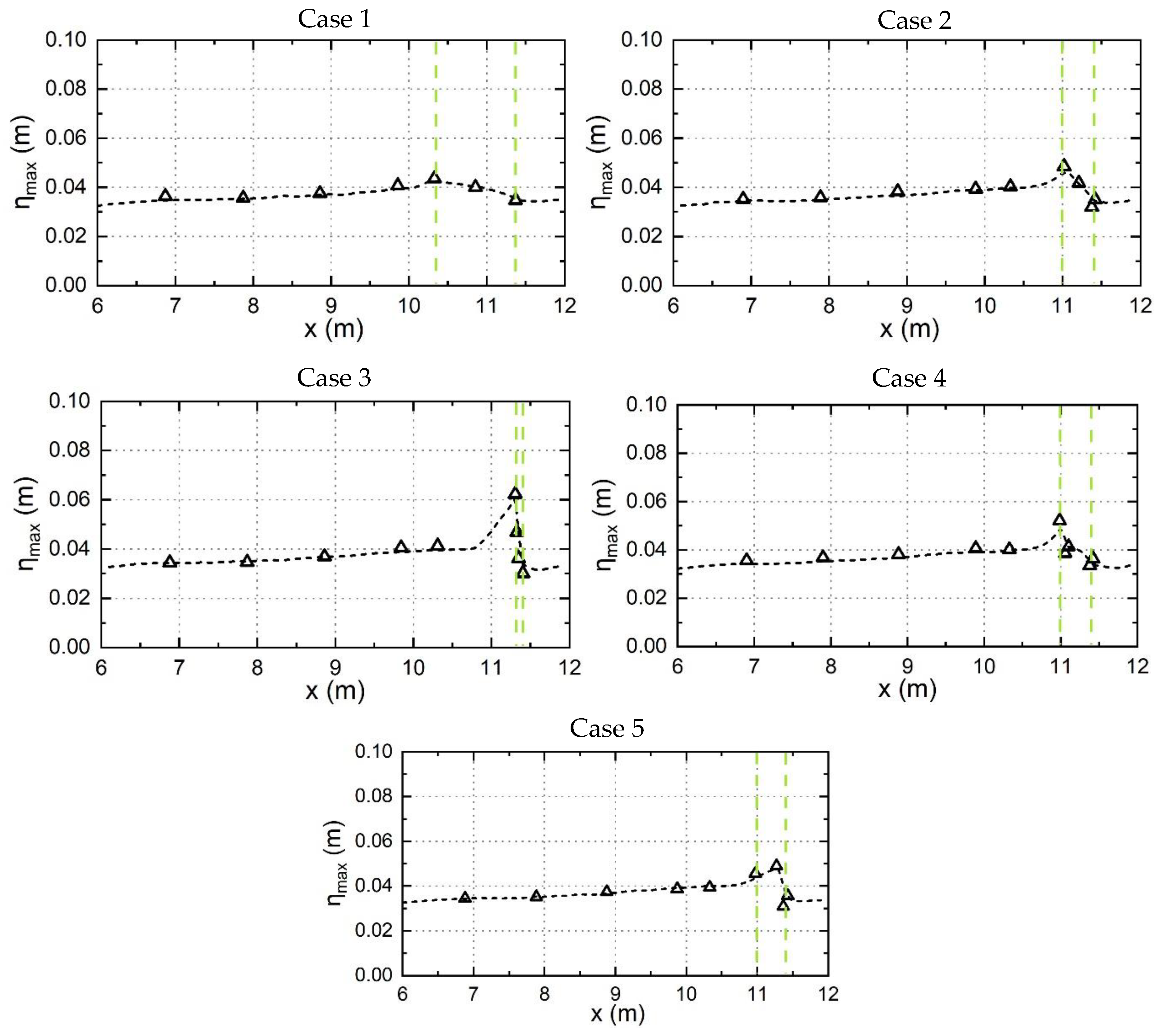
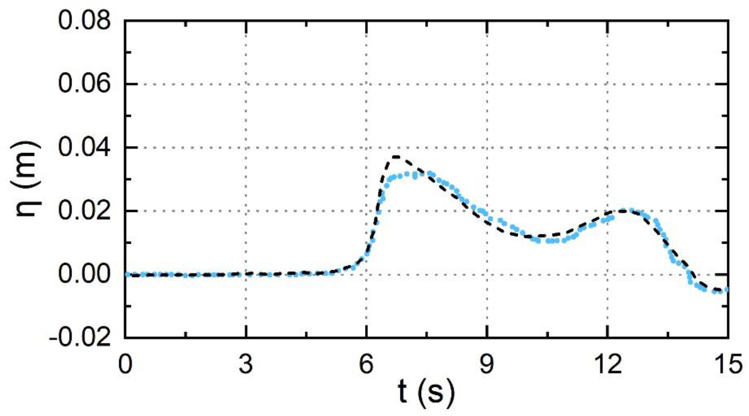
The calculated maximum free surface with the vegetation is shown in Figure 2. In general, the prediction of the maximum free surface in the present model shows good agreement with the experiments. The maximum free surface in front of the vegetation increases with increasing density of the vegetation, which is due to higher wave reflection. A comparison of the measured and calculated free surface time series at the end of the vegetation (x = 11.36 m) is shown in Figure 3 for case 3. The numerical results reproduce with high accuracy of the free surface, compared with the experiments. The difference observed between laboratory and numerical results is at the wave crest, which slightly overpredicts the peak of free surface.
3.2. Regular Wave Propagation over the Slope
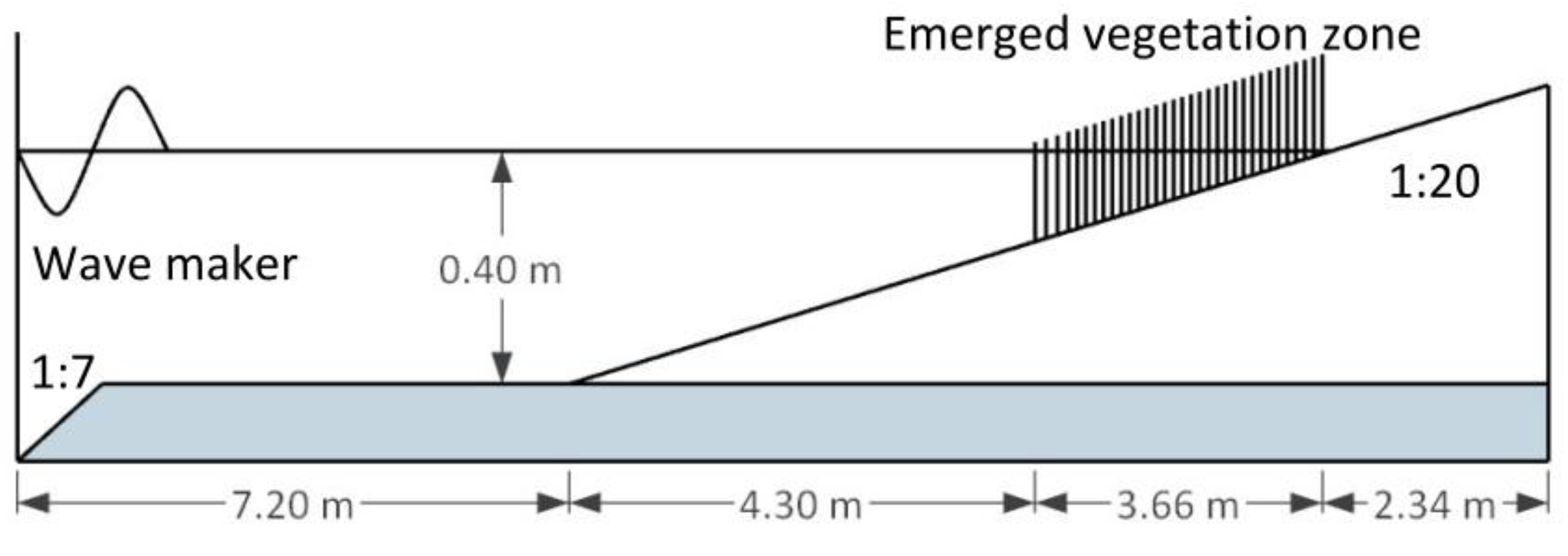
The experiments conducted at USDA-ARS National Sedimentation Laboratory in Oxford, Mississippi, USA by Wu et al. [36] were used to test the model against non-breaking and breaking wave interaction with vegetation over the slope as shown in Figure 4. The slope was m = 1:20. The vegetation was placed on the slope and was modeled by 0.2 m tall birch dowels with diameter of 3.2 mm in a staggered arrangement. The vegetation density was 3182 unit/m2 and the width of the vegetation was 3.7 m. The water depth was 0.4 m at the flatbed. The drag coefficient was calibrated as the bulk constant of 1.7 by comparing the wave heights, , of the measured data and the numerical results. According to Reeve et al. [34], the second-order Stokes wave theory was chosen here for wave generation. The experimental conditions used by the present model are given in Table 2.
The computational domain is 17.5 m long with the uniform grid discretization, having a grid size equal to 0.04 m in the horizontal direction and half of this value 0.02 m in the vertical one. Then, the zone close to the free surface (between levels z = 0.6 m and 0.8 m) and slop are refined twice in both x- and z-direction, ending up in 0.01 m of x direction and 0.005 m in the vertical one. The computational domain consists of 249,068 cells. The simulation was parallelized into 12 processors (3.2 Ghz). The computational time was about 70 min for 60 s simulation. To verify the simulated wave heights against the experiments, a series of wave gauges are set up for the measurements of the free surface.
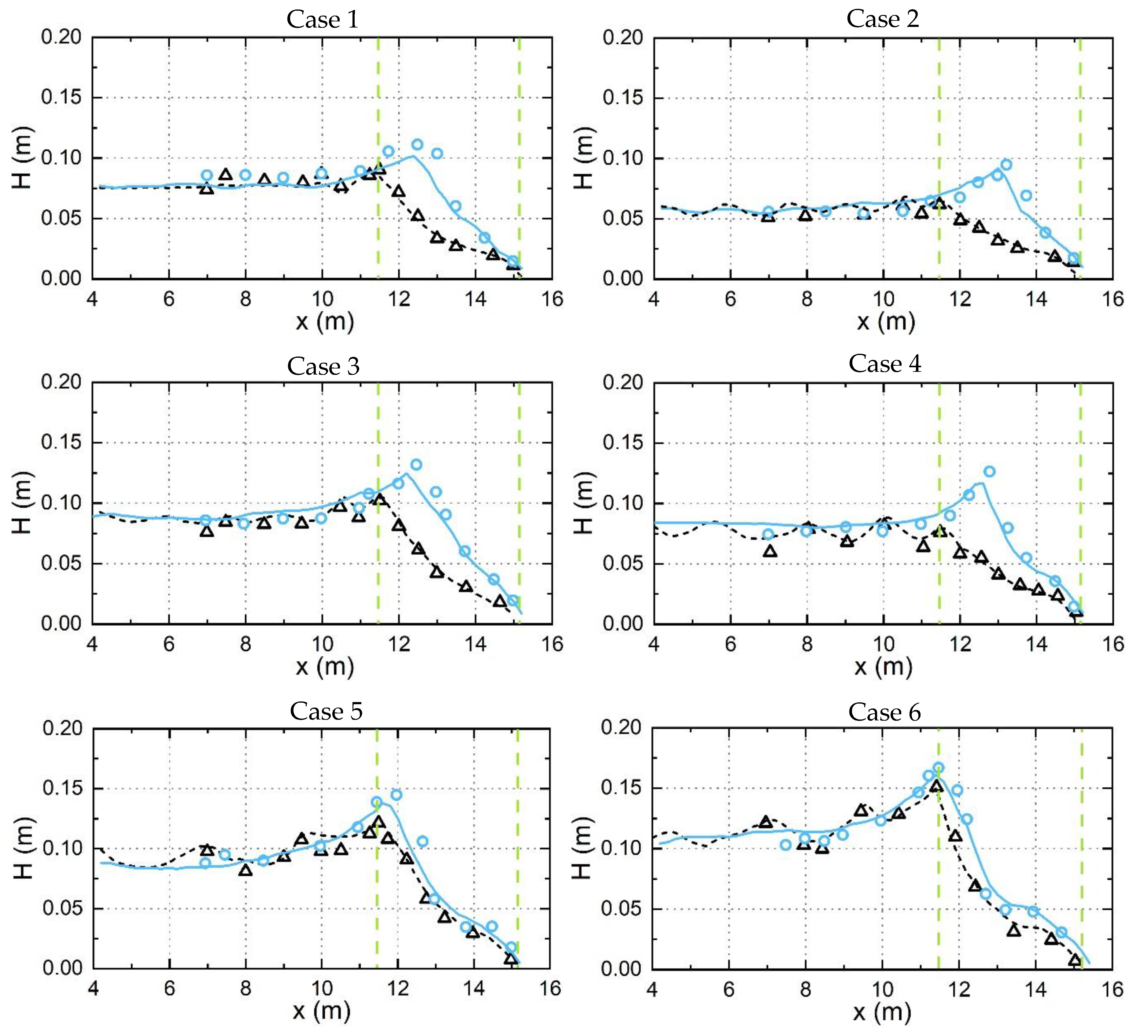
Figure 5 shows the model-data comparisons of wave height evolution without and with emerged vegetation. The solid and dashed lines correspond to the numerical results without and with vegetation. The circles represent the experimental data for no vegetation, and the triangles, for the emerged vegetation. The calculated wave height is averaged over five wave-periods after the water surface reaches the equilibrium oscillations. When there is no vegetation, the wave energy dissipation on the slope is completely due to the wave breaking, which is simulated by the multiphase - SST model. It is shown that the present model is capable of modeling wave shoaling and breaking. The wave breaking point is well predicted by the present model, except the wave height is underestimated at the breaking point. The wave reflection without vegetation is not obvious in all cases because most wave energy dissipates by wave breaking.
On the emerged vegetation slope, the wave height attenuation in the surf zone is also reasonably predicted. Clearly, the wave height with the vegetation is attenuated more rapidly than without the vegetation, suggesting that the vegetation effects on wave damping are significant. It can be seen that wave attenuation avoids increasing the wave height and prevent wave breaking, such as in case 2 and case 4. For case 5, the inclusion of the vegetation also moves the breaking point in the offshore direction. Furthermore, both measured and calculated profiles show significant oscillatory patterns, which is due to the interaction between the incident waves and the reflected waves from the vegetation patches. As the wave height and wave period of the incident wave increases, the oscillations of the wave height profile at the vegetation front become more obvious. It is also shown that the wave height and wave period will have significant influence on wave breaking behavior. The maximum wave height on the slope increases with the increase of the wave height and wave period. For case 2, the dominant wave energy dissipation is due to the vegetation. However, for case 6, the dominant wave energy dissipation is due to wave breaking, and the vegetation has a limited effect on the wave height.
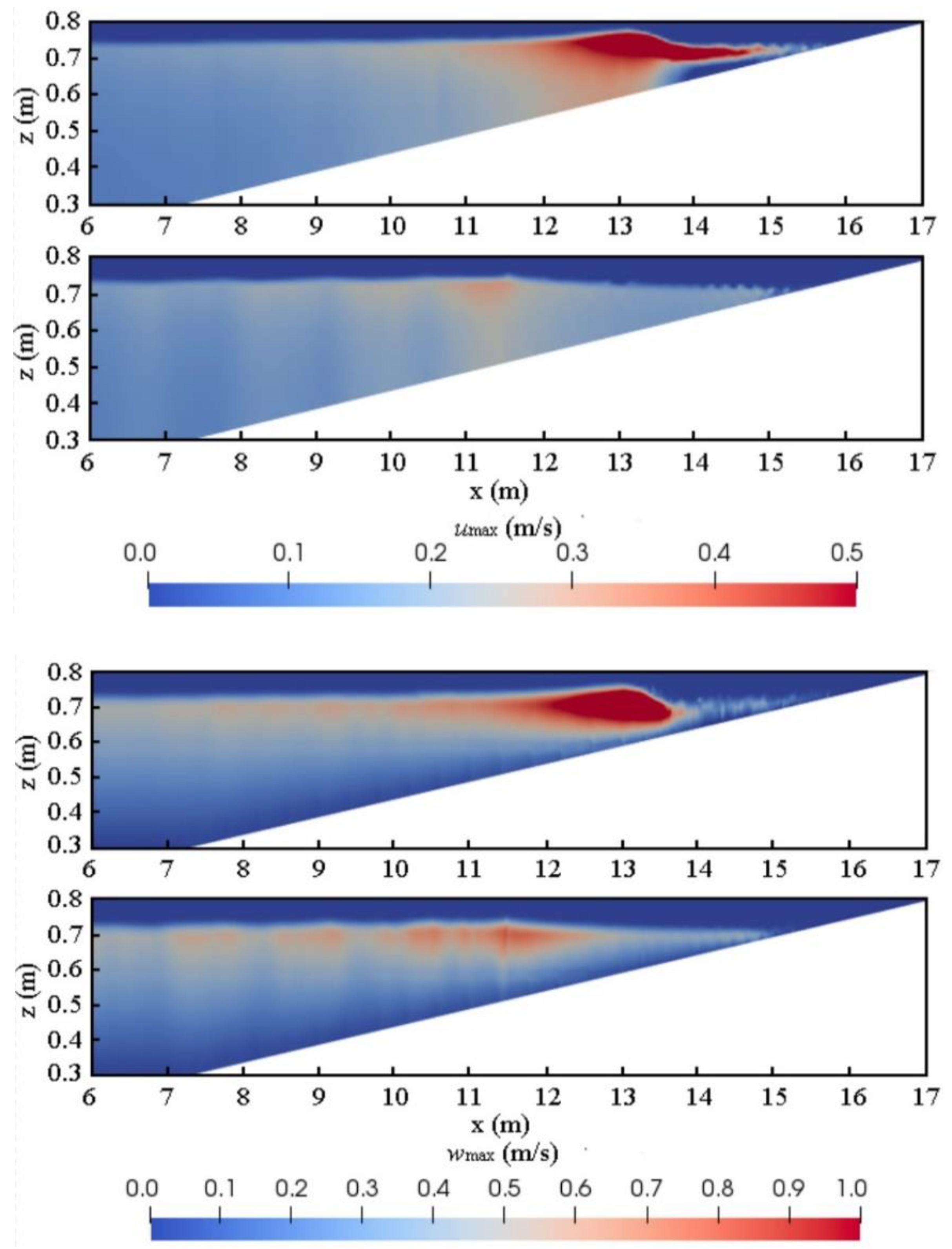
Figure 6 shows the maximum horizontal and vertical velocity fields in case 2. One is without vegetation and the other is with the emerged vegetation. A strong maximum horizontal velocity is observed near the shoreline if no vegetation is on the slope. With the enhanced resistance within the vegetation, the maximum horizontal velocity is noticeably reduced, compared to the unvegetated condition. In a similar way, the maximum vertical velocity is also much smaller near the shoreline. The velocity magnitude and its vertical distribution are important in relation to the coastal morphodynamics because the maximum velocity relates to the threshold motion of the sediment transport.
3.3. Regular Wave Propagation over the Shallow Meadow
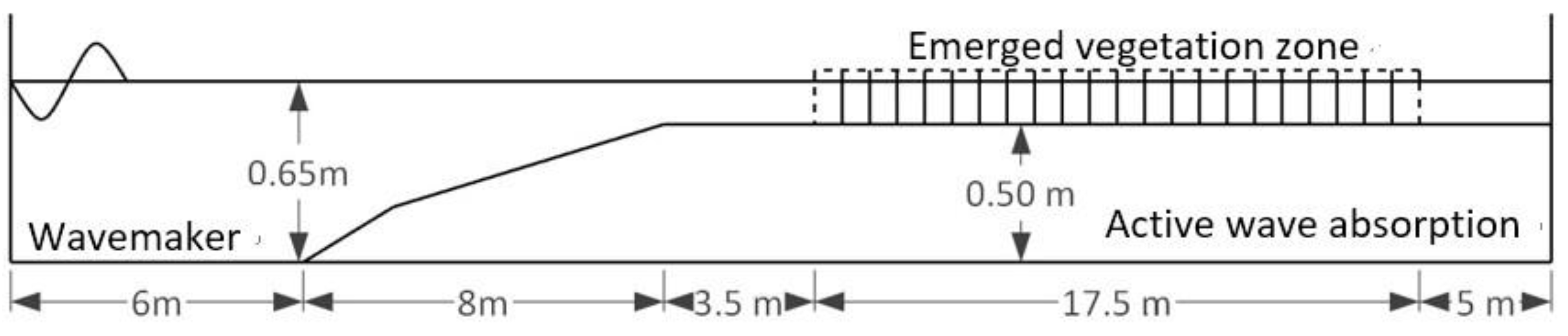
The experiments conducted at the Fluid Mechanics Laboratory at Delft University of Technology Phan et al. [10] are used to verify the model against the broken wave interaction with rigid vegetation on a shallow meadow. The laboratory flume was 40.0 m long, 1.0 m wide and 0.8 m deep. A wavemaker with an active wave absorption system was placed in the inlet boundary and a porous beach wave absorber was placed in the outlet boundary to dissipate the outgoing waves in order to reduce the reflection of incident waves. The rigid vegetation model was made of cylinder arrays with a diameter of 0.012 m. Two vegetation densities, which are N = 200 unit/m2 and N = 400 unit/m2 with staggered arrangement and tandem arrangement, respectively. The water depth was 0.65 m at the inlet boundary and 0.15 m at the meadow. According to Reeve et al. [34], second-order Stokes wave theory is chosen here for wave generation. Water surface elevations were measured upstream and inside of the vegetation zone. The experimental conditions used by the present model are given in Table 3. The drag coefficient is calibrated by comparing the wave heights of the measured data and the numerical results. It is noted that the calibrated drag coefficient used here is slightly different from the non-hydrostatic model Phan et al. [10]. This may be attributed to the wave boundaries and velocity profiles, as also reported by Chen et al. [37].
The numerical domain was set up to consistent with the experiment, as shown in Figure 7. The uniform grid discretization is used, having a grid size equal to 0.02 m in the horizontal direction and half of this value 0.01 m in the vertical one. In the surf zone, further mesh refinement in the horizontal direction was applied to keep aspect ratio of 1, i.e., Δx = Δz = 0.005 m. The final grid consists of 501,482 cells. The simulation time is 60 s and completing the simulation takes about 4 h in 24 cores (2.2 Ghz). For case 1, finer mesh of Δx = Δz = 0.005 m is needed near the free surface (between levels z = 0.6 m and 0.7 m) due to smaller wave height.
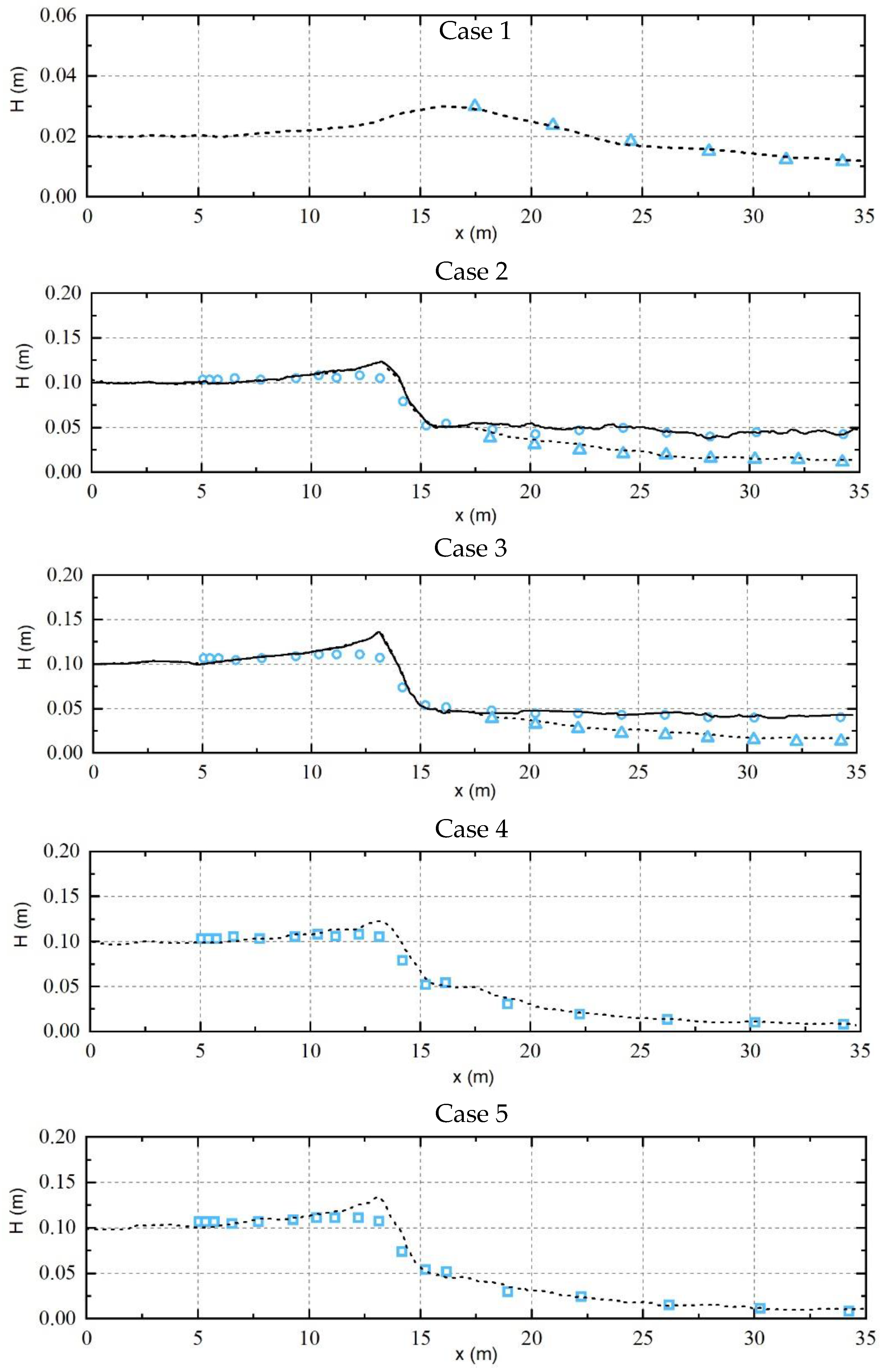
The measured and calculated wave heights are shown in Figure 8. The calculated wave heights are averaged over five wave-periods after the free surface reaches the equilibrium oscillations. The wave height evolution without the emerged vegetation is also shown in case 2 and case 3. The wave heights predicted by the model show good agreement with the experimental data for different wave conditions and vegetation density. For non-breaking waves, it is suggested that the wave height first slightly increases to about 0.03 m at the front edge of the vegetation (x = 17.5 m). After that, the wave height reduces to about 0.014 m over a span of 17.5 m in the vegetation zone as shown in Figure 8. For broken waves, the prediction exhibits a weak spatial oscillation after the wave breaking without the vegetation when wave period is 2 s. When the wave length is longer (case 3), the spatial oscillation predictions are reduced. This comparison shows that the absorbing boundary condition performs slightly better for shallow water waves than deep water conditions. This evolution leads to wave height attenuations up to around 80% for case 5 with the largest vegetation density.
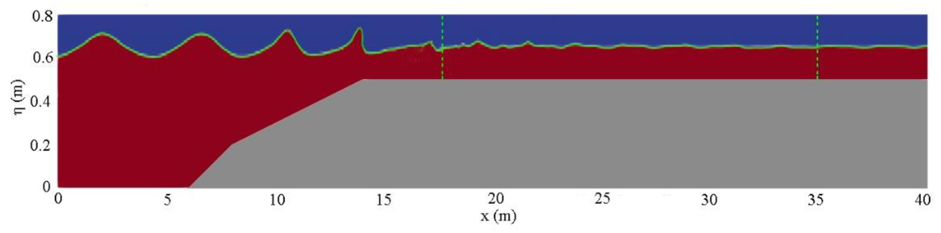
Figure 9 presents the snapshot of the free surface before waves start breaking as they approach the shoreline. The green dash lines show the location of the emerged vegetation. It can be found that the waveforms become asymmetric and the wave height increases due to wave shoaling effects on the slope.
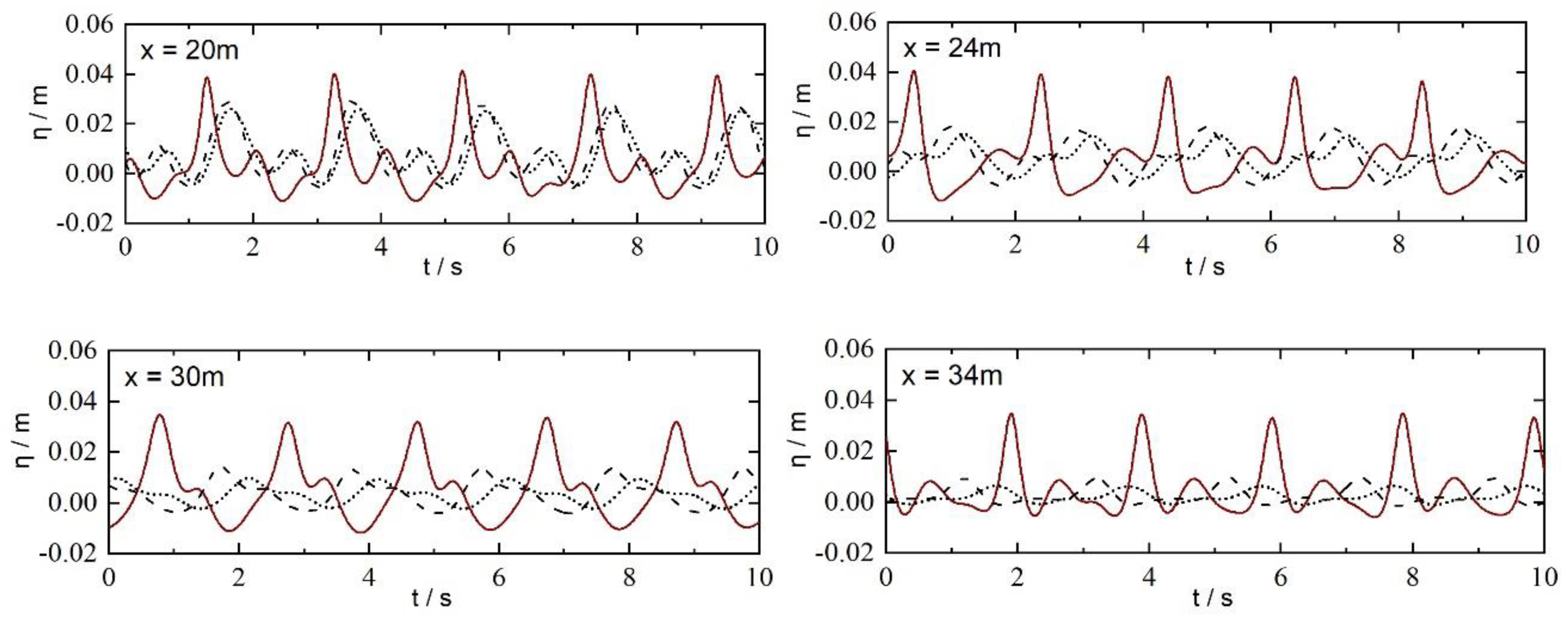
Free surface data without vegetation and with vegetation are compared to show the wave height attenuations over the vegetation zone. The vegetation density is N = 200 unit/m2, 400 unit/m2, and the wave period is 2.0 s. Wave gages are placed in the numerical wave tank at 20 m, 24 m, 30 m, and 34 m. The results are shown in Figure 10. Breaking waves on the slope reform on the shallow flat and gradually evolve into bore-like waves with multiple crest. Since the bore propagation speed is related to bore height, larger bores propagate faster and overtake the smaller ones. The nonlinearity, the wave crest being sharp and the wave trough being flat can be seen clearly.
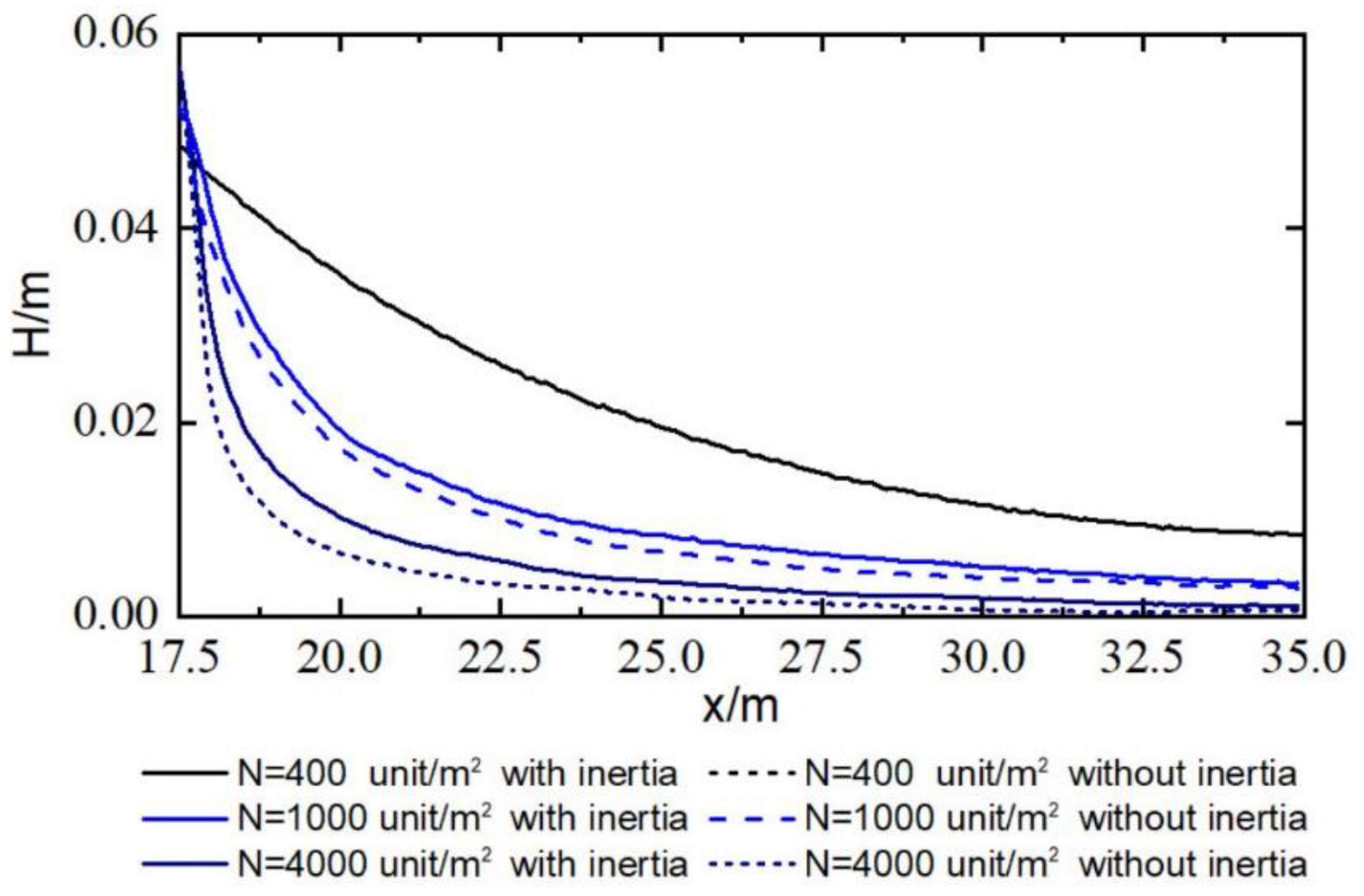
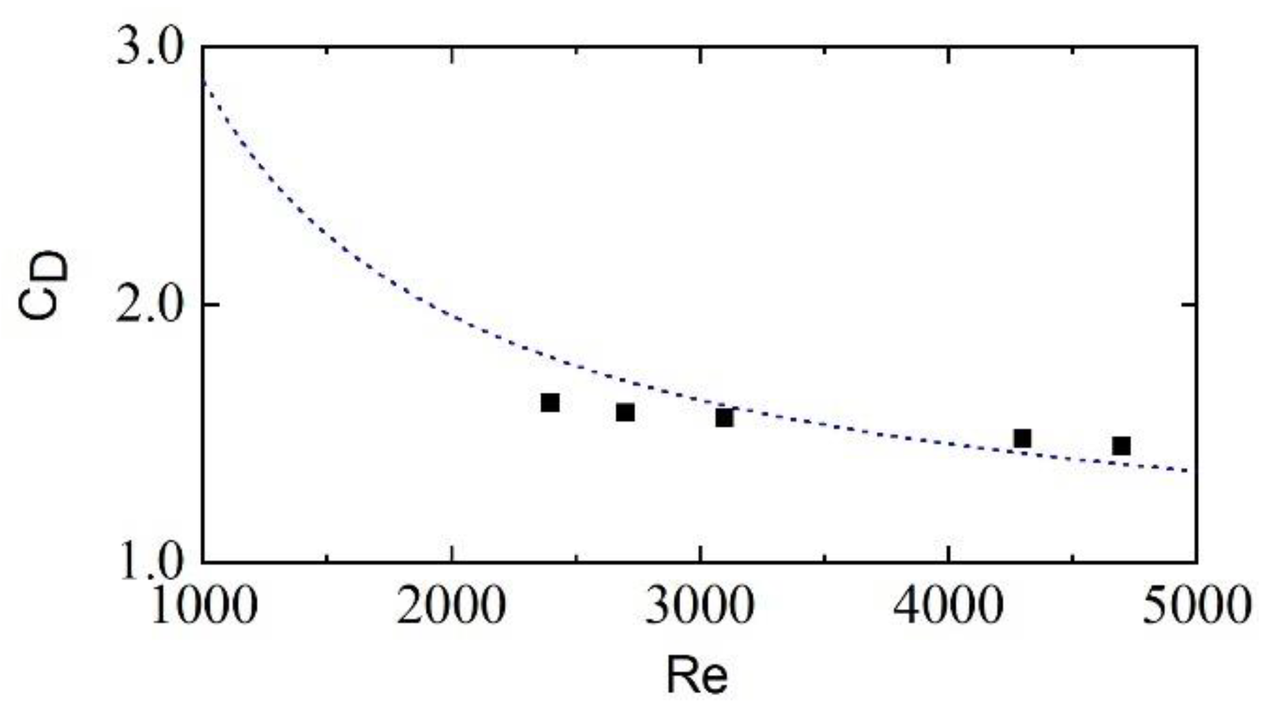
Another phenomenon that should be considered is the importance of the inertia force for broken waves. When applying linear theory, the work done by the inertia force is zero. Therefore, inertia force can be neglected. However, as the wave nonlinearity of the broken waves is generally high, the work done by the inertia force is nonzero, which has been validated with the experiments by Arnaud et al. [11]. The inertia force can become more important as the density of vegetation increases because the inertia force is proportional to the ratio of the vegetation area to the water field (e.g., ). As there are no experimental data available, an empirical relationship between the drag coefficient and Reynold number () proposed by Maza et al. [24] is used to determine the drag coefficient, this formula is expressed as Kobayashi [38] form,
where with is the characteristic velocity defined as the maximum horizontal velocity at the free surface of the first vegetation. The fitting value is .
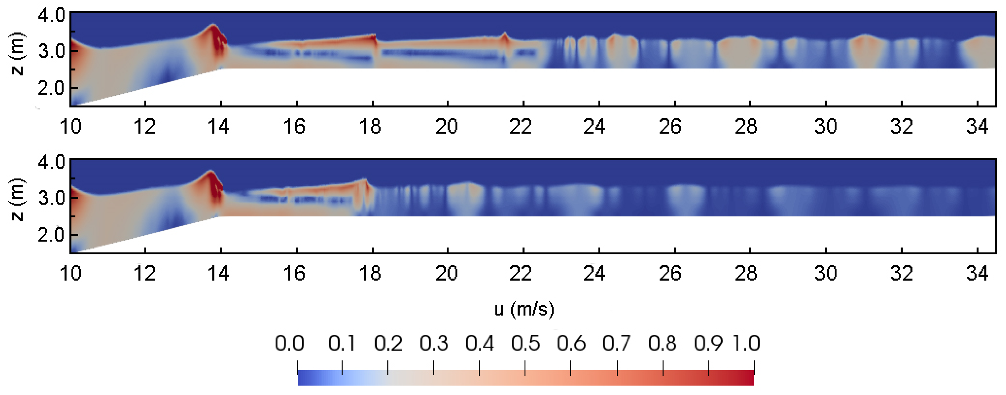
Figure 11 shows the calculated wave heights using both without and with the inertia force. When the vegetation is set as 400 unit/m2, the results are almost identical. However, when the vegetation is set as 4000 unit/m2, the difference arises as the inertia force reduces the wave damping induced by the vegetation. Therefore, the inertia force cannot be negligible when wave nonlinearity is high in the dense vegetation fields. It can be also seen that the wave height is decreased nonlinearly with the increase of the wave propagating distance, and nonlinearity is more obvious for the vegetation with a higher stem density. Most of the wave energy is damped by a span of the first 5 m in the vegetation. Figure 12 demonstrates that the snapshot of the velocity magnitude fields without vegetation and with vegetation, N = 400 unit/m2. Obviously, the existence of the vegetation does not affect the velocity distribution before the vegetation zone while the velocity reduces significantly inside it.
4. Discussion
Besides the numerical model used in this work, direct 3D numerical models, which consider each part of the vegetation individually and discretized their topography into a computational domain, have been gradually used in literature [15]. This can be easily extended within the present model by applying finer meshes at the location of vegetation patches. However, it is reasonable to make compromises between the accuracy of the results and computational efficiency. On the one hand, compared to direct models, this model can save much CPU time and obtain satisfactory results if the drag coefficient is determined properly. On the other hand, RANS models have taken into account the turbulence of wave breaking and the vegetation, which should reduce the overestimation of the wave height and the deviation of free surface [29]. When compared with the non-hydrostatic model, there is an improvement. First, the present model includes the energy dissipation caused by air that the experiments were carried out with. As a result, for the case of wave breaking, the free surface tracked by VOF method does not need to be continuous. It means that the splashed water into the air and the trapped air bubbles can also be handled with. Second, the high degrees of freedom to generates meshes containing hexahedra and split-hexahedra from triangulated surface geometries make it possible to treat the slope bathymetry more properly.
It has to be mentioned that there are still some limitations in simulating breaking waves with the vegetation. For example, the drag coefficient is dependent on a lot of factors, such as wave parameters and vegetation configurations, which will be discussed later. Moreover, there is no agreement in which turbulence model is the best one to be used, since their advantages usually come with particular shortcomings, as shown in Brown [28]. When considering the turbulence effects of the vegetation, the empirical constants in turbulence models are directly from non-breaking cases in other studies Hiraoka et al. [3] due to the lack of experimental data. The present model may sometimes underestimate the wave height after the wave breaking point (e.g., in experiments by Wu et al. [36]), depending on the wave conditions and bathymetry.
The determination of the drag coefficient remains the main issue that needs to be addressed. To the authors’ knowledge, the derivation of theoretical expressions for the drag coefficient does not exist. The common approach is to establish an empirical relationship between the drag coefficient and other dimensionless parameters, such as Reynold number () or Keulegan-Carpenter number (), by the experiments. Generally, the drag coefficient decreases when and increase. For experiments by Iimura et al. [8], however, no empirical formula can be found since few of them are particularly for the solitary waves. For experiments by Wu et al. [36], Tanino et al. [39] proposed a formula for the drag coefficient of emerged rigid cylinders to establish the relationship between the drag coefficients and . The validation of drag coefficients has already been done by Wu et al. [36] and will not be discussed here. This formula is valid in the range , which is not suitable for Phan et al. experiments (). For experiments by the Phan et al. [10], the empirical formula proposed by Maza et al. [24], as mentioned before, is used to fit calibrated drag coefficients in their experiments. The calibrated drag coefficients compared with the formulas are shown in Figure 13.
As a result, although the drag coefficients have been studied in detail and there are numerous experiments on the topic for the past decades, a general expression to estimate the drag coefficient suitable in most cases is not available. It is important to keep in mind that the existing empirical formulas still do not fit well with the drag coefficients obtained from the experiments.
5. Conclusions
In this paper, a VOF-based RANS model is employed to investigate the wave dissipation due to the wave breaking and the emerged vegetation. The model is achieved using the OpenFOAM code. The multiphase - SST turbulence model is adopted to simulate wave breaking. The effects of the vegetation are modeled by the drag and inertia source terms in the momentum equations. The model is validated using three laboratory experiments of solitary and monochromatic wave propagation through vegetation field. Despite some assumptions have been made (e.g., constant drag and inertia coefficients along the vegetation field and over time, the porosity and the flexibility of the vegetation are ignored), the model is capable of simulating nonbreaking, breaking and broken wave attenuation by the emerged vegetation with adequate coefficients. On the vegetated slope, wave attenuation by the vegetation avoids wave steepening and prevents wave breaking. It can be concluded that the wave energy dissipation rate for breaking waves is dependent on the wave height and wave period, the wave reflection increases with an increase of the wave period. For broken waves, strong wave nonlinearity is observed after wave breaking. The inertia force within denser vegetation has a negative effect on energy dissipation and the wave attenuation can be overestimated if the inertia force is neglected.
Natural vegetation fields are far more complicated than can be mimicked in laboratory experiments and numerical models. The vegetation root and canopy in the vegetation zone can also affect the wave attenuation. For the purpose of quantifying physical vegetation properties, a detailed vegetation model including the root and canopy should be presented in later work. It should be also noted that the present model is only validated by laboratory experiments, extra field data are needed to analyze the reliability of field modeling results.
Author Contributions
X.Z. built the numerical model; X.Z. and L.Z. performed the numerical simulation; X.Z., L.Z. and J.Z. analyzed the data; X.Z. and L.Z. wrote the paper.
Funding
This research was funded by the National Natural Science Foundation of China grant number (1157213).
Acknowledgments
The authors to appreciate all the developers and contributors to the open-source code and thank the users in the OpenFOAM forum, which has helped to present the details of our implementation.
Conflicts of Interest
The authors declare no conflict of interest.
References
- Paul, T.; Kevin, H.; David, T. Wave attenuation by emergent wetland vegetation. In Proceedings of the 27th International Conference on Coastal Engineering, Sydney, Australia, 16–21 July 2000; pp. 865–877. [Google Scholar]
- Harada, K.; Imamura, F.; Hiraishi, T. Advances in hydraulics and water engineering Volumes I. In Proceedings of the 13th Iahr-apd Congress, Singapore, 6–8 August 2002; World Scientific: Singapore; pp. 910–915.
- Hiraoka, H.; Ohashi, M.A. (k–ε) turbulence closure model for plant canopy flows. J. Wind Eng. Ind. Aerodyn. 2008, 96, 2139–2149. [Google Scholar] [CrossRef]
- Chen, H.; Zou, Q.P. Eulerian-Lagrangian flow-vegetation interaction model using immersed boundary method and OpenFOAM. Adv. Water Resour. 2019, 126, 176–192. [Google Scholar] [CrossRef]
- Dalrymple, R.A.; Kirby, J.T.; Hwang, P.A. Wave Diffraction Due to Areas of Energy Dissipation. J. Waterw. Port Coast. Ocean Eng. 1984, 110, 67–79. [Google Scholar] [CrossRef]
- Mendez, F.J.; Losada, I.J. An empirical model to estimate the propagation of random breaking and nonbreaking waves over vegetation fields. Coast. Eng. 2004, 51, 103–118. [Google Scholar] [CrossRef]
- Stratigaki, V.; Manca, E.; Prinos, P.; Losada, I.J.; Lara, J.; Sclavo, M.; Amos, C.; Caceres, I.; Sánchez-Arcilla, A. Large-Scale experiments on wave propagation over posidonia oceanica. J. Hydraul. Res. 2011, 49, 31–43. [Google Scholar] [CrossRef]
- Iimura, K.; Tanaka, N. Numerical simulation estimating effects of tree density distribution in coastal forest on tsunami mitigation. Ocean Eng. 2012, 54, 223–232. [Google Scholar] [CrossRef]
- Koftis, T.; Prinos, P.; Stratigaki, V. Wave damping over artificial Posidonia oceanica meadow: A large-scale experimental study. Coast. Eng. 2013, 73, 71–83. [Google Scholar] [CrossRef]
- Phan, K.L.; Stive, M.J.F.; Zijlema, M.; Truong, H.S.; Aarninkhof, S.G.J. The effects of wave non-linearity on wave attenuation by vegetation. Coast. Eng. 2019, 147, 63–74. [Google Scholar] [CrossRef]
- Arnaud, G.; Rey, V.; Touboul, J.; Sous, D.; Molin, B.; Gouaud, F. Wave propagation through dense vertical cylinder arrays: Interference process and specific surface effects on damping. Appl. Ocean Res. 2017, 65, 229–237. [Google Scholar] [CrossRef]
- Houser, C.; Trimble, S.; Morales, B. Influence of blade flexibility on the drag coefficient of aquatic vegetation. Estuaries Coasts 2015, 38, 569–577. [Google Scholar] [CrossRef]
- Luhar, M.; Nepf, H.M. Wave-induced dynamics of flexible blades. J. Fluids Struct. 2016, 61, 20–41. [Google Scholar] [CrossRef] [Green Version]
- Cavallaro, L.; Viviano, A.; Paratore, G.; Foti, E. Experiments on surface waves interacting with flexible aquatic vegetation. Ocean Sci. J. 2018, 53, 461–474. [Google Scholar] [CrossRef] [Green Version]
- Maza, M.; Lara, J.L.; Losada, I.J. Tsunami wave interaction with mangrove forests: A 3-D numerical approach. Coast. Eng. 2015, 98, 33–54. [Google Scholar] [CrossRef]
- Strusinska-Correia, A.; Husrin, S.; Oumeraci, H. Tsunami damping by mangrove forest: A laboratory study using parameterized trees. Nat. Hazards Earth Syst. Sci. 2013, 13, 483. [Google Scholar] [CrossRef] [Green Version]
- Knutson, P.L.; Brochu, R.A.; Seelig, W.N.; Inskeep, M. Wave damping in Spartina alterniflora marshes. Wetlands 1982, 2, 87–104. [Google Scholar] [CrossRef]
- Paul, M.; Bouma, T.; Amos, C. Wave Attenuation by Submerged Vegetation: Combining the Effect of Organism Traits and Tidal Current. Mar. Ecol. Prog. Ser. 2012, 444, 31–41. [Google Scholar] [CrossRef] [Green Version]
- Vanegas, G.C.A.; Osorio, A.F.; Urrego, L.E. Wave dissipation across a Rhizophora mangrove patch on a Colombian Caribbean Island: An experimental approach. Ecol. Eng. 2019, 130, 271–281. [Google Scholar] [CrossRef]
- Suzuki, T.; Zijlema, M.; Burger, B.; Meijer, M.C.; Narayan, S. Wave dissipation by vegetation with layer schematization in SWAN. Coast. Eng. 2012, 59, 64–71. [Google Scholar] [CrossRef]
- Vo-Luong, P.; Massel, S. Energy dissipation in non-uniform mangrove forests of arbitrary depth. J. Mar. Syst. 2008, 74, 603–622. [Google Scholar] [CrossRef]
- Augustin, L.N.; Irish, J.L.; Lynett, P. Laboratory and numerical studies of wave damping by emergent and near-emergent wetland vegetation. Coast. Eng. 2009, 56, 332–340. [Google Scholar] [CrossRef]
- Suzuki, T.; Hu, Z.; Kumada, K.; Phan, L.K.; Zijlema, M. Non-hydrostatic modeling of drag, inertia and porous effects in wave propagation over dense vegetation fields. Coast. Eng. 2019, 149, 49–64. [Google Scholar] [CrossRef]
- Maza, M.; Lara, J.L.; Losada, I.J. A coupled model of submerged vegetation under oscillatory flow using Navier–Stokes equations. Coast. Eng. 2013, 80, 16–34. [Google Scholar] [CrossRef]
- Chen, X.; Chen, Q.; Zhan, J.; Liu, D. Numerical simulations of wave propagation over a vegetated platform. Coast. Eng. 2016, 110, 64–75. [Google Scholar] [CrossRef] [Green Version]
- Ting, F.C.K.; Kirby, J.T. Observation of undertow and turbulence in a laboratory surf zone. Coast. Eng. 1994, 24, 51–80. [Google Scholar] [CrossRef]
- Nepf, H.M. Drag, turbulence, and diffusion in flow through emergent vegetation. Water Resour. Res. 1999, 35, 479–489. [Google Scholar] [CrossRef]
- Brown, S.A.; Greaves, D.M.; Magar, V.; Conley, D.C. Evaluation of turbulence closure models under spilling and plunging breakers in the surf zone. Coast. Eng. 2016, 114, 177–193. [Google Scholar] [CrossRef] [Green Version]
- Devolder, B.; Troch, P.; Rauwoens, P. Performance of a buoyancy-modified k-ω and k-ω SST turbulence model for simulating wave breaking under regular waves using OpenFOAM®. Coast. Eng. 2018, 138, 49–65. [Google Scholar] [CrossRef] [Green Version]
- Lubin, P.; Vincent, S.; Abadie, S.; Caltagirone, J.P. Three-dimensional large eddy simulation of air entrainment under plunging breaking waves. Coast. Eng. 2006, 53, 631–655. [Google Scholar] [CrossRef] [Green Version]
- Lubin, P.; Glockner, S.; Kimmoun, O.; Branger, H. Numerical study of the hydrodynamics of regular waves breaking over a sloping beach. Eur. J. Mech. 2011, 30, 552–564. [Google Scholar] [CrossRef] [Green Version]
- Tang, J.; Shen, S.; Wang, H. Numerical model for coastal wave propagation through mild slope zone in the presence of rigid vegetation. Coast. Eng. 2015, 97, 53–59. [Google Scholar] [CrossRef]
- Morison, J.R.; Johnson, J.W.; Schaaf, S.A. The force exerted by surface waves on piles. J. Pet. Technol. 1950, 2, 149–154. [Google Scholar] [CrossRef]
- Reeve, D.; Chadwick, A.; Fleming, C. Coastal Engineering: Processes, Theory and Design Practice; CRC Press: Boca Raton, FL, USA, 2012. [Google Scholar]
- Menter, F.R. Two-equation eddy-viscosity turbulence models for engineering applications. AIAA J. 1994, 32, 1598–1605. [Google Scholar] [CrossRef] [Green Version]
- Wu, W.; Ozeren, Y.; Wren, D.; Chen, Q.; Zhang, G.; Holland, M.; Marsooli, R.; Lin, Q.; Jadhav, R.; Parker, K.R.; et al. Investigation of Surge and Wave Reduction by Vegetation: Phase II Report for SERRI Project; The University of Missippi: Oxford, MS, USA, 2012. [Google Scholar]
- Chen, H.; Liu, X.; Zou, Q.P. Wave-driven flow induced by suspended and submerged canopies. Adv. Water Resour. 2019, 123, 160–172. [Google Scholar] [CrossRef]
- Kobayashi, N.; Raichle, A.W.; Asano, T. Wave Attenuation by Vegetation. J. Waterw. Port Coastal Ocean Eng. 1993, 119, 30–48. [Google Scholar] [CrossRef]
- Tanino, Y.; Nepf, H.M. Laboratory investigation of mean drag in a random array of rigid, emergent cylinders. J. Hydraul. Eng. 2008, 134, 34–41. [Google Scholar] [CrossRef]
Figure 1.
Sketch of the wave tank for experiments by Iimura et al. [8] (case 1).
Figure 1.
Sketch of the wave tank for experiments by Iimura et al. [8] (case 1).

Figure 2.
Calculated (dashed line) and experimental (triangle) maximum free surface, , along the vegetation patch. x denotes the longitudinal distance from the upstream edge of the vegetation patch, vertical green dashed lines denote the boundaries of the vegetation area.
Figure 2.
Calculated (dashed line) and experimental (triangle) maximum free surface, , along the vegetation patch. x denotes the longitudinal distance from the upstream edge of the vegetation patch, vertical green dashed lines denote the boundaries of the vegetation area.

Figure 3.
Free surface, time series at the end of the vegetation in case 3. Experiment data (blue dots) and numerical results (black dash line)
Figure 3.
Free surface, time series at the end of the vegetation in case 3. Experiment data (blue dots) and numerical results (black dash line)

Figure 4.
Sketch of the wave tank for experiments by Wu et al. [36].
Figure 4.
Sketch of the wave tank for experiments by Wu et al. [36].

Figure 5.
Calculated (solid line: without vegetation, dashed line: with vegetation) and Wu et al. [36] experimental (circle: without vegetation, triangle: with vegetation) wave height, H, inside the vegetation patch. x denotes the longitudinal distance from the wavemaker boundary, vertical green dashed lines denote the boundaries of the vegetation area.

Figure 6.
The Eulerian maximum horizontal () and vertical () velocity field contour in case 2. Upper (no vegetation) Lower (with emerged vegetation).
Figure 6.
The Eulerian maximum horizontal () and vertical () velocity field contour in case 2. Upper (no vegetation) Lower (with emerged vegetation).

Figure 7.
Sketch of the wave tank for Phan et al. [10] experiments.
Figure 7.
Sketch of the wave tank for Phan et al. [10] experiments.

Figure 8.
Calculated (solid line: without vegetation, dash line: with vegetation) and Phan experimental (circles: without vegetation, triangle: N = 200 unit/m2, square: N = 400 unit/m2) wave height, H, inside the vegetation patch. x denotes the longitudinal distance from the wavemaker boundary.
Figure 8.
Calculated (solid line: without vegetation, dash line: with vegetation) and Phan experimental (circles: without vegetation, triangle: N = 200 unit/m2, square: N = 400 unit/m2) wave height, H, inside the vegetation patch. x denotes the longitudinal distance from the wavemaker boundary.

Figure 9.
Snapshot of the free surface, , (green solid line) when H = 1.0 m, T = 2.0 s with N = 400 unit/m2, vertical green dashed lines denote the boundaries of the vegetation area.
Figure 9.
Snapshot of the free surface, , (green solid line) when H = 1.0 m, T = 2.0 s with N = 400 unit/m2, vertical green dashed lines denote the boundaries of the vegetation area.

Figure 10.
Free surface, , time series measured by wave gauges with H = 0.1 m, T = 2.0 s inside the vegetation. No vegetation (solid line), N = 200 unit/m2 (dash line) and N = 400 unit/m2 (dot line).
Figure 10.
Free surface, , time series measured by wave gauges with H = 0.1 m, T = 2.0 s inside the vegetation. No vegetation (solid line), N = 200 unit/m2 (dash line) and N = 400 unit/m2 (dot line).

Figure 11.
Spatial distribution of wave height, H, for reformed waves after wave breaking in the presence of emerged vegetation with different vegetation densities.
Figure 11.
Spatial distribution of wave height, H, for reformed waves after wave breaking in the presence of emerged vegetation with different vegetation densities.

Figure 12.
Snapshot of the velocity magnitude when H = 1.0 m, T = 2.0 s without vegetation (Upper) and with N = 400 unit/m2 (Lower).
Figure 12.
Snapshot of the velocity magnitude when H = 1.0 m, T = 2.0 s without vegetation (Upper) and with N = 400 unit/m2 (Lower).

Figure 13.
Variation of estimated drag coefficient with Reynolds number ().


Table 1.
Experiment study by emerged vegetation over the slope Iimura et al. [8].
Table 1.
Experiment study by emerged vegetation over the slope Iimura et al. [8].
| Case | Incident Wave Height Hi (m) | Vegetation Width w (m) | Vegetation Density N (unit/m2) | Calibrated CD |
|---|---|---|---|---|
| 1 | 0.0314 | 1.0 | 462 | 0.71 |
| 2 | 0.0314 | 0.36 | 1283 | 0.66 |
| 3 | 0.0314 | 0.04 | 11,547 | 1.73 |
| 4 | 0.0314 | 0.08, 0.32 | 2887, 722 | 0.83, 0.84 |
| 5 | 0.0314 | 0.32, 0.08 | 722, 2887 | 0.76, 0.92 |
Table 2.
Experiment study by emerged vegetation on the meadow Wu et al. [36].
Table 2.
Experiment study by emerged vegetation on the meadow Wu et al. [36].
| Case | Incident Wave Height Hi (m) | Wave Period T (s) | Vegetation Density N (unit/m2) | Calibrated CD |
|---|---|---|---|---|
| 1 | 0.0873 | 1.2 | 3182 | 1.7 |
| 2 | 0.0533 | 1.8 | 3182 | 1.7 |
| 3 | 0.0830 | 1.8 | 3182 | 1.7 |
| 4 | 0.0782 | 2.4 | 3182 | 1.7 |
| 5 | 0.0735 | 3.0 | 3182 | 1.7 |
| 6 | 0.0853 | 3.0 | 3182 | 1.7 |
Table 3.
Experiment study by emerged vegetation on the meadow Phan et al. [10].
Table 3.
Experiment study by emerged vegetation on the meadow Phan et al. [10].
| Case | Incident Wave Height Hi (m) | Wave Period T (s) | Vegetation Density N (unit/m2) | Calibrated CD |
|---|---|---|---|---|
| 1 | 0.02 | 2.0 | 200 | 1.62 |
| 2 | 0.1 | 2.0 | 200 | 1.58 |
| 3 | 0.1 | 3.0 | 200 | 1.56 |
| 4 | 0.1 | 2.0 | 400 | 1.45 |
| 5 | 0.1 | 3.0 | 400 | 1.41 |
© 2019 by the authors. Licensee MDPI, Basel, Switzerland. This article is an open access article distributed under the terms and conditions of the Creative Commons Attribution (CC BY) license (http://creativecommons.org/licenses/by/4.0/).
Share and Cite
MDPI and ACS Style
Zou, X.; Zhu, L.; Zhao, J. Numerical Simulations of Non-Breaking, Breaking and Broken Wave Interaction with Emerged Vegetation Using Navier-Stokes Equations. Water 2019, 11, 2561. https://doi.org/10.3390/w11122561
AMA Style
Zou X, Zhu L, Zhao J. Numerical Simulations of Non-Breaking, Breaking and Broken Wave Interaction with Emerged Vegetation Using Navier-Stokes Equations. Water. 2019; 11(12):2561. https://doi.org/10.3390/w11122561
Chicago/Turabian StyleZou, Xuefeng, Liangsheng Zhu, and Jun Zhao. 2019. "Numerical Simulations of Non-Breaking, Breaking and Broken Wave Interaction with Emerged Vegetation Using Navier-Stokes Equations" Water 11, no. 12: 2561. https://doi.org/10.3390/w11122561
Note that from the first issue of 2016, this journal uses article numbers instead of page numbers. See further details here.