Experimental Investigation of Coherent Vortex Structures in a Backward-Facing Step Flow


1
State Key Laboratory of Hydrology-Water Resources and Hydraulic Engineering, Nanjing Hydraulic Research Institute, Nanjing 210029, China
2
Department of Civil Engineering and Mechanics, University of Wisconsin-Milwaukee, Milwaukee, WI 53201, USA
*
Authors to whom correspondence should be addressed.
Water 2019, 11(12), 2629; https://doi.org/10.3390/w11122629
Submission received: 14 October 2019
/
Revised: 23 November 2019
/
Accepted: 10 December 2019
/
Published: 13 December 2019
(This article belongs to the Special Issue Advances in Hydraulics and Hydroinformatics)
Abstract
:Coherent vortex structures (CVS) are discovered for more than half a century, and they are believed to play a significant role in turbulence especially for separated flows. An experimental study is conducted for a pressured backward-facing step flow with Reynolds number (Reh) being 4400 and 9000. A synchronized particle image velocimetry (PIV) system is developed for measurement of a wider range of velocity fields with high resolution. The CVS are proved to exist in the separation-reattachment process. For their temporal evolution, a life cycle is proposed that vortices form in the free shear layer, develop with pairings and divisions and finally shed at the reattachment zone, and sometimes new vortical structures are restructured with recovery of flow pattern. The CVS favor the free shear layer with frequent pairings and divisions particularly at the developing stage around x/h = 2~5 (x: distance from the step in flow direction, h: step height), which may contribute to the high turbulent intensity and shear stress there. A critical distance is believed to exist among CVS, which affects their amalgamation (pairing) and division events. Statistics show that the CVS are well organized in spatial distribution and show specific local features with the flow structures distinguished. The streamwise and vertical diameters (Dx and Dy) and width to height ratio (Dx/Dy) all obey to the lognormal distribution. With increase of Reh from 4400 to 9000, Dx decreases and Dy increases, but the mean diameter (D=0.5 × (Dx + Dy)) keeps around (0.28~0.29) h. As the increase of Reh, the vortical shape change toward a uniform condition, which may be contributed by enhancement of the shear intensity.
1. Introduction
Flow separation is common in various applications in our daily life (airfoils at large attack angle, spoiler flows, flow behind a vehicle, flow inside a combustor/condenser, flows in an enlarged pipe or a channel with steps, and flows around a boat or a building, etc.). Backward-facing step (BFS) is one basic model and fundamental in geometry and engineering design [1,2,3,4,5]. Flow separation behind the step changes transport of momentum, heat, and mass, and increases fluid mixing [6], and it also possibly leads to additional flow resistance and noise, and even for stalling of an aircraft under critical conditions. In a combustor or chamber, effective mixing is preferred and can be designed with detailed BFS geometric considerations [5,7,8,9]. In addition, the enlarged boundary in a pipe or channel sometimes generates unfavorable boundary erosion and structural vibration, and sometimes energy dissipation caused by structural changes in hydraulic engineering arouses people’s curiosity. In field of scouring downstream of a structure, motions and fluctuations of the vortices will cause sediment transport and river-bed scour [10]. However, because of the irregularity and complexity of turbulence, the flow characteristics, various mechanisms, and controlling studies on this flow are still worth further efforts with developments of measurement techniques [1,2,3,4,5,11]. In particular, coherent vortex structures (CVS) are discovered to play an important role and may be a promising way to investigate this flow [1,3,4,5,6,11,12,13,14,15,16]. However, quantitative studies of the CVS (e.g., the conception, identification, structure, scale, and evolution, etc.,) are deficient, and it is still difficult to fully understand the hydrodynamic mechanisms and unsteady interactions in many applications (e.g., pipe cavitation, earth dam break, riverbed and bank erosion, sand dune evolution, and energy dissipation).
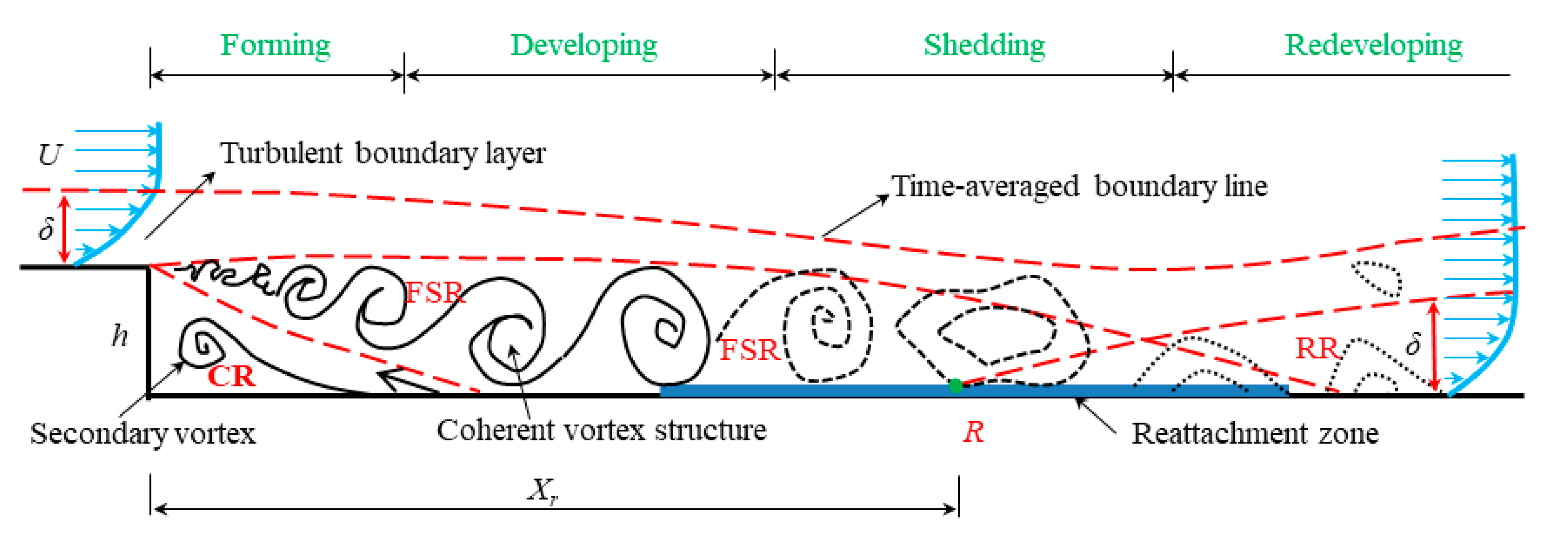
Figure 1 shows the typical flow structures in a two-dimensional BFS. Flow separates at the step edge (step height, h) and reattaches the bottom wall at some distance downstream, forming a recirculation region behind the step. This process consists of most physical features of a separation-reattachment flow, such as the free shear layer, the reattachment zone, and the redeveloping boundary layer [5,11,13,16,17,18,19]. The recirculation region is extensively studied in the previous researches. Length of this region (recirculation length, Xr) keeps a relative stable value of (7 ± 1) h for a developed turbulent flow, while it increases for a laminar flow and decreases for a transitional flow with the increase of Reynolds number [20]. The time-averaged flow structure is believed to be stable in a developed turbulent flow such as the free shear region (FSR), the corner region (CR), the redeveloping region (RR), and the reattachment zone [11]. These regions show various flow characteristics. The FSR is generated from the step top corner with strong shear intensity and finally limited by the bottom wall. The CR is located at the step corner with a secondary backflow. The RR shows a new development for the turbulent boundary layer after reattachment. The reattachment zone is defined as the locus of points, where the limiting streamline of the time-averaged flow rejoins the surface [21]. For the temporal flow, perturbation of the step generates successive CVS which promotes the fluid mixing and intensifies the unsteady interaction. The CVS shows four typical developing stages with various characteristic frequencies in the flow direction: forming, developing, shedding, and redeveloping [11].
The complexities of BFS flows are summarized by Roos and Kegelman (1986) [12]: (1) development of CVS in the free shear layer; (2) substantial unsteadiness of the entire separated flow, especially near the reattachment zone and particularly at low frequencies; (3) slow relaxation to equilibrium of the reattached shear layer, and the third one is also related to the former two. Recent decades, researchers are working on the CVS and unsteady motions in the complex flows.
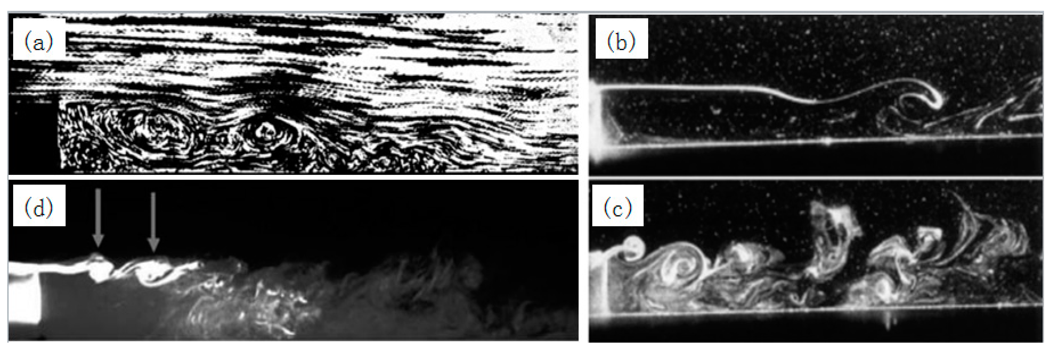
Flow visualization is first used to investigate this flow. Tani et al. (1961) [22] showed aluminum-power pictures of an instantaneous BFS flow and found that short exposure pictures reveal some distinct vortex structures (CVS) in the recirculation (Figure 2a), while pictures of long exposure only indicate something like that shown in the mean dividing streamlines. The CVS present formation, merging, and increasing irregularity with the increase of shear layer turbulence and persistence of the structures downstream of reattachment (Figure 2b–d) [6,14]. The CVS are believed to be rolled up in the strong shear layer, which grows with a vortex pairing mechanism until it approaches the reattachment zone [6,12,14,15,22]. In the reattachment zone, the CVS are torn roughly into two in the neighborhood of the reattachment point (R), where part of the flow is deflected upstream into the recirculation region to supply the entrainment and another part continues downstream [16]. McGuinness (1978) [23] believes that some CVS are swept upstream with the recirculating flow, while others proceed downstream. The fact that CVS move alternately up and downstream is also supported by the measurements of Chandrsuda (1975) [24] and Kim et al. (1978) [25]. In first part of the FSR, CVS and their evolution are usually explained by the Kelvin-Helmholtz instability that proposed in a plane mixing layer. However, BFS flow shows some differences [1,12]: (1) The free shear layer has a finite length due to the reattachment, which limits the development of the CVS; (2) The free shear layer supports an adverse pressure gradient and is curved; (3) Strong interaction between the unsteady shear layer and the reattachment wall generates substantial acoustic and convective disturbances, that feed back through the recirculation to influence the shear layer at separation. The peak value of turbulence intensity in a BFS flow is 10~20% higher than that of a plane mixing layer [1]. Additionally, local forcing with certain frequency is proved to contribute to amalgamation of the CVS and fluid mixing (Figure 2b,c), which also shortens Xr [6].
Various quantitative measurements are applied to obtain velocity or pressure information such as hot-wire, x-wires, hydrogen bubble, laser doppler velocimetry, and particle image velocimetry (PIV) [11,16,20,26,27,28,29,30]. Many of the measurements can only measure and analyze point-by-point characteristics or time-averaged flow fields information such as Xr, turbulent shear stress, turbulent intensity, backflow, and characteristic frequency, etc. Recent developments of experimental measurements and numerical simulations allowed in-depth investigation of the flow dynamics. For example, PIV makes it possible to obtain some velocity fields and flow structures with temporal vortical evolutions. Scarano et al. (1999) [29] investigate the trajectories and sizes of CVS with Reh = 5000, utilizing a pattern recognition analysis. They concluded that the length scale of the CVS ranges from 0.12 h to 0.44 h, and those with smaller diameters occur more frequently. They suggest that the clockwise CVS arise from a Kelvin–Helmholtz instability in the FSR, while the counter-clockwise CVS in the CR are due to a three-dimensional breakdown of the clockwise ones. Staggered vortex trains and pairings within the FSR are identified in the instantaneous PIV measurements by Kostas et al. (2002) [14]. They propose that the vortical interactions are most likely to contribute to the high Reynolds stresses and turbulent kinetic energy production. Furthermore, the CVS seem to be largely responsible for the persistence of the streamwise turbulent intensity (u’2) and the shear stress (u’v’) in the flow downstream of reattachment, while the vertical turbulent intensity (v’2) is predominantly by the fine scale structures. Hudy et al. (2007) [15] further propose a “wake model” that the CVS grow in place before reaching a height equivalent to h, and at this position the CVS shed and accelerate downstream to the ultimate convection speed. This opinion compares the evolution of this flow structure to that in the wake of bluff bodies, which is a little different with the traditional “shear-layer model.”
Some other researches deal with the unsteadiness of separation flow with some low-frequency motions [6,11,13,31,32,33,34,35]. Four motions are summarized in separated flows including the BFS configuration that respectively correspond to flapping (FP), oscillation of Xr (OX), Kelvin-Helmholtz instability (KH), and pairings of the Kelvin-Helmholtz vortices (PKH). These motions are associated with the main instability mechanisms occurring in the shear layer and the recirculation region. The FP is the universal frequency, implying an absolute instability. While the OX appears obviously around the reattachment zone. The KH and PKH particularly concentrate at the shear layer [11]. Hu et al. (2016) [35] shows the temporal CVS in their numerical simulation and proposes a shear layer model and a shedding model. The former model is coincided with the Kelvin-Helmholtz instability mechanism with Strouhal number (St = fh/U0, U0 is the maximum velocity and f is the characterized frequency) of 0.2, and the later one is characterized by shedding frequency of St = 0.074. An obviously declining trend for the characteristic frequency along the streamwise behind the step is showed by Lian et al. (1993) [27] and Wang et al. (2019) [11]. They suggest this declining trend to be caused by the evolution of CVS.
Overall, some new advances have focused on the unsteady dynamics and CVS in BFS flow. However, it is still difficult to illustrate their essential developments and evolutions. Quantitative studies of the basic definition and features of the CVS are still deficient. In this study, we present the CVS particularly in the temporal streamlines and attempt to quantitatively investigate their characteristics and evolutional laws.
2. Methods
2.1. Experimental Model
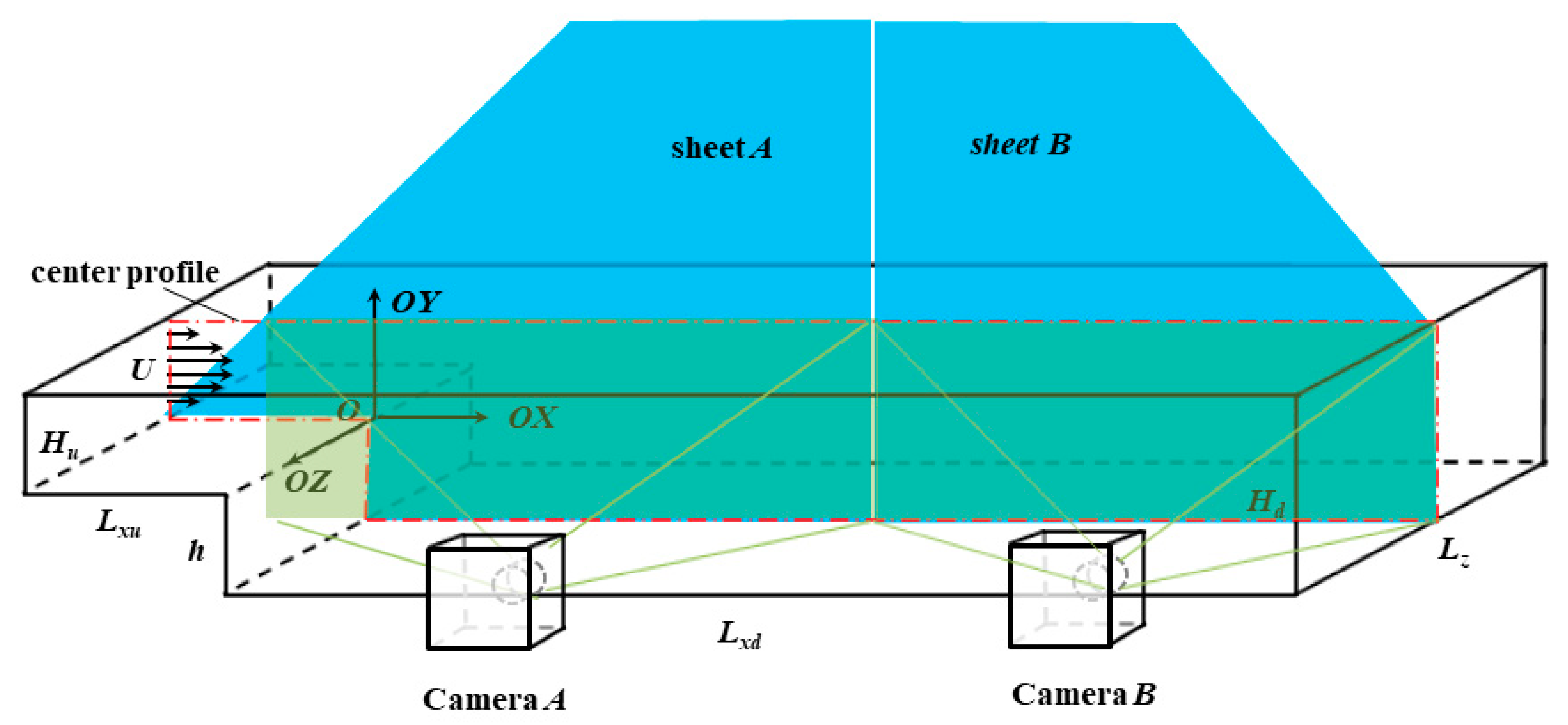
A water tunnel flow system with a BFS model was built (Figure 3) and some configuration parameters were listed in Table 1. A rectangular pressured tunnel was set horizontally (top wall slope, i = 0). It enlarges halfway and forms a vertical step at the bottom surface with h = 50 mm. The expansion ratio, Er = Hd/Hu, equals to 2, where Hd and Hu are respectively water depth upstream and downstream the step. The tunnel width was suggested to be no less than 10 h to keep the flow bidimensionality [16], therefore Ar = Lz/h = 10 was set. The channel lengths of upstream and downstream the step were Lxu = 44 h and Lxd = 50 h, respectively. Honeycomb tubes were set near the inlet of the channel to obtain fully developed turbulent flow before the step.
The flow tunnel was made of transparent PMMA (polymethyl-methacrylate) to provide a clear view for the PIV system. PIV was employed to measure the velocity fields at the central profile (Figure 3).
2.2. Measurement System
According to the previous literatures, Xr behind step was about (4.2~8.6) h when flow was fully turbulent, and it was even longer for a lower Reynold number [1,11,20,30]. To study the evolution process of the CVS, a global view of velocity fields with no less than 10 h (about 60 cm) behind the step was expected. A large-scale field of view was difficult to realize with high vector density and high precision. To obtain the global velocity field, some previous studies took pictures of different subareas and matched the time-averaged velocity fields spatially [14,29]. However, this was still unavailable for the global view of the instantaneous velocity fields with CVS’ evolution process. This study developed a synchronous PIV system, by which a doubled and effective view of the instantaneous velocity field was achieved (Figure 3, Sheets A and B).
The synchronous PIV system mainly consisted of laser module, image acquisition module, and control module. The laser module was a laser whose ray scanned to a light sheet optics with thickness of about 1 mm. The laser power energy was 3 W and the maximum scanning frequency reached to 40 Hz. The image acquisition module was made of a charge coupled device (CCD) camera with a resolution about 2560 pix × 2048 pix. Hollow sphere glass particles were seeded into the water with an average diameter of 15 μm. Two light sheets (A and B) and cameras (A and B) were synchronously controlled by a control module. This PIV system successfully made a global view of an instantaneous velocity field of approximate 12 h × 5 h with a resolution of 7.35 pix/mm. Interrogation area of 20 pix × 15 pix (2.722 mm × 2.042 mm) was used when computing velocity vectors. The measurement accuracy was within 1% of the maximum velocity.
2.3. Flow Conditions
The experiment was carried out with a constant water head for each case. The Reynolds number, Reh = Ubh/ν, was defined by the step height and the averaged velocity (Ub) located at 1 h upstream the step, and ν was the kinematic viscous coefficient of water at 20 °C.
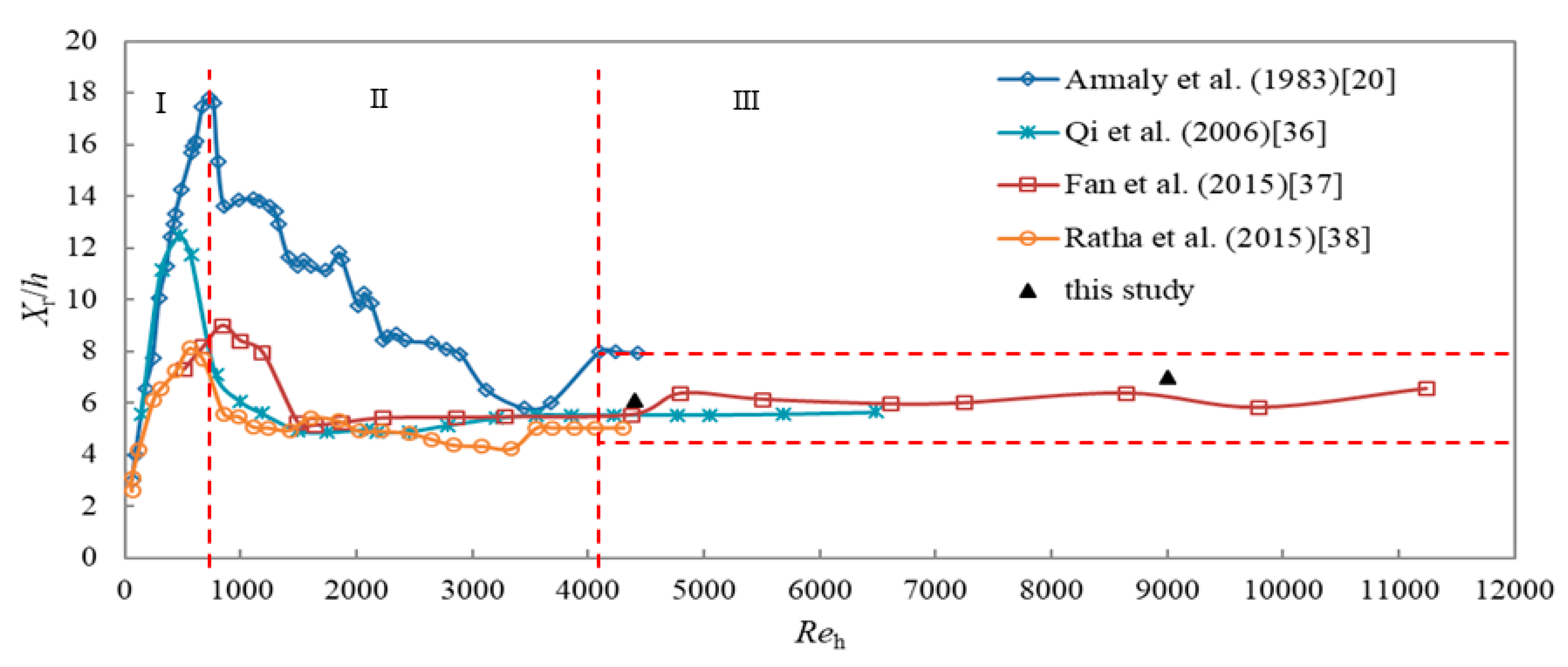
Figure 4 shows the relationship between Xr and Reh. Three typical flow regions were identified: the laminar flow (region I, Reh < 740), transition flow (region II, 740 < Reh < 4070), and turbulent flow (region III, Reh > 4070). A relative stable recirculation region with a constant Xr value (4.2~8.6 h) occurs in the turbulent flow (III) [1,20,36,37,38]. The flow structures in this flow region (III) were proposed to be stable, while the Xr values in another two flow patterns (I and II) were both changeable. Since most flow are with high Reynolds number in real applications, the turbulent flow region (III) were particularly favored here. For comparison, two cases with Reh = 4400 and Reh = 9000 were analyzed (Table 2). In addition, the good agreement of the data points in Figure 4 also verify the reliability of the measuring instrument.
3. Results and Discussions
3.1. Vortex Visualization and Definition
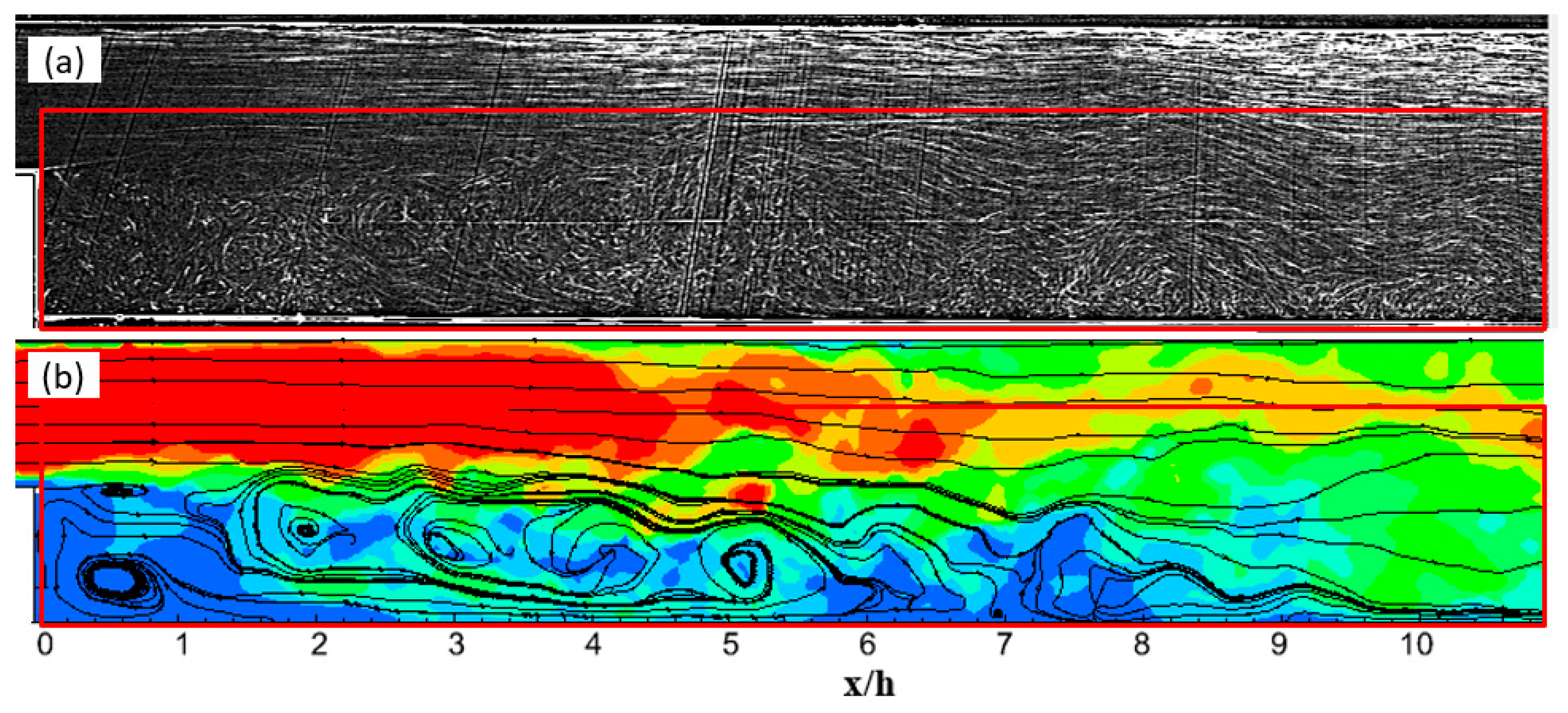
The vortex structures are visualized by the ghosting pictures of the inspired particles, and the pictures are also compared with the instantaneous streamlines (Figure 5). Comparison shows that the two figures present similar flow phenomena. The main flow diffuses and forms a recirculation region behind the step. The instantaneous flow is turbulent with the main flow interacting with the recirculation region.
Particularly, the streamlines show some spanwise and large-scale vortex structures behind the step. They are well organized in time and space. They successively roll up in the FSR, move downstream and approach to the reattachment zone, with maximum length scale of the same order with the step height. These vortex structures present mostly an elliptical shape from a side view particularly in the early developing stage, and then break down when approaching the reattachment zone. These flow phenomena are consistent with the visualization of Tani et al. (1961) in Figure 2a [22].
One may ask if these elliptical streamlines are vortices or not. Lugt (1979) [39] defined a vortex as “multitude of material particles rotating around a common center.” Robinson (1991) [40] further concluded that a vortex exists when instantaneous streamlines mapped onto a plane normal to the vortex core exhibit a roughly circular spiral pattern, when viewed from a reference frame moving with the center of the vortex core. These two definitions both propose two major features (“a common center” and “rotating”), and the later one further points to use streamlines to show a vortex. Although the concept of CVS has been proposed for centuries, its physical definition is still ambiguous. The vortex structures in the flow visualizations or by streamlines have the basic vortical features, particularly the streamlines show some elliptical patterns which rotates around a common center. Thus, they are consistent with the vortical definitions. Here, we define these vortex structures shown by streamlines to be the coherent vortex structures.
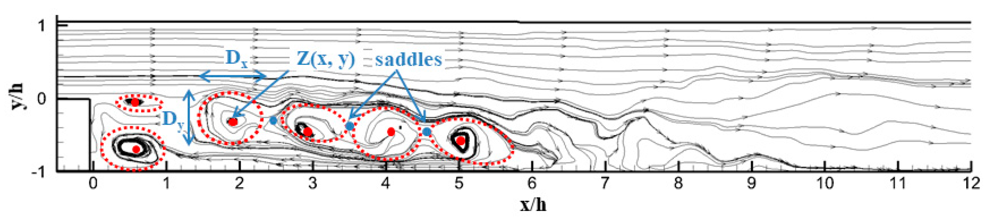
To quantitatively describe these CVS, some basic parameters such as the locations and patterns are defined (Figure 6). The common center of streamlines is regarded as the vortex core (Z(x, y)), representing location of a vortex. The typical shape is regarded close to an ellipse with streamwise diameter (Dx), and vertical diameter (Dy). Thus, Dx/Dy represents width to height ratio and D = 0.5 × (Dx + Dy) indicates the mean scale. Two CVS are separated by an equilibrium point, called the saddle point.
3.2. Vortex Motions with Developing Stages
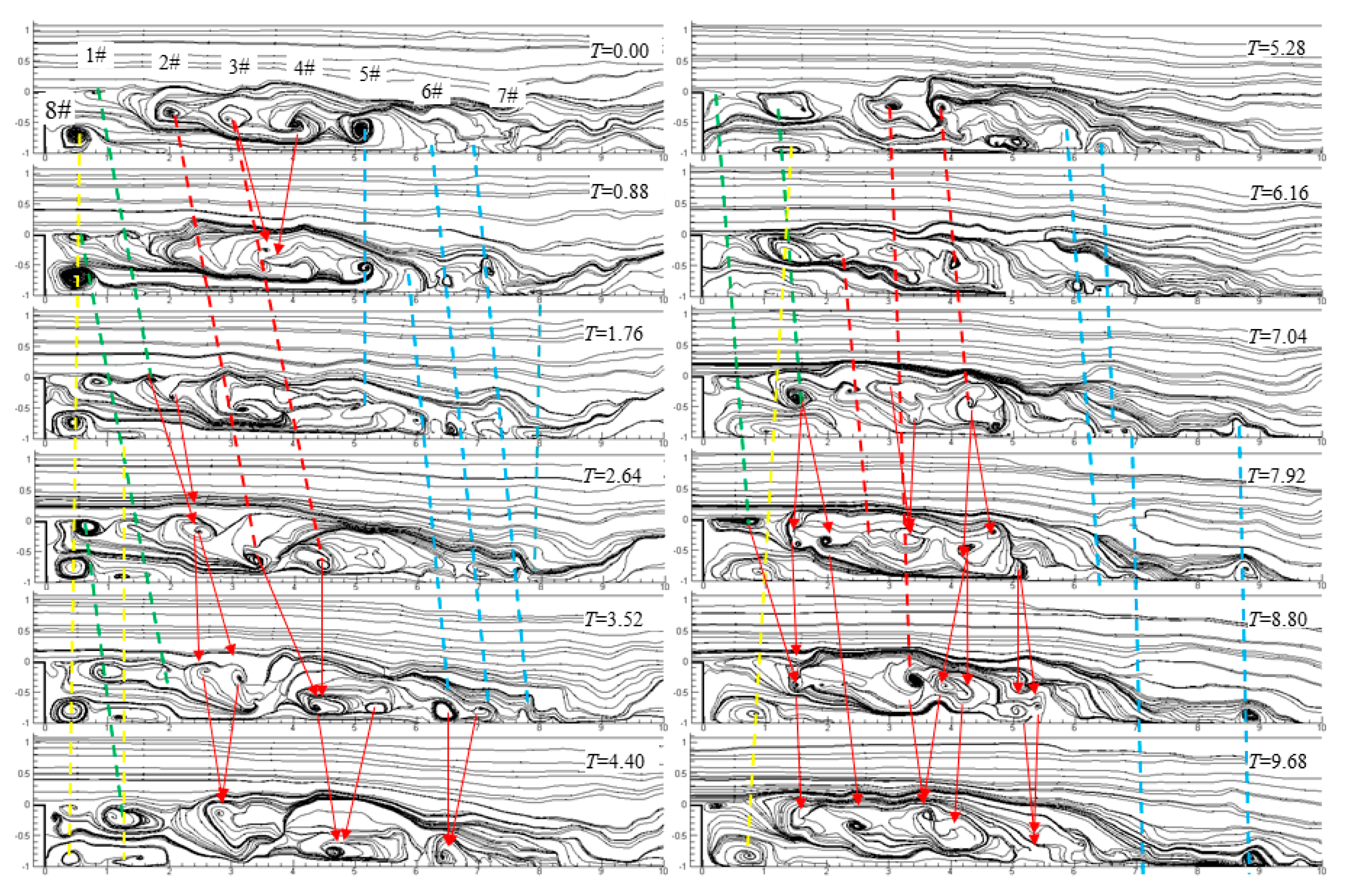
Figure 7 shows the spatial and temporal evolution process of the CVS in streamline pictures. Totally 12 instantaneous streamline pictures with an interval time of 0.5 s are compared (T = tUb/h = 0.00~9.68). These streamlines are generated with the corresponding velocity matrix by TECPLOT 2013.
In the first picture (T = 0.00), eight representative CVS (#1~#8) are indexed, which show various patterns and characteristics with flow structures (flow regions and developing stages see Figure 1). An analysis for these CVS’ features based on the flow structures divided is conducted here.
(1) Vortex #1 is located in the forming stage (the first stage, x = (0~2) h in FSR) just behind the step. Strong free shear layer is developing from the step corner with increasing thickness. Successive vortex structures generate and grow with similar size (diameter < 0.5 h) when travelling downstream (green lines). Finally, they are mixed by larger and fully developed ones at the end of this stage (x = (1~2) h). Their average speed toward downstream is about (0.3~0.6) Ub in this case.
(2) Vortex #2~#5 occur in the developing stage (the second stage, x = (2~5) h in FSR). The CVS are fully developed and energetic with larger length scales that close to h. Abundant amalgamation (pairing) and division events happen in this stage (red arrow lines). Because of the high mixing rate and flow unsteadiness, the turbulent intensity and shear stress reach a peak there [1,11,14]. This response may be a proof that the CVS is an important contributor for the Reynolds stress. Compared with the former stage, their travelling speeds reduce to approximately (0.05~0.3) Ub before attaching to the reattachment zone (red lines).
(3) Vortex #6~#7 appear in the shedding stage (the third stage, x = (5~8) h in the reattachment zone). Flow is strongly disturbed by the bottom wall in this stage. The streamlines are twisted sometimes when approaching to the wall. This may be induced by the enhancement of the three-dimensional characteristics. The CVS slow down and mostly attach on the bottom wall (blue lines), and sometimes they vanish there. Beyond R, some streamlines begin to roll up and generate some new vortex structures in a relatively smaller length scale and weaker rotating intensity. These vortex structures usually keep for a short time.
(4) Vortex #8 is usually found in the corner region (x = (0~2) h in CR). It is induced by the recirculation, where the backflow separates from bottom wall and induces a counter-clockwise vortex [14,20,27,35]. The temporal evolution shows that the separation streamline is usually generated at the separated point of the backflow leaving the wall. The diameter of this vortex is about 0.5 h [11]. This vortex has a much weak rotating intensity. And it travels upstream at the speed of about 0.1 Ub in this case (yellow lines, Reh = 4400).
There are totally dozens of CVS in each streamline picture. The evolution shows a life process of forming, developing, shedding, and redeveloping when travelling downstream. Their characteristics such as size, rotation direction and intensity, and evolution behaviors vary with the flow regions and developing stages. In particular, amalgamation (pairing) and division behaviors often occur in the second developing stage.
3.3. Vortex Trajectory and Evolution
The life process of the CVS is also reflected in the temporal evolution of an individual vortex structure. The blue line tracks the trajectory of a typical vortex center and other color lines show some break up and amalgamation (Figure 8). In this figure, the blue diamond point means the vortex center and the arrows show its moving direction. It starts nearby the step corner, and then travels toward the reattachment zone. It initially wanders in the strong shear layer, forming a relatively narrow path in the first stage (forming stage, 0~2 h). When arriving to the end of this stage, the center “jump” at about x = 1.5 h, which can be explained by the amalgamation (merged by the vortex in later stage) shown in Figure 7. Then the vortex lingers and fluctuates particularly around x = 2.2 h and x = 3.4 h in the developing stage, where frequent amalgamation and division events occur there. The branches lines with other colors indicate vortex structures breaking up from the original one. When travelling to the end of this stage (x = 4~5 h), the original vortex could not be found in the streamline pictures.
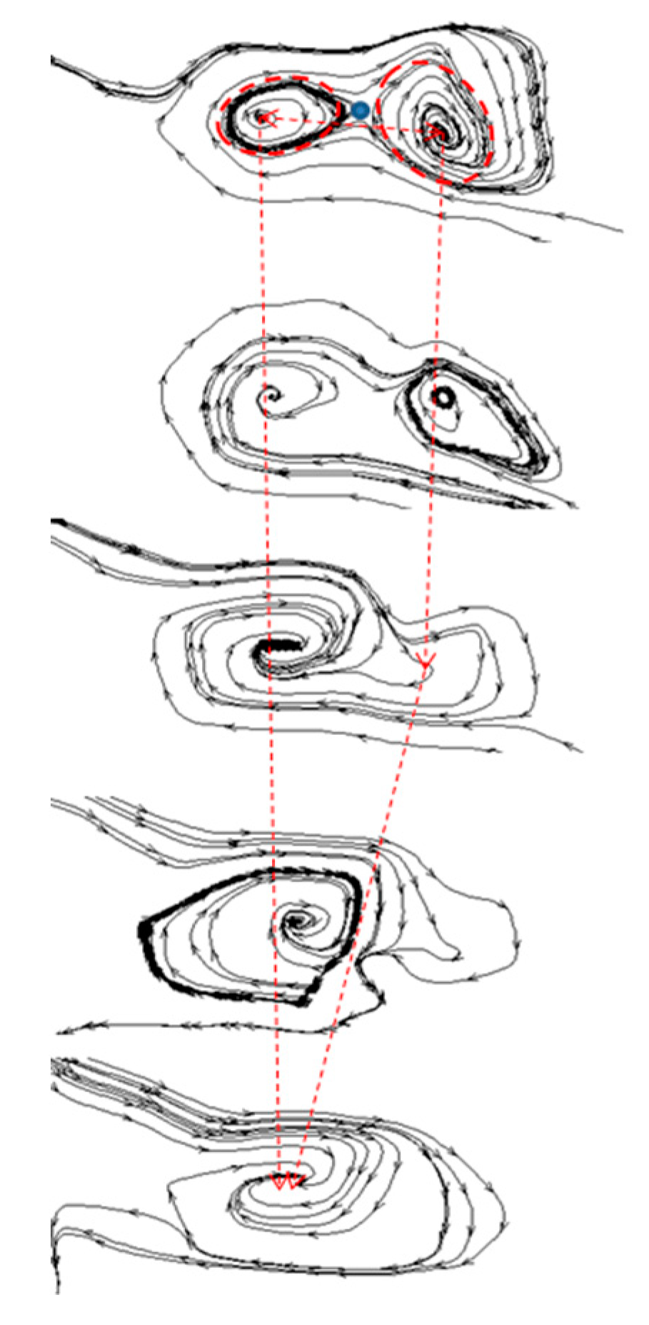
To further investigate the evolution events, a typical pairing process of two CVS is analyzed (Figure 9). To our knowledge, there is no experimental analysis for this process. A critical distance, λc, between two vortex patches was numerically studied by the contour dynamics method, and a distance parameter, λ, was defined when considering two scheduled circular vortex patches with the same diameters and shown by certain vorticity contour [41,42]:
where L is the distance between the two vortex patches, and r is the radius of each vortex patch.
λ = L/r (L > 2 r)
When λ > λc, these two vortex patches rotate and change in shape, and their shape is close to a tear drop with the decrease of λ. When λ < λc (λc = 3.5), these two vortex patches start to interact with each other. With the decrease of λ, they will get tangled up and finally they merge together.
In this experimental study, a similar parameter λ’ is defined between two vortex structures with equivalent radiuses of r1 and r2, respectively (Equation (2)). A critical value is also expected when the CVS start to pair. It should be pointed out that these CVS are defined by streamlines instead of vorticity contours, and they are mostly elliptical but not circular in shape.
where L’ is the distance between two vortex centers, and r1 and r2 are of the equivalent radiuses of two CVS, respectively.
λ’ = 2 L’/(r1 + r2) (2 L’ > r1 + r2)
As is shown in Figure 9, two CVS keep independent initially when they stay at a sufficiently far distance. As they are getting closer, they change in shape and start to interact with each other and finally come to an amalgamation when their distance is less than the critical value (λ’ < λc). This indicates that critical distance still exists in current CVS. From the point view of the direction of the streamlines, these two CVS have an opposite streamline direction, one converges to the center (right) and another originates from the center (left). The former one is usually stable, while the other one is unstable. They finally merge into a stable one (streamlines converge to the vortex center).
3.4. Vortex Center and Diameter Distributions
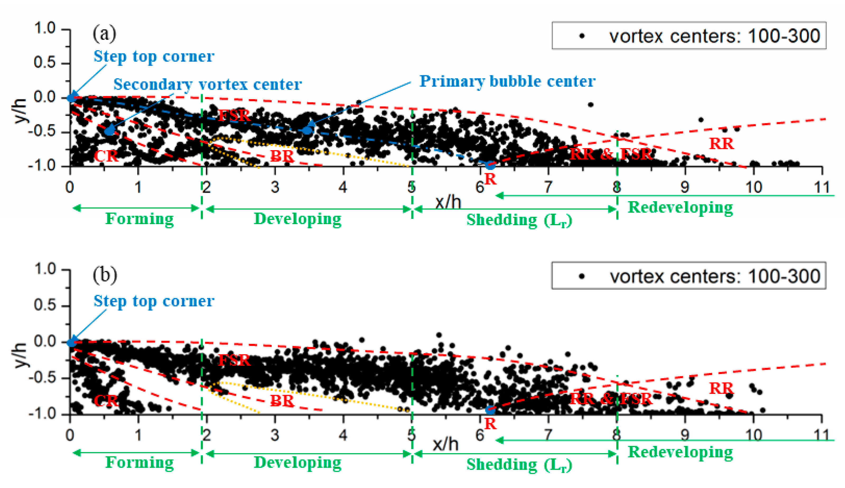
Temporal evolution of the specific vortex structure is particularly disclosed above, their features of spatial distribution and length scales are to discuss here. Totally more than 2000 CVS were extracted from 201 instantaneous streamline pictures (picture no. 100–300), and the distributions of vortex centers (Z(x, y)) and diameters parameters (Dx, Dy, D, Dx/Dy) were statistically analyzed (Figure 10 and Figure 11).
Figure 10 shows the distribution of the vortex centers with Reh = 4400 and 9000 separately. The distribution seem to be regular, that fit well with the divided flow regions and developing stages (Figure 1). The vortex centers mainly distribute in the FSR, CR, and RR. In other words, these CVS are directly and closely related to the flow separation and reattachment characteristics. And they present specific features in different regions, going through the process of forming, developing, shedding, and redeveloping when travelling downstream. This statistical distribution also supports well the above discussion on vortex center trajectory and vortex evolution. With increase of Reh from 4400 to 9000, the distribution of vortex centers is almost unchanged in space. It provides a good explanation for the various features with the specific flow structures.
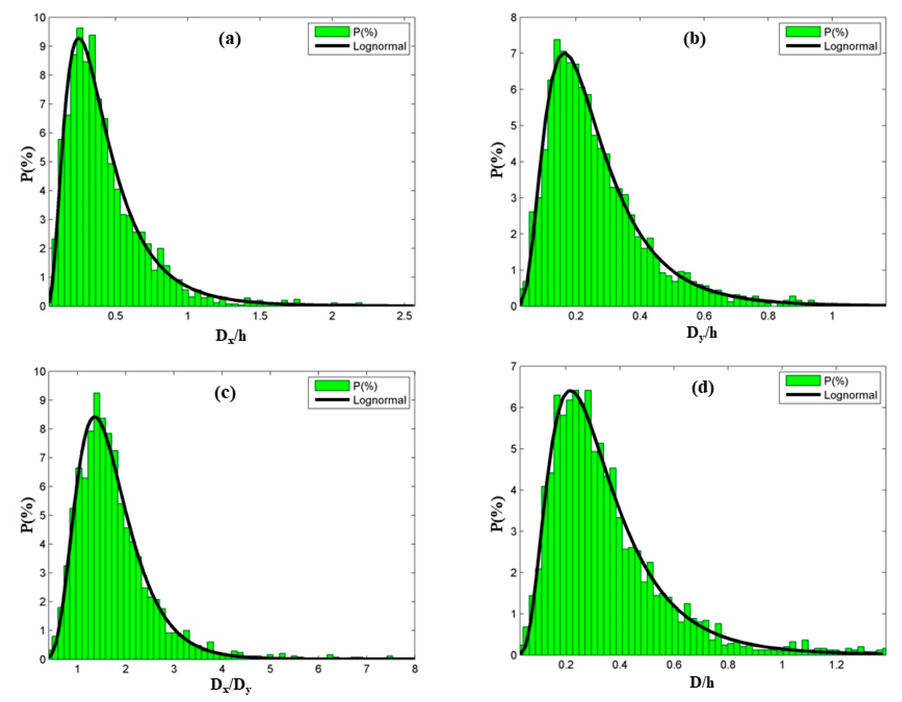
Besides the vortex center, the distribution of parameters Dx, Dy, Dx/Dy, and D are also well organized. Over 2000 vortex structures are analyzed. Figure 11 shows that four parameters (Dx, Dy, Dx/Dy, and D) all obey to the lognormal distribution. In other words, their logarithms follow a normal distribution. We know that lognormal distributions are positively skewed with long right tails because of low mean values and high variances in the random variables. The mean value (exp(μ)) and standard deviation (σ) were used to evaluate the length scale for the CVS, and also compare the influences of Reynolds number (Reh = 4400 and 9000) and geometric model (BFS and turbulent boundary layer, TBL). The mean value (exp(μ)) and standard deviation (σ) were obtained by data fitting and are compared in Table 3.
With the increase of Reh from 4400 to 9000, these four variables change with different trends. The streamwise diameter (Dx/h) decreases slightly from 0.36 to 0.32, while the vertical diameter (Dy/h) increases from 0.22 to 0.24. As a result, the width to height ratio (Dx/Dy) reduces from 1.51 to 1.40. This means that the long axis of the ellipse becomes shorter and the short axis grows, making the shape more circular with increasing of Reh. However, the mean diameter (D/h) keeps a relative stable value around 0.28~0.29 for current experimental conditions. The standard deviation σ of variables (Dx/h, Dy/h, and D/h) all increase with increase of Reh, while that of Dx/Dy has almost no response to Reh. With the increase of Reh, previous study showed that the shear intensity behind the step increases, and flow turbulence or unsteadiness is enhanced [20]. This will contribute to the vortex mixing and accelerate vortex evolution. We can understand that the streamwise diameter (Dx) is generally greater than the vertical diameter (Dy) as the streamwise shear direction and vertical wall constraints.
An experimental study of a turbulent boundary layer (TBL) on the distribution for vortex length scales was reported by Wang (2009) [43]. Different to the BFS configuration, there is a free water surface and no disturbance of step in the TBL model, yet the Reynold number, Reb = UbR/ν = 4677 (R is hydraulic radius), is the same order with this study. In comparison, the CVS are more circular because of the vortical pattern Dx/Dy = 1.40–1.51 in the BFS flow is smaller than Dx/Dy = 2.18 in TBL flow. This may be explained by the different features of their shear layers, where the CVS are initially formed. The shear intensity is particularly strong near the bottom wall with a uniform mean velocity direction in TBL. While shear layer in BFS initially generates and develops from the step with a recirculation below. The extra recirculation and less impact of the wall in BFS flow both contribute to the more circular vortical shape. As for the standard deviation (σ), the BFS flow shows a smaller value than that of TBL flow. This means a more concentrated vortex scale distribution in BFS flow.
4. Conclusions and Recommendations
Velocity measurements and CVS investigation for the experiments at a BFS water flow with Reh = 4400 and 9000 were reported. From a viewpoint of CVS defined in the streamline pictures, the vortical spatio-temporal coherences were verified and quantitatively studied. The following conclusions may be drawn:
(1) A synchronized PIV system is necessary for the measurement of a wider range of velocity fields with sufficiently high resolution to study the global evolution process of CVS.
(2) CVS are proved to exist in the separation and reattachment process of BFS flow. They are well organized in the recirculation regions with forming, developing, shedding, and redeveloping in the shear layer. Flow structures with various local characteristics are disclosed and explained by the motions and evolutions of CVS.
(3) The spatial distribution of CVS is almost unaffected by the Reynolds number when flow is fully turbulent. The CVS are particularly active at the developing stage with frequent pairings and divisions, which contribute to the high turbulent intensity and shear stress. And the shedding of CVS can explain the rapid decrease of the Reynolds stress at the reattachment zone.
(4) Statistics show the streamwise (Dx/h), vertical (Dy/h), and mean (D/h) diameters, and width to height ratio (Dx/Dy) of the CVS all obey to the lognormal distribution. The mean diameter (D/h) is about 0.28~0.29 for a BFS flow with Reh = 4400 and 9000. Compared with the flow in a turbulent boundary layer, they have the same order of vortex length scale, while the shape of CVS in BFS is more circular. A critical distance is supposed to exist between two CVS.
Concept of CVS has been put forward for more than half a century and it is proved to play a significant role particularly in the separated flows. With the development of measurement techniques and numerical simulations, more quantitative information should be used to verify the previous hypothesis and suggestions. The quantitative vortex length scales measured in the experiments may help to choose the grid scale in certain simulations considering the large-scale vortex structures (such as the Large Eddy Simulation). In terms of the local energy dissipation at the enlarged step, the significant impact of the CVS cannot be ignored.
Author Contributions
F.W. and S.W. conceived and designed the experiment; F.W. and A.G. performed the experiment and analyzed the data and wrote the manuscript. S.Z., A.G., J.D., and Q.L. contributed to scientific advising and provided a substantial input to improve the paper.
Funding
This research is funded by the National Natural Science Foundation of China (Grant No. 51909169), the Science and Technology Support Program of Jiangsu Province (Grant No. SBK2019042181), and the financial support from Nanjing Hydraulic Research Institute (NHRI) (Grant No. Y119005). The authors gratefully acknowledge these financial supports.
Acknowledgments
The authors would also like to thank Corporation Hawksoft for their assistances in the laboratory measurements.
Conflicts of Interest
The authors declare no conflict of interest.
References
- Eaton, J.K.; Johnston, J.P. A review of research on subsonic turbulent flow reattachment. AIAA J. 1981, 19, 1093–1100. [Google Scholar] [CrossRef]
- Vogel, J.C.; Eaton, J.K.; Adams, E.W. Combined heat transfer and fluid dynamic measurements behind a backward-facing step. Am. Soc. Mech. Eng. 1985, 107, 922–929. [Google Scholar]
- Jacob, M.C.; Guerrand, S.; Juvé, D.; Guerrand, S. Experimental study of sound generated by backward-facing steps under wall jet. AIAA J. 2001, 39, 1254–1260. [Google Scholar] [CrossRef]
- Hu, R.Y.; Wang, L.; Fu, S. Review of backward-facing step flow and separation reduction. Sci. Sin. Phys. Mech. Astro. 2015, 45, 124704. (In Chinese) [Google Scholar]
- Chen, L.; Asai, K.; Nonomura, T.; Xi, G.; Liu, T. A review of backward-facing step (BFS) flow mechanisms, heat transfer and control. Therm. Sci. Eng. Prog. 2018, 6, 194–216. [Google Scholar] [CrossRef]
- Chun, K.B.; Sung, H.J. Visualization of a locally-forced separated flow over a backward-facing step. Exp. Fluids 1998, 25, 133–142. [Google Scholar] [CrossRef]
- Chen, L.; Zhang, X.R.; Okajima, J.; Maruyama, S. Thermal relaxation and critical instability of near-critical fluid microchannel flow. Phys. Rev. E 2013, 87, 043016. [Google Scholar] [CrossRef]
- Baigmohammadi, M.; Tabejamaat, S.; Farsiani, Y. Experimental study of the effects of geometrical parameters, Reynolds number, and equivalence ratio on ethaneoxygen premixed flame dynamics in non-adiabatic cylindrical meso-scale reactors with the backward facing step. Chem. Eng. Sci. 2015, 132, 215–233. [Google Scholar] [CrossRef]
- Shahi, M.; Kok, J.B.W.; Pozarlik, A. On characteristics of a non-reacting and a reacting turbulent flow over a backward facing step (BFS). Int. Commun. Heat Mass Transf. 2015, 61, 16–25. [Google Scholar] [CrossRef]
- Dodaro, G.; Tafarojnoruz, A.; Sciortino, G.; Adduce, C. Modified Einstein sediment transport method to simulate the local scour evolution downstream of a rigid bed. J. Hydraul. Eng. 2016, 142, 04016041. [Google Scholar] [CrossRef]
- Wang, F.F.; Wu, S.Q.; Huang, B. Flow structure and unsteady fluctuation for separation over a two-dimensional backward-facing step. J. Hydrodyn. 2019. [Google Scholar] [CrossRef]
- Roos, F.W.; Kegelman, J.T. Control of coherent structures in reattaching laminar and turbulent shear layers. Aiaa J. 1986, 24, 1956–1963. [Google Scholar] [CrossRef]
- Wee, D.; Yi, T.; Annaswamy, A.; Ghoniem, A.F. Self-sustained oscillations and vortex shedding in backward-facing step flows: Simulation and linear instability analysis. Phys. Fluids 2004, 16, 3361–3373. [Google Scholar] [CrossRef]
- Kostas, J.; Soria, J.; Chong, M. Particle image velocimetry measurements of a backward-facing step flow. Exp. Fluids 2002, 33, 838–853. [Google Scholar] [CrossRef]
- Hudy, L.M.; Naguib, A.; Humphreys, W.M. Stochastic estimation of a separated-flow field using wall-pressure-array measurements. Phys. Fluids 2007, 19, 1093. [Google Scholar] [CrossRef]
- Bradshaw, P.; Wong, F.Y.F. The reattachment and relaxation of a turbulent shear layer. J. Fluid Mech. 1972, 52, 113–135. [Google Scholar] [CrossRef]
- Nadge, P.M.; Govardhan, R.N. High Reynolds number flow over a backward-facing step: Structure of the mean separation bubble. Exp. Fluids 2014, 55, 1657–1678. [Google Scholar] [CrossRef]
- Calomino, F.; Tafarojnoruz, A.; De Marchis, M.; Gaudio, R. Experimental and numerical study on the flow field and friction factor in a pressurized corrugated pipe. J. Hydraul. Eng. 2015, 141, 04015027. [Google Scholar] [CrossRef]
- Calomino, F.; Alfonsi, G.; Gaudio, R.; D’Ippolito, A.; Lauria, A.; Tafarojnoruz, A.; Artese, S. Experimental and numerical study of free-surface flows in a corrugated pipe. Water 2018, 10, 638. [Google Scholar] [CrossRef] [Green Version]
- Armaly, B.F.; Durst, F.J.; Pereira, J.C.F.; Schönung, B. Experimental and theoretical investigation of backward-facing step flow. J. Fluid Mech. 1983, 127, 473–496. [Google Scholar] [CrossRef]
- Simpson, R.L. Review—A review of some phenomena in turbulent flow separation. J. Fluids Eng. 1981, 103, 520–533. [Google Scholar] [CrossRef]
- Tani, I.; Iuchi, M.; Komoda, H. Experimental Investigation of Flow Separation Associated with a Step or a Groove; Aeronautical Research Institute, University of Tokyo: Tokyo, Japan, 1961; p. 364. [Google Scholar]
- McGuinness, M. Flow with a Separation Bubble—Steady and Unsteady Aspects. Ph.D. Thesis, Cambridge Univ., Cambridge, UK, 1978. [Google Scholar]
- Chandrsuda, C. A Reattaching Turbulent Shear Layer in Incompressible Flow. Ph.D. Thesis, Dept. of Aeronautics, Imperial College of Science and Technology, London, UK, 1975. [Google Scholar]
- Kim, J.; Kline, S.J.; Johnston, J.P. Investigation of Separation and Reattachment of a Turbulent Shear Layer: Flow over a Backward-Facing Step; Thermosciences Div., Dept. of Mechanical Engineering, Stanford Univ., Rept. MD-37: Stanford, CA, USA, 1978. [Google Scholar]
- Etheridge, D.W.; Kemp, P.H. Measurements of turbulent flow downstream of a rearward-facing step. J. Fluid Mech. Digit. Arch. 1978, 86, 22. [Google Scholar] [CrossRef]
- Lian, Q.X. An experimental investigation of the coherent structure of the flow behind a backward facing step. Acta Mech. Sin. 1993, 9, 129–133. (In Chinese) [Google Scholar]
- Stevenson, W.H.; Thompson, H.D.; Craig, R.R. Laser velocimeter measurements in highly turbulent recirculating flows. J. Fluids Eng. 1984, 106, 173–180. [Google Scholar] [CrossRef]
- Scarano, F.; Benocci, C.; Riethmuller, M.L. Pattern recognition analysis of the turbulent flow past a backward facing step. Phys. Fluids 1999, 11, 3808–3818. [Google Scholar] [CrossRef]
- Ma, X.; Geisler, R.; Schroder, A. Experimental investigation of separated shear flow under subharmonic perturbations over a backward-facing step. Flow Turbul. Combust. 2017, 99, 71–91. [Google Scholar] [CrossRef]
- Driver, D.M.; Seegmiller, H.L.; Marvin, J.G. Time-dependent behavior of a reattaching shear layer. AIAA J. 1987, 25, 914–919. [Google Scholar] [CrossRef]
- Le, H.; Moin, P.; Kim, J. Direct numerical simulation of turbulent flow over a backward-facing step. J. Fluid Mech. 1997, 330, 349–374. [Google Scholar] [CrossRef] [Green Version]
- Aider, J.; Danet, A.; Lesieur, M. Large-eddy simulation applied to study the influence of upstream conditions on the time-dependant and averaged characteristics of a backward-facing step flow. J. Turbul. 2007, 8, 1–30. [Google Scholar] [CrossRef]
- Kopera, M.A.; Kerr, R.M.; Blackburn, H.M.; Barkley, D. Direct numerical simulation of turbulent flow over a backward-facing step. J. Fluid Mech. 2014. under publication. [Google Scholar]
- Hu, R.Y.; Wang, L.; Fu, S. Investigation of the coherent structures in flow behind a backward-facing step. Int. J. Numer. Methods Heat Fluid Flow 2016, 26, 1050–1068. [Google Scholar] [CrossRef]
- Qi, E.R.; Huang, M.H.; Li, W.; Zhang, X. An experimental study on the 2D time average flow over a backward facing step via PIV. J. Exp. Mech. 2006, 21, 225–232. (In Chinese) [Google Scholar]
- Fan, X.J.; Wu, S.Q.; Zhou, H.; Xiao, X.; Wang, Y. Investigation on the Characteristics of Water Flow over a Backward Facing Step under High Reynolds Number with Particle Image Velocimetry. In Proceedings of the International Conference on Industrial Technology and Management Science, Tianjin, China, 27–28 March 2015. [Google Scholar]
- Ratha, D.; Sarkar, A. Analysis of flow over backward facing step with transition. Front. Struct. Civ. Eng. 2015, 9, 71–81. [Google Scholar] [CrossRef]
- Lugt, H.J.; Gollub, J.P. Vortex Flow in Nature and Technology; Wiley: Hoboken, NJ, USA, 1972. [Google Scholar]
- Robinson, S.K. Coherent motions in the turbulent boundary layer. Annu. Rev. Fluid Mech. 1991, 23, 601–639. [Google Scholar] [CrossRef]
- Deem, G.S.; Zabusky, N.J. Stationary “V-States,” interactions, recurrence, and breaking. Phys. Rev. Lett. 1978, 41, 518. [Google Scholar] [CrossRef]
- Wu, J.Z.; Ma, H.Y.; Zhou, M.D. Introduction to Vorticity and Vortex Dynamics; Advanced Education Press: Beijing, China, 1993; pp. 463–466. [Google Scholar]
- Wang, L. Experimental Study on Coherent Structure in Open-Channel Flow. Ph.D. Thesis, Tsinghua University, Beijing, China, 2009. (In Chinese). [Google Scholar]
Figure 1.
Simplified representation of a two-dimensional backward-facing step (BFS) flow: (FSR: free shear region; CR: corner region; RR: redeveloping region; R: mean reattachment point).
Figure 1.
Simplified representation of a two-dimensional backward-facing step (BFS) flow: (FSR: free shear region; CR: corner region; RR: redeveloping region; R: mean reattachment point).

Figure 2.
Visualizations of BFS flow: (a) Tani et al. (1961) [22]; (b) Chun et al. (1998), without excitation [6]; (c) Chun et al. (1998), with excitation [6]; (d) Kostas et al. (2002) [14].

Figure 3.
Schematic of the test section arrangements with a synchronous particle image velocimetry (PIV) system.
Figure 3.
Schematic of the test section arrangements with a synchronous particle image velocimetry (PIV) system.

Figure 4.
The reattachment length (Xr) vs. Reynolds number (Reh).

Figure 5.
Coherent vortex structures (CVS) in the instantaneous flow: (a) visualization, (b) streamlines with velocity contours.
Figure 5.
Coherent vortex structures (CVS) in the instantaneous flow: (a) visualization, (b) streamlines with velocity contours.

Figure 6.
Parameter definition for the CVS (Dx—streamwise diameter, Dy—vertical diameter, Z(x, y)—vortex center, blue point—saddle point).
Figure 6.
Parameter definition for the CVS (Dx—streamwise diameter, Dy—vertical diameter, Z(x, y)—vortex center, blue point—saddle point).

Figure 7.
Motions and evolutions of the CVS with Reh = 4400 (Dash lines with green, red, blue and yellow represent vortex trajectory in different developing stages; Arrow lines represent the amalgamation and division behaviors; T = 0.00~9.68).
Figure 7.
Motions and evolutions of the CVS with Reh = 4400 (Dash lines with green, red, blue and yellow represent vortex trajectory in different developing stages; Arrow lines represent the amalgamation and division behaviors; T = 0.00~9.68).

Figure 8.
Trajectory and evolution of vortex centers (Reh = 4400).

Figure 9.
A vortex pairing process.

Figure 10.
Distribution of the CVS with different Reh: (a) Reh = 4400 [11] and (b) Reh = 9000; (FSR: free shear layer region, CR: corner region; BR: backflow region; RR: redeveloping region; R: reattachment point; Lr: length of reattachment zone).
Figure 10.
Distribution of the CVS with different Reh: (a) Reh = 4400 [11] and (b) Reh = 9000; (FSR: free shear layer region, CR: corner region; BR: backflow region; RR: redeveloping region; R: reattachment point; Lr: length of reattachment zone).

Figure 11.
Distribution of length scale parameters (Reh = 4400): (a) Dx; (b) Dy; (c) Dx/Dy; (d) D.


Table 1.
Configuration parameters of the BFS model.
| Parameters | Values | Units |
|---|---|---|
| h | 50 | mm |
| Lxu | 2220 | mm |
| Lxd | 2500 | mm |
| Hu | 50 | mm |
| Hd | 100 | mm |
| Lz | 500 | mm |
| i | 0 | ° |
| Er | 2:1 | - |
| Ar | 10:1 | - |
Table 2.
Flow conditions in the experiment.
| h (cm) | Ub (m/s) | Er | Ar | Reh | Xr/h |
|---|---|---|---|---|---|
| 5 | 0.088 | 2:1 | 10 | 4400 | 6.1 |
| 5 | 0.182 | 2:1 | 10 | 9000 | 7.0 |
Table 3.
Comparison of the length scale parameters (BFS and TBL).
| Literature | Configuration | Parameter | μ | Exp (μ) | σ |
|---|---|---|---|---|---|
| This study | BFS Reh = 4400 | Dx/h | −1.03 | 0.36 | 0.61 |
| Dy/h | −1.49 | 0.22 | 0.56 | ||
| Dx/Dy | 0.41 | 1.51 | 0.38 | ||
| D/h | −1.22 | 0.29 | 0.56 | ||
| BFS Reh = 9000 | Dx/h | −1.13 | 0.32 | 0.70 | |
| Dy/h | −1.43 | 0.24 | 0.68 | ||
| Dx/Dy | 0.33 | 1.40 | 0.37 | ||
| D/h | −1.26 | 0.28 | 0.68 | ||
| Wang (2009) [43] | TBL Reb = 4677 | Dx/hw | −1.37 | 0.25 | 0.69 |
| Dy/hw | −2.15 | 0.12 | 0.73 | ||
| Dx/Dy | 0.78 | 2.18 | 0.64 |
© 2019 by the authors. Licensee MDPI, Basel, Switzerland. This article is an open access article distributed under the terms and conditions of the Creative Commons Attribution (CC BY) license (http://creativecommons.org/licenses/by/4.0/).
Share and Cite
MDPI and ACS Style
Wang, F.; Gao, A.; Wu, S.; Zhu, S.; Dai, J.; Liao, Q. Experimental Investigation of Coherent Vortex Structures in a Backward-Facing Step Flow. Water 2019, 11, 2629. https://doi.org/10.3390/w11122629
AMA Style
Wang F, Gao A, Wu S, Zhu S, Dai J, Liao Q. Experimental Investigation of Coherent Vortex Structures in a Backward-Facing Step Flow. Water. 2019; 11(12):2629. https://doi.org/10.3390/w11122629
Chicago/Turabian StyleWang, Fangfang, Ang Gao, Shiqiang Wu, Senlin Zhu, Jiangyu Dai, and Qian Liao. 2019. "Experimental Investigation of Coherent Vortex Structures in a Backward-Facing Step Flow" Water 11, no. 12: 2629. https://doi.org/10.3390/w11122629
Note that from the first issue of 2016, this journal uses article numbers instead of page numbers. See further details here.