Investigation of the Sloshing Behavior Due to Seismic Excitations Considering Two-Way Coupling of the Fluid and the Structure


Department of Civil Engineering, Hydraulics Laboratory, Abdullah Gül University, Kayseri 38080, Turkey
Water 2019, 11(12), 2664; https://doi.org/10.3390/w11122664
Submission received: 5 November 2019
/
Revised: 3 December 2019
/
Accepted: 15 December 2019
/
Published: 17 December 2019
(This article belongs to the Section Hydraulics and Hydrodynamics)
Abstract
:Sloshing behavior due to near-fault type and earthquake excitations of a fluid in a tank having a highly deformable elastic structure in the middle was investigated experimentally and numerically in this paper. In the numerical model, fluid was simulated with smoothed particle hydrodynamics (SPH) and structure was simulated with the finite element method (FEM). The coupling was satisfied with contact mechanics. The δ-SPH scheme was adapted to lower the numerical oscillations. The proposed fluid-structure interaction (FSI) method can simulate the violent fluid-structure interaction problem successfully. The effects of near-fault type and earthquake excitations on free-surfaces of fluid and the elastic structure are presented.
1. Introduction
Sloshing, a highly nonlinear free-surface movement of fluid in partially filled tanks, is an important subject in fluid-structure interaction (FSI) problems. Violent sloshing occurs in partially filled tanks during earthquakes can cause dynamic loads on the tank structure. To prevent structural damage, a proper prediction of forces due to sloshing is critical.
Sloshing is generally affected by the geometry of the tank, the frequency and the amplitude of the movement, the amount of the liquid on the tank and the properties of the liquid. Experimental and numerical studies have been conducted to investigate the effect of the dimensions and the elasticity of the base of the tank and the frequency of the fluid-tank system on the sloshing under harmonic excitations [1,2,3,4,5,6,7,8,9,10]. Seakeeping problems by considering sloshing in tanks were investigated numerically with smoothed particle hydrodynamics (SPH)-finite element method (FEM) coupling [11]. A particle-based FSI solver was proposed to solve sloshing flows in roller tanks with elastic baffles [12]. Researchers have studied sloshing due to earthquake excitation experimentally and numerically [9,13,14,15,16,17]. There are more recent studies investigating sloshing due to seismic excitation that consider the effect of the interaction between the fluid and the structure [18,19,20].
In the present study, sloshing due to seismic excitation was investigated both experimentally and numerically. Real earthquake data was applied to a tank that had an elastic buffer in the middle. Various numerical models to couple fluid-structure interaction problems, such as MPS-FEM coupling [21] or immersed boundary methods combined with volume of fluid or level-set approaches [22,23,24], have been proposed in the literature [25]. In the present numerical model, smoothed particle hydrodynamics was coupled with the finite element method, and the coupling was satisfied with contact mechanics [26,27]. SPH, a Lagrangian and mesh-free method, was originally developed to simulate astrophysical problems [28,29]. SPH has successfully been applied to different scientific areas including fluid, soil and structural mechanics, impact problems etc. [30,31,32]. Recently, SPH was coupled with FEM to solve FSI problems. The first study coupling SPH and FEM was conducted to couple the interaction between two structures [33]. Two bars were impacted and SPH particles were treated as the nodes of the finite element. The coupling was satisfied with a master-slave algorithm, in which if an SPH particle assigned as a slave node enters the structural domain assigned as master node, this SPH particle is expelled from structural domain by conserving linear and angular momentum. In addition, the velocity components perpendicular to the surface were assumed to be the same [34,35]. The biggest disadvantage of a master-slave algorithm is the necessity of determining the master and slave surfaces, which increases the computational time. In one study [36], a contact algorithm allowing frictionless sliding between SPH particles and finite element was proposed. In this algorithm, finite element nodes were treated as SPH particles and a particle to particle contact approach was applied. Contact surface did not need to be defined. A continuous blending method was adapted to satisfy the contact between fluid and structure [37]. In the method, there were three regions. One region had only FE elements, the other region had only SPH particles. In the third region, both SPH particles and FE nodes were located. This region was called the transition region and the continuous blending method, originally developed for the coupling of moving least square and FEM, was applied. The shape function used for the continuous blending method is hard to get and computational cost is high [38]. Similarly, by adding FE nodes to the SPH neighbor list, SPH-FEM was coupled and contact force was calculated from the SPH particle to particle contact algorithm [38]. Contact occurs when the distance between an FE node and an SPH particle is less than two times the smoothing length; this is not similar to the reality. To lower the computational time of SPH-FEM, a searching algorithm was proposed [39]. In a more recent study, a weak coupling strategy, in which both SPH and FE solvers were treated as black boxes and a coupling program was used to exchange fluid pressures and nodal positions, was adapted [40]. Although the implementation is easy, there is no control over FE solver, which may be considered to be a disadvantage. A ghost particle method was proposed to complete the kernel and satisfy the first order consistency near the boundaries in SPH-FEM [41]. Since ghost particles were defined at every time step, the computational cost is relatively high.
The aim of the present study is to investigate sloshing due to the seismic excitations with the SPH-FEM method developed by the author [27]. The coupling of fluid and structure is satisfied with contact mechanics. Due to the rapid displacement of the ground, simulating an FSI problem under heavy earthquake excitation is difficult. Earthquake excitation is highly transient. It may cause high deformation on the structure interacting with fluid. In addition, the direction of the earthquake excitation is not constant and can change at any instant. Therefore, numerical method should be very stable in order to simulate the FSI problem under earthquake excitation. The numerical model should also capture the complex behavior of free-surfaces, which is hard if FEM is used instead of particle methods for simulating fluid flows. To the best of the author’s knowledge, this is the first study investigating sloshing behavior of the water as well as the deformation of the elastic plate interacting with water due to both near-fault and earthquake excitations by coupling SPH and FEM with contact mechanics.
This paper is organized as follows. Firstly, the equations of δ-SPH are shown and the method is explained briefly. Secondly, the finite element model is described. Thirdly, the SPH-FEM coupling algorithm is presented. Finally, the experimental setup is demonstrated and numerical results are compared with the experimental data followed by the conclusions.
2. Numerical Models
2.1. Smoothed Particle Hydrodynamics
In SPH, a field function at position and its derivative can be approximated in the following form:
where and denote mass and density, respectively, is the kernel function, and is the smoothing length. Hereinafter, is referred to as . The choice of the kernel function affects the accuracy of the solution. A detailed discussion about the kernel function can be found in [30,42]. In the present work, cubic spline kernel is employed by taking , where is the initial particle spacing.
The Lagrangian form of Navier-Stokes equations can be shown as:
where is the time derivative operator, is the velocity vector, is the gravitational acceleration, is the pressure, and is the dynamic viscosity. In SPH, for stability reasons, an artificial viscosity term was used instead of the dynamic viscosity shown in Equation (4). In the present work, the δ-SPH scheme proposed by [43] was used. In δ-SPH, an artificial diffusion term was added into the continuity equation to remove the numerical oscillations in the pressure field. The δ-SPH scheme and other governing equations can be shown as follows [31,44,45]:
where is the renormalized density gradient and calculated by [46]:
where is used to control the intensity of density and taken 0.1. An in-depth analysis about the choice of can be found in [46]. According to Equation (10), the fluid is assumed as slightly compressible, and in the equation, c is the speed of sound and taken as much lower than the original speed of sound. According to [47] the square of the speed of sound should be compatible with the following equation:
where is the magnitude of external force, is the length scale, is the fluid bulk velocity, and is the absolute density variation.
Differential equations were integrated with the leap-frog algorithm and the maximum time step was calculated from the Courant-Friedrichs-Lewy (CFL) stability condition based on maximum velocity [48].
The boundary condition proposed by [49] was adapted, where the deformation of the structure was not important. Boundary particles were assigned at the solid boundaries and they exerted a repulsive force to the fluid particles. At the beginning of the simulation, the local unit normal vector that pointed from the boundary to the fluid was defined. While a fluid particle moves from one boundary particle to another, a constant boundary force was applied.
In the regions where structural deformation is important, contact mechanics is used. Slip boundary condition in which SPH particle slides on the solid structure during contact is preferred. The velocity component in local tangential direction is zero and skin friction is not observed. Therefore, the parallel movement of an SPH particle is not disturbed [27].
2.2. Finite Element Method
Finite element is a well-known numerical method used to solve problems in various areas [50]. To simulate structural part of FSI problem, FEM is employed in this study. The Lagrangian formulation of FEM for nonlinear structural analysis can be followed in [50].
The governing equation of structural domain is written as:
where , , and denote the mass, damping, and stiffness matrices, respectively, and , , and are the acceleration, velocity, and displacement vectors, respectively. As can be seen in the equation, damping is included in the numerical calculations knowing that damping is not very effective for inertia-driven problems containing continuous interaction [26]. Rayleigh damping proportional to a linear combination of mass and stiffness was used:
where and are constants of proportionality. For more detailed information, the study of [51] can be investigated.
2.3. SPH-FEM Coupling
Interaction between fluid and the structure is satisfied with contact mechanics in which overlapping of fluid and structural domain was eliminated. In the FSI problem simulated with the proposed SPH-FEM method, there are fluid particles and a deformable structural body. At the beginning of the interaction, fluid particles were allowed to invade the structural domain, but these particles were expelled from the structural domain with the node to line equation of contact mechanics. The following equation developed for node to line contact mechanics was solved to represent the behavior of fluid and the structure under interaction [27]:
where is the tangential stiffness matrix of the solid structure in which geometrical nonlinearity is included, is the contact stiffness matrix, is the mass matrix of the SPH particles, and are the incremental displacements vectors, is the incremental contact forces vector, is the total applied external loads vector, is the equivalent nodal forces vector, is the contact forces vector, and is the overlap’s vector. By solving this equation, displacements of SPH particles and the structure are obtained.
Contact force, displacements of the structure, and the fluid particles invading the structural domain were calculated from Equation (16). Contact force was applied to the structural nodes and according to the corresponding displacement vector, SPH particles were expelled from the structural domain in a single iteration. Iteration indices were used just for the sake of completeness.
In the numerical simulations, the convergence tolerance is taken as the minimum of 1.0 × 10⁻⁶ and 0.0001 * residual force. Since the time step was very small due to the explicit solution of SPH, convergence criteria was satisfied within a single iteration.
Shifting the surface of the structural domain (SSOSD) was used to prevent possible instabilities near the surface of the structure. In SSOSD, an intermediate boundary layer shown in Figure 1 was defined. When a fluid particle invades this intermediate domain, it was relocated according to the following equation:
where is the overlap of particle in local normal direction of the boundary surface, is the new assumed overlap (which is the amount of displacement to be applied to particle ), and is a flow dependent vector in local normal direction. This parameter defines the depth of the boundary violation. The upper and lower limits of is explained in [27]. Hydrodynamic variable of the relocated SPH particle should be modified according to its new position.
where is a general hydrodynamic variable.
In contact mechanics, fluid and structure are coupled and simultaneously solved together (strong coupling); thus, predictive corrective steps are not necessary and the completeness of the whole system is guaranteed. In addition, a continuous boundary is used by shifting the original boundary of the structure which prevents bunching of suspended particles.
3. Numerical Results
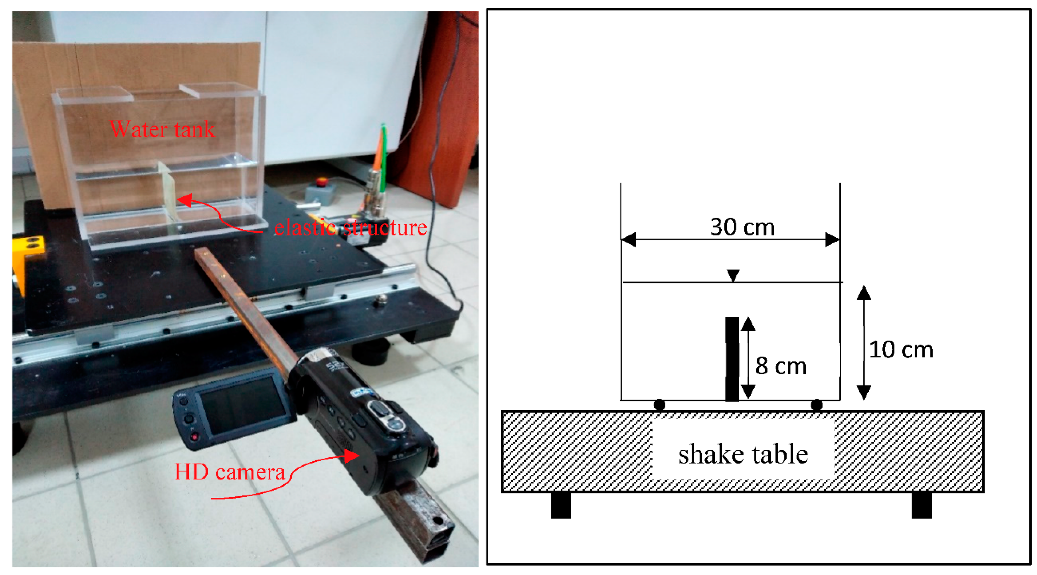
An experimental setup was developed to investigate the behavior of a highly elastic plate in a water tank under earthquake excitation. The experimental setup can be seen in Figure 2. A water tank was fixed on a shake table, which was connected to a computer. A motion was transmitted to the shake table with software compatible with the shake table. The acceleration of the shake table was also recorded with a single axis DC response accelerometer, which was also connected directly to the computer. There was no amplifier between the computer and the accelerometer.
The fluid was water, having a density of 1000 kg/m3, dynamic viscosity of 0.001 Pa, and bulk modulus of 2.2 GPa. The free-surfaces of water and the deformation and displacement of the elastic plate under a ground movement were recorded. Average modulus of elasticity of the elastic plate was 10.0 MPa. The height and the width of the elastic plate were 8 cm and 0.3 cm, respectively. All the experiments were repeated five times. Free-surface profiles and the deformations of elastic plate obtained from repeated experiments were consistent.
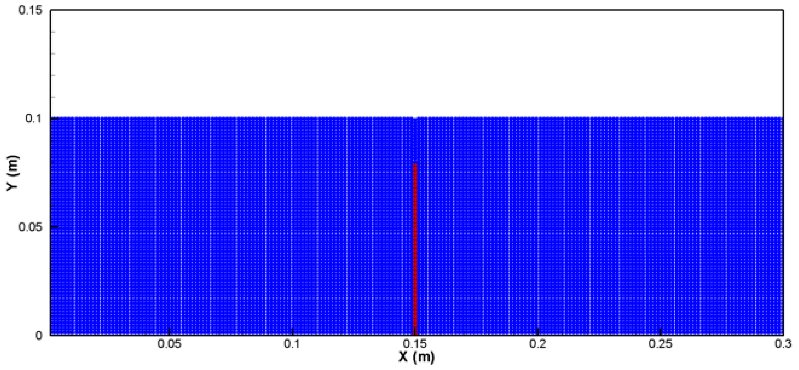
In the numerical simulations, the number of SPH particles and finite elements for elastic plate were 13,146 and 120, respectively. The initial distance between SPH particles was 1.5 mm. Time step was controlled by the CFL stability condition. The depth of water in the tank is 10 cm. The parameters used in the numerical model are summarized in Table 1. The initial distribution of SPH particles and the initial mesh of the elastic structure are shown in Figure 3.
3.1. Near-Fault Type Excitation
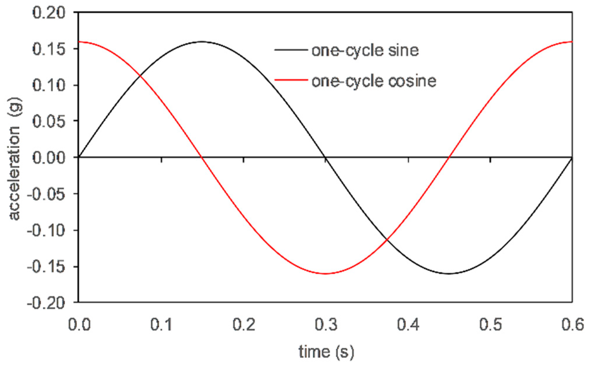
Seismic response of a structure due to near-fault excitation can be significantly different from the seismic response due to the far-field excitation [52]. Structures are exposed to high input energy in the beginning of the earthquake due to the ground motions in the near-fault region. Therefore, near-fault type excitations can considerably damage the structures [53]. In order to represent near-fault type excitation, two idealized pulses, one-cycle sine, and one-cycle cosine, shown in Figure 4, were utilized. Periods and maximum accelerations were the same for sine and cosine impulses.
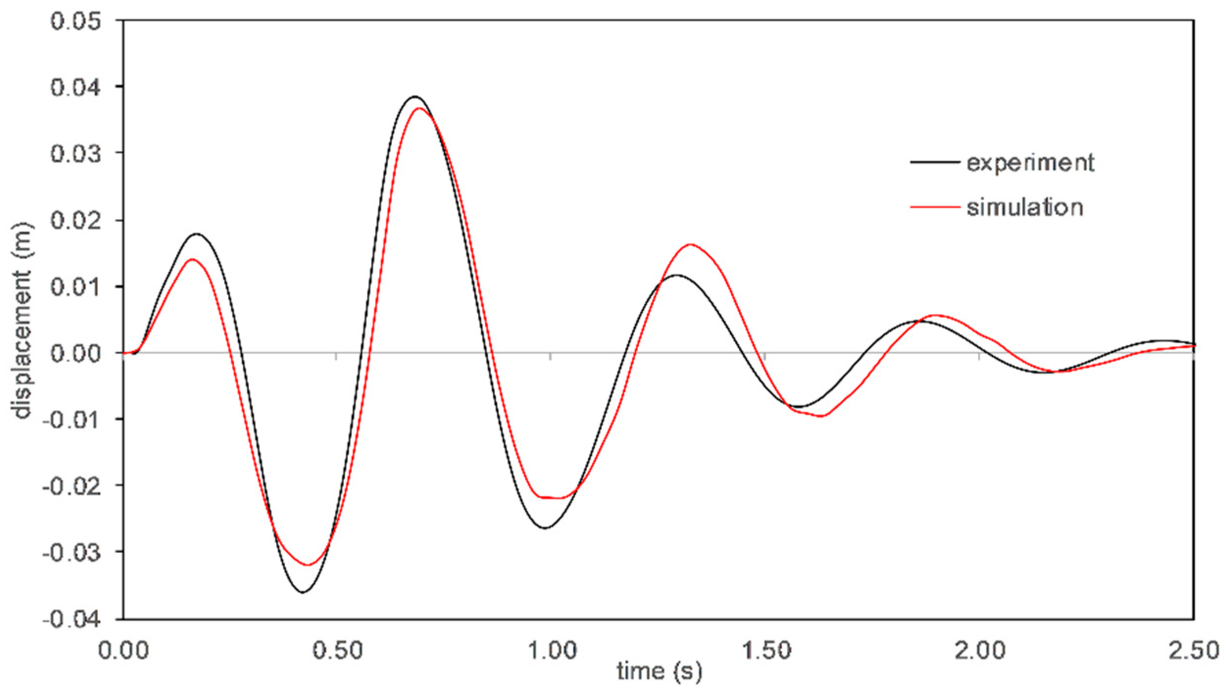
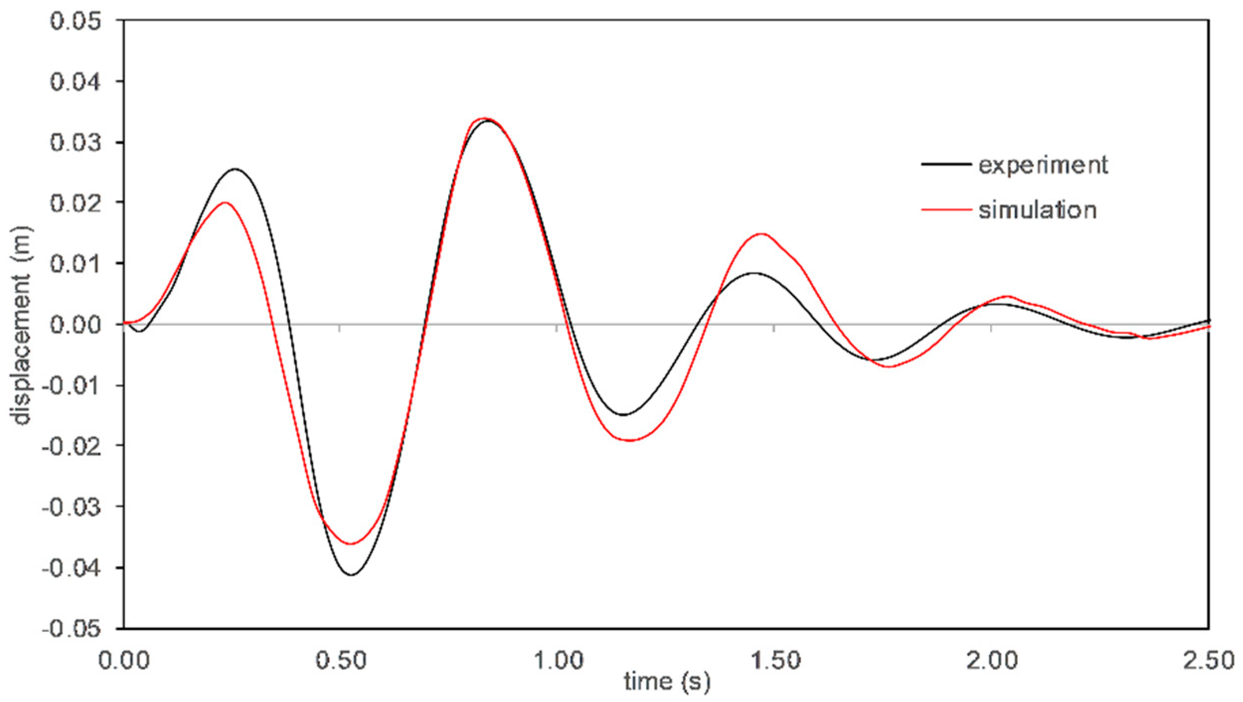
In Figure 5 and Figure 6, horizontal tip displacements of the elastic plate due to one-cycle cosine and one-cycle sine impulses are shown, respectively. As can be seen, simulated displacements were close to the experimental data. Similar displacement profiles were obtained for sine and cosine impulses. Maximum tip displacement due to one-cycle cosine was about 4 cm, whereas it was about 3.5 cm when one-cycle sine impulse was utilized. The second and the third tip displacement peaks were also higher for cosine impulse.
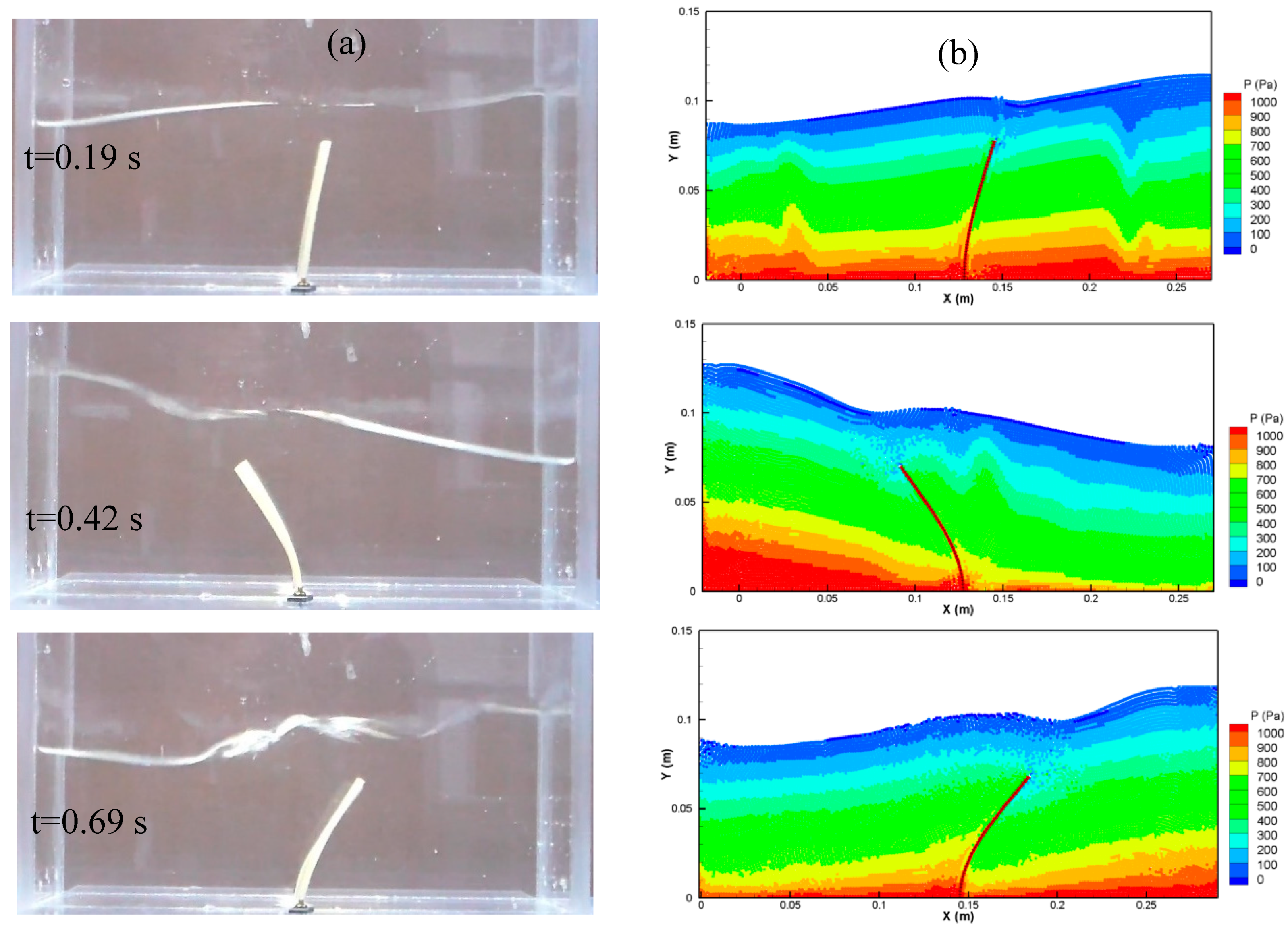
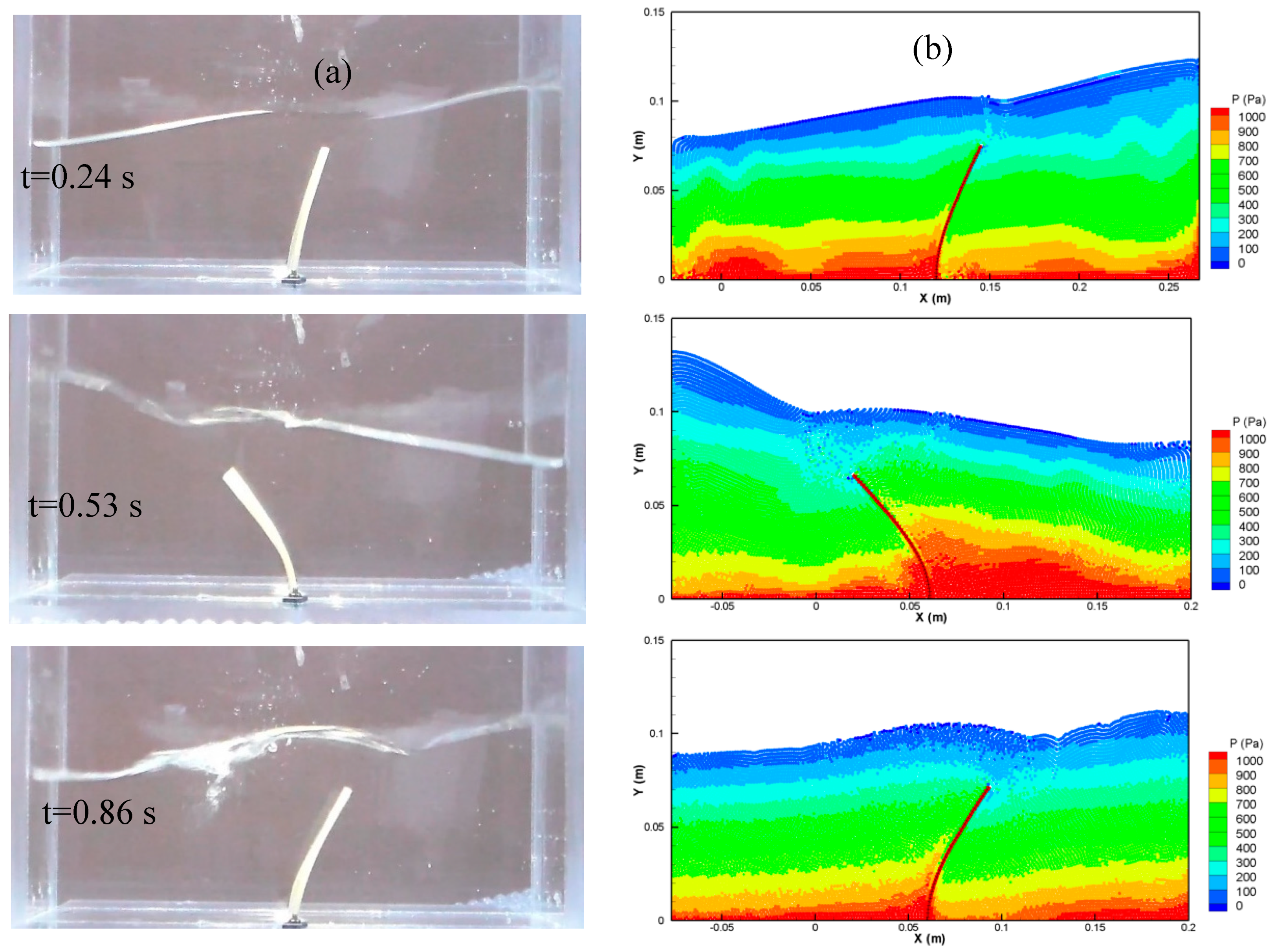
In Figure 7 and Figure 8, free-surface profiles when cosine and sine impulses were utilized are given. The instants when the profiles are given were chosen according to the instants when peak displacements are observed. It is seen that simulated free-surfaces are similar to the experimental data. In addition, the behavior of the elastic plate is captured correctly.
3.2. Earthquake Excitation
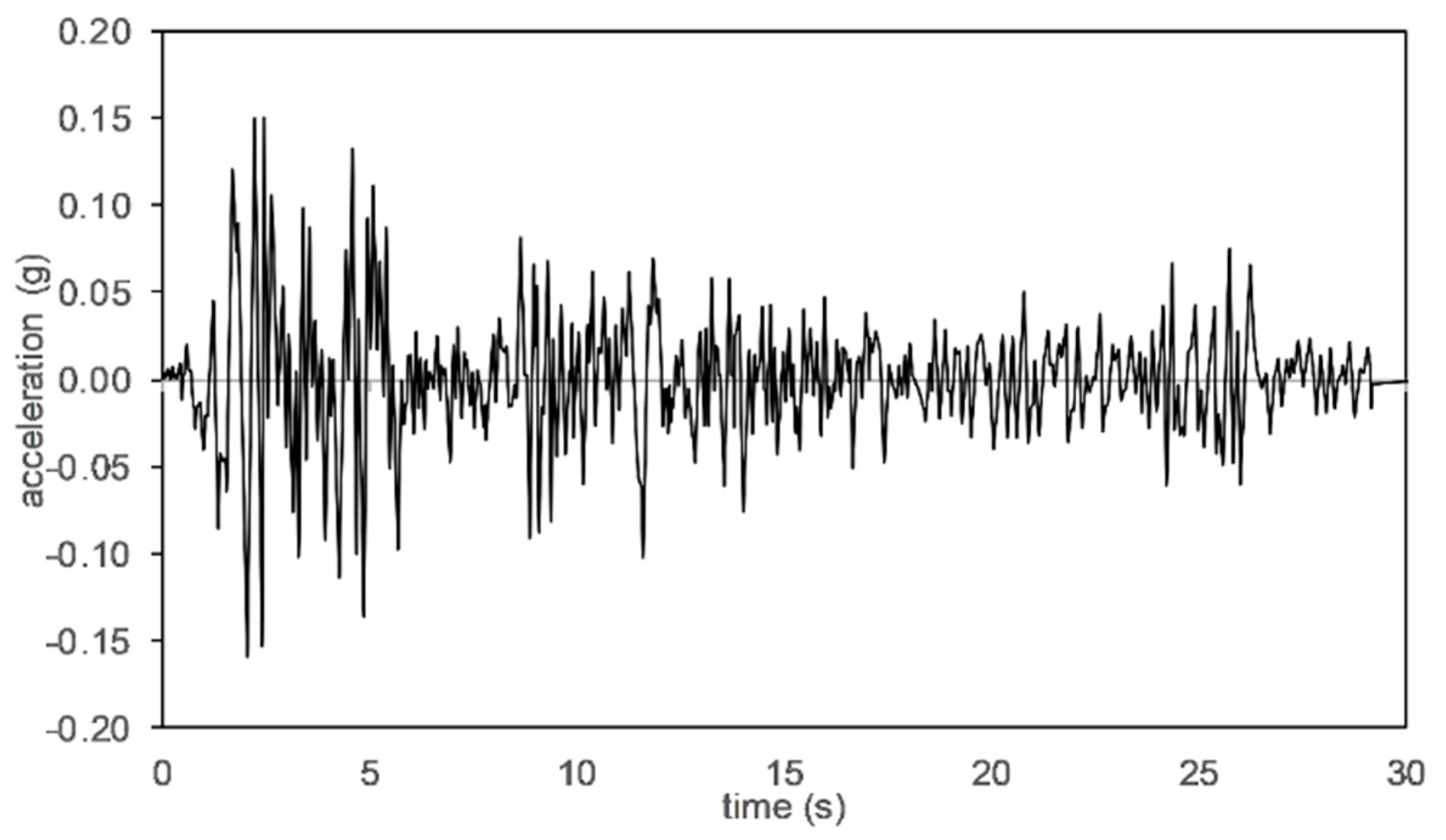
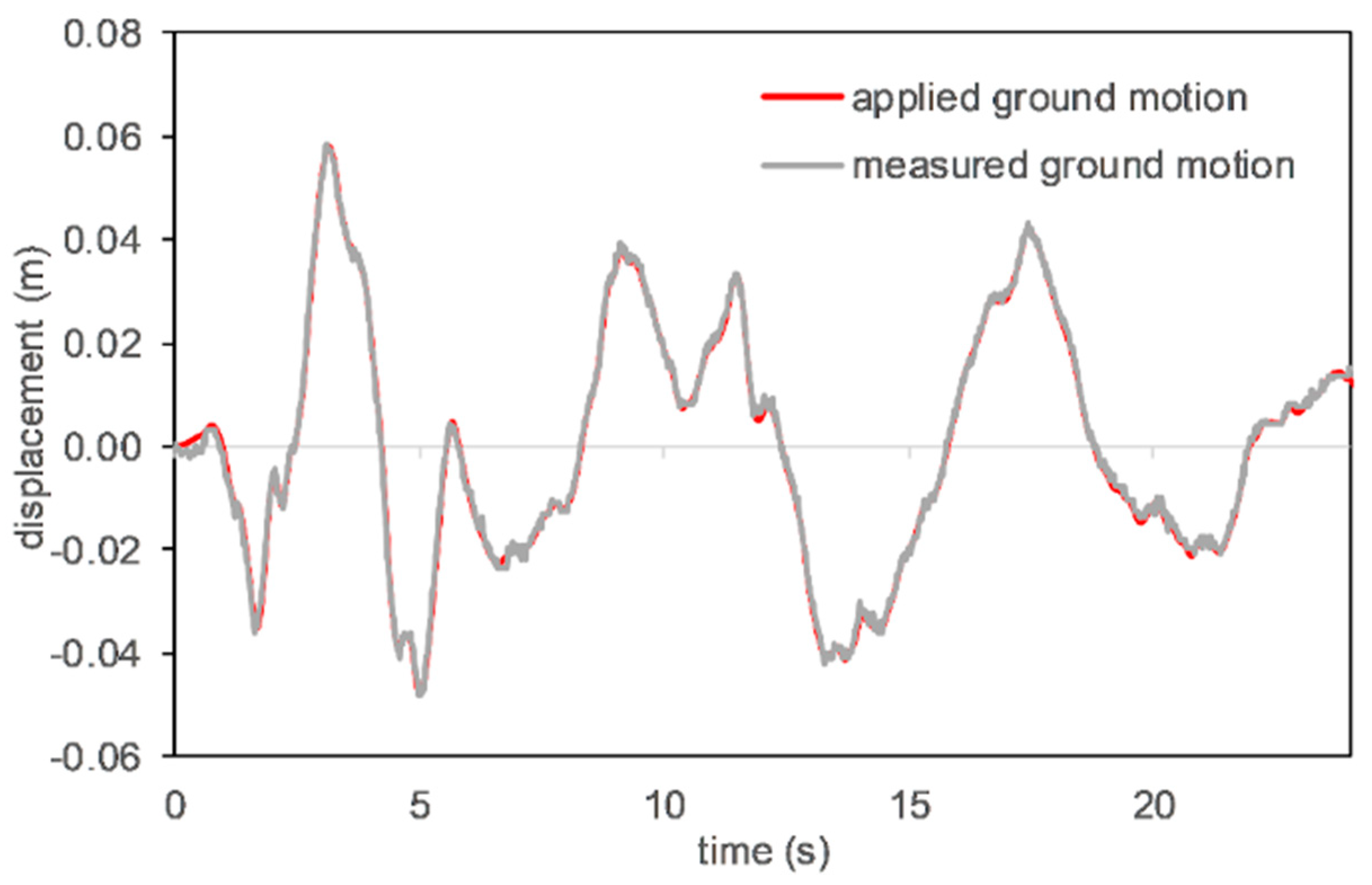
For the time history analysis, the 1940 El Centro earthquake (or 1940 Imperial Valley earthquake) was chosen. The acceleration spectrum is given in Figure 9. Applied ground motion with shake table is also compared with the measured one in Figure 10. It can be said that applied ground motion is the same with the measured one and the system works correctly.
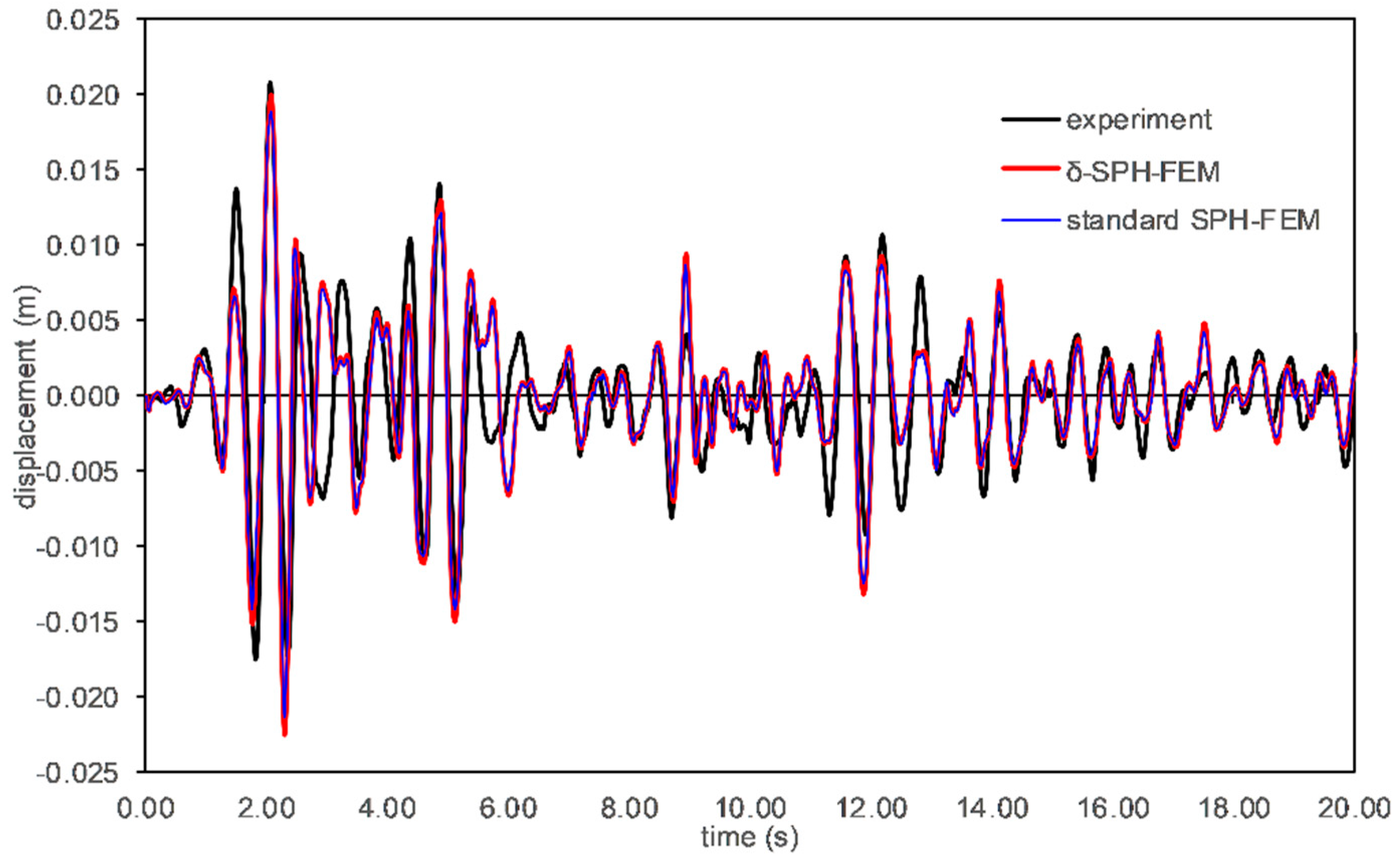
Horizontal tip displacement of the elastic plate is given in Figure 11. The maximum displacement was approximately 2 cm, which is 25% of the total length of the plate. Although minor deviations were observed between the present numerical results and the experimental data, overall, the agreement was seen to be very good. In addition, horizontal tip displacements were compared when δ-SPH scheme and standard SPH algorithm were applied. As can be seen, they are very similar. In contact mechanics algorithm, some SPH particles located in the SSOSD or intermediate region are suspended. The forces on the structure are calculated through the displacement of SPH particles interacting with the structure. Since there are always suspended particles in the SSOSD region, smoother contact forces were obtained. Therefore, similar tip displacements were obtained when δ-SPH scheme and standard SPH algorithm were utilized.
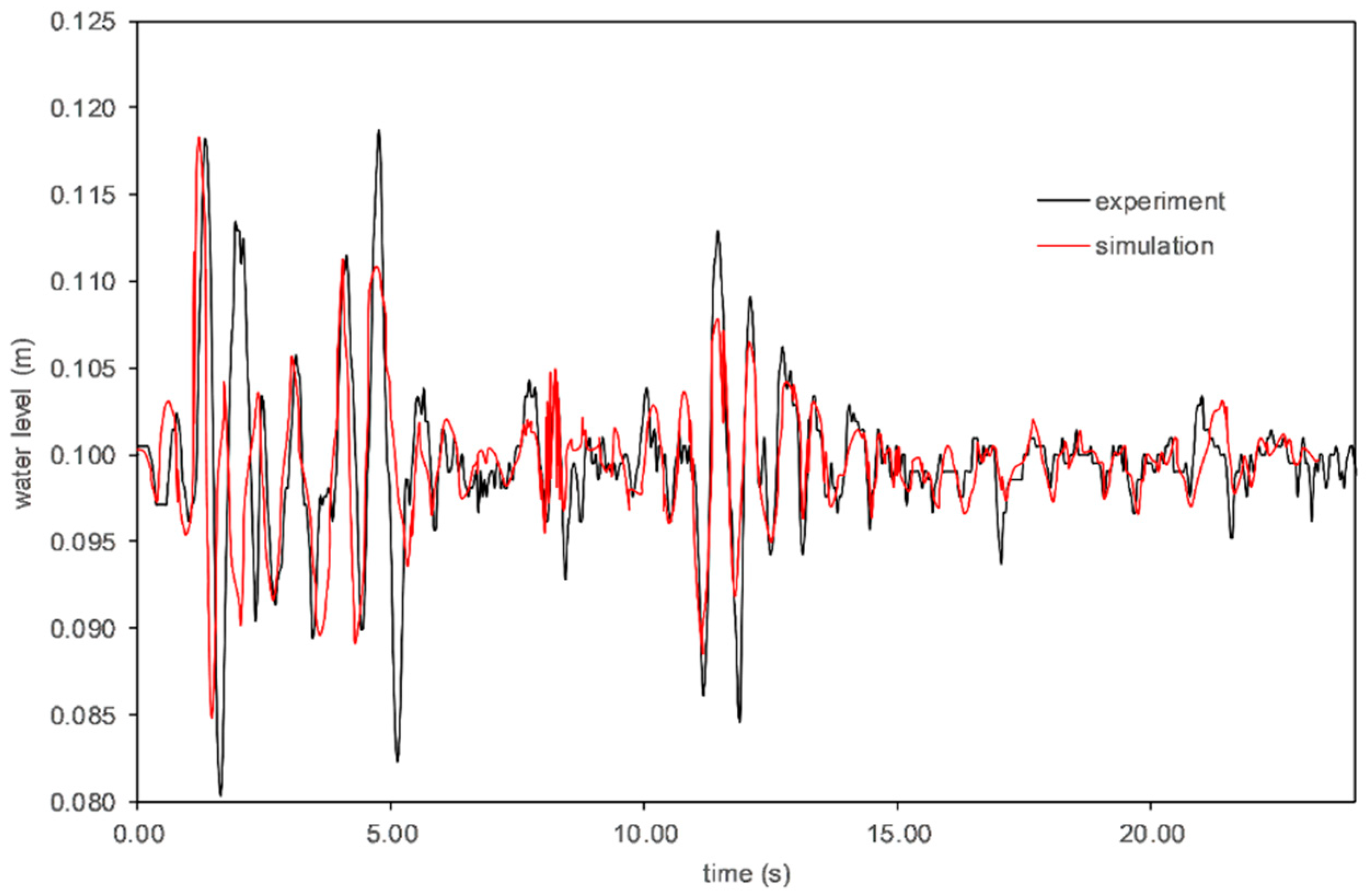
Time history of the water level near the right wall is given in Figure 12. Sloshing length near the wall of liquid tank was found to change approximately 20%. According to the figure, it can be said that numerical model can capture the free-surfaces near the wall correctly.
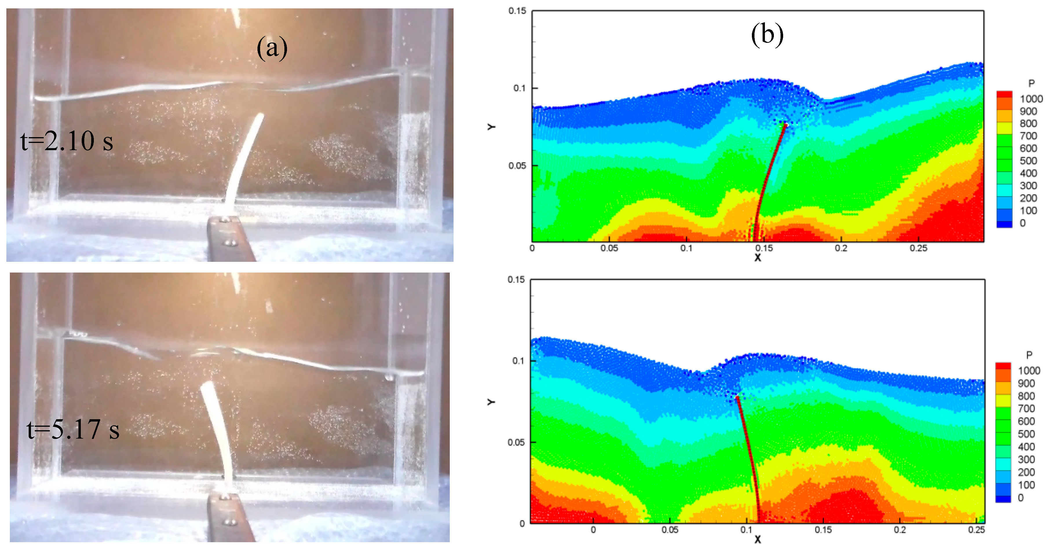
Free-surface profiles at arbitrarily chosen times are given in Figure 13. Pressures (in Pascal) of SPH particles were colorized in the numerical results. At t = 2.10 s, maximum pressure was found to be 1000 Pa and it was observed near the right wall, whereas at t = 5.17 s, maximum pressure was calculated as 1200 Pa and it was observed both near the right wall and at the right side of the elastic plate. Free-surface profiles were simulated correctly though the complex ground motion. The simulated and measured profiles of the elastic rubber were also in good agreement.
Figure 14 shows the pressure contours at t = 1.44 s. At the left side of the figure, δ-SPH scheme is given, whereas at the right side, standard SPH equations are shown. As can be seen in the figure, pressures on the SPH particles were smoother in the δ-SPH scheme. In addition, pressure distribution was also represented better in the δ-SPH scheme. Although the differences observed in pressure distribution, the deformations of elastic plate were similar. This is due to the fact that in the proposed method, the forces on the structure were calculated with contact mechanics. In the literature, most of the researchers calculated the forces on the structure from the pressures of the surrounding SPH particles, which would cause differences in the deformation profile of the structure, as explained above.
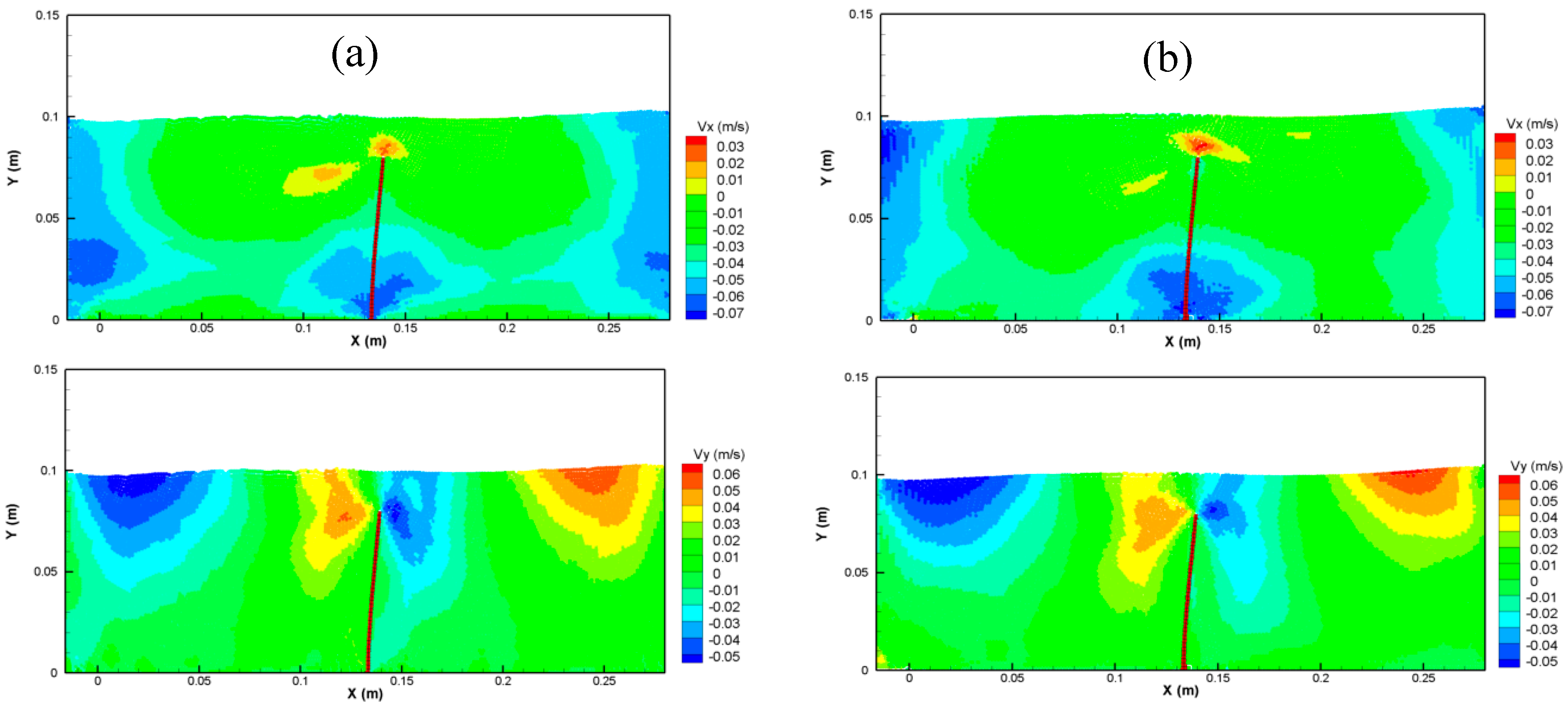
Horizontal and vertical velocity profiles are shown in Figure 15. The results of δ-SPH scheme and standard SPH are shown in the left and right columns, respectively. The regions where maximum and minimum velocities were observed are similar. However, there were small differences in the velocity profiles. The magnitude of maximum velocity found with the standard SPH scheme was slightly higher.
4. Conclusions
In this study, sloshing behavior of a fluid due to near-fault and earthquake excitations in a rectangular tank that has a highly elastic plate in the middle was investigated by including fluid-structure interaction effects. For this purpose, new experiments were conducted. In the experiments, free-surface profiles of fluid and deformation of the elastic plate were recorded. In addition, simulations were utilized by coupling δ-SPH and FEM with contact mechanics. Results obtained from the proposed method showed good agreement with the experimental data under highly nonlinear seismic excitations. When contact mechanics were used as a coupling algorithm, pressure noise does not disrupt the behavior of elastic plate significantly, because forces on the structure are not calculated through the pressures of surrounding SPH particles. Moreover, it was found that although the magnitude of maximum input accelerations of near-fault type and earthquake excitations were similar, maximum tip displacement of elastic plate due to near-fault type excitation was twice the one obtained due to earthquake excitation.
Funding
This research received no external funding.
Conflicts of Interest
The authors declare no conflict of interest.
References
- Stofan, A.J.; Sumner, I.E. Technical Note; Natl. Aeronaut. Sp. Adm. Ohio, Lowis Res. Center: Cleveland, OH, USA, 1963. [Google Scholar]
- Chiba, M. Nonlinear hydroelastic vibration of a cylindrical tank with an elastic bottom, containing liquid. Part I: Experiment. J. Fluids Struct. 1992, 6, 181–206. [Google Scholar] [CrossRef]
- Yalla, S.K.; Kareem, A.; Kantor, J.C. Semi-active tuned liquid column dampers for vibration control of structures. Eng. Struct. 2001, 23, 1469–1479. [Google Scholar] [CrossRef]
- Bredmose, H.; Brocchini, M.; Peregrine, D.H.; Thais, L. Experimental investigation and numerical modelling of steep forced water waves. J. Fluid Mech. 2003, 490, 217–249. [Google Scholar] [CrossRef]
- Akyildiz, H.; Ünal, E. Experimental investigation of pressure distribution on a rectangular tank due to the liquid sloshing. Ocean Eng. 2005, 32, 1503–1516. [Google Scholar] [CrossRef]
- Idelsohn, S.R.; Marti, J.; Souto-iglesias, A.; Oñate, E. Interaction between an elastic structure and free-surface flows: Experimental versus numerical comparisons using the PFEM. Comput. Mech. 2008, 43, 125–132. [Google Scholar] [CrossRef]
- Kim, Y. Numerical simulation of sloshing flows with impact load. Appl. Ocean Res. 2001, 23, 53–62. [Google Scholar] [CrossRef]
- Celebi, M.S.; Akyildiz, H. Nonlinear modeling of liquid sloshing in a moving rectangular tank. Ocean Eng. 2002, 29, 1527–1553. [Google Scholar] [CrossRef]
- Pal, P. Sloshing of Liquid in Partially Filled Container—An Experimental Study. Int. J. Recent Trends Eng. 2009, 1, 1–5. [Google Scholar]
- Chen, Y.; Xue, M.A. Numerical simulation of liquid sloshing with different filling levels using OpenFOAM and experimental validation. Water 2018, 10, 1752. [Google Scholar] [CrossRef] [Green Version]
- Serván-Camas, B.; Cercós-Pita, J.L.; Colom-Cobb, J.; García-Espinosa, J.; Souto-Iglesias, A. Time domain simulation of coupled sloshing–seakeeping problems by SPH–FEM coupling. Ocean Eng. 2016, 123, 383–396. [Google Scholar] [CrossRef] [Green Version]
- Hwang, S.C.; Park, J.C.; Gotoh, H.; Khayyer, A.; Kang, K.J. Numerical simulations of sloshing flows with elastic baffles by using a particle-based fluid-structure interaction analysis method. Ocean Eng. 2016, 118, 227–241. [Google Scholar] [CrossRef]
- Michael Isaacson, B.; Ryu, C.-S. Earthquake-Induced Sloshing in Vertical Container of Arbitrary Section. J. Eng. Mech. 1998, 124, 158–166. [Google Scholar] [CrossRef]
- Hernández-Barrios, H.; Heredia-Zavoni, E.; Aldama-Rodríguez, Á.A. Nonlinear sloshing response of cylindrical tanks subjected to earthquake ground motion. Eng. Struct. 2007, 29, 3364–3376. [Google Scholar] [CrossRef]
- Panigrahy, P.K.; Saha, U.K.; Maity, D. Experimental studies on sloshing behavior due to horizontal movement of liquids in baffled tanks. Ocean Eng. 2009, 36, 213–222. [Google Scholar] [CrossRef]
- Luo, H.; Zhang, R.; Weng, D. Mitigation of liquid sloshing in storage tanks by using a hybrid control method. Soil Dyn. Earthq. Eng. 2016, 90, 183–195. [Google Scholar] [CrossRef]
- Hashimoto, H.; Hata, Y.; Kawamura, K. Estimation of oil overflow due to sloshing from oil storage tanks subjected to a possible Nankai Trough earthquake in Osaka bay area. J. Loss Prev. Process Ind. 2017, 50, 337–346. [Google Scholar] [CrossRef]
- Cheng, X.; Cao, L.; Zhu, H. Liquid-solid Interaction Seismic Response of an Isolated Overground Rectangular Reinforced-concrete Liquid-storage Structure. J. Asian Archit. Build. Eng. 2015, 14, 175–180. [Google Scholar] [CrossRef] [Green Version]
- Yu, C.-C.; Whittaker, A.; Coleman, J. Verification of a fluid-structure-interaction model for seismic analysis of Gen IV nuclear power plants. In Proceedings of the 11th National Conference in Earthquake Engineering, Earthquake Engineering Research Institute, Los Angeles, CA, USA, 25–29 June 2018. [Google Scholar]
- Waezi, Z.; Attari, N.K.A.; Rofooei, F.R. Controlling the seismic response of structures under near-field earthquakes with fluid/structure interaction of cylindrical liquid tanks. Eur. J. Environ. Civ. Eng. 2019, 23, 1–24. [Google Scholar] [CrossRef]
- Demir, A.; Dinçer, A.E. MPS ve FEM Tabanlı Akışkan-Yapı Etkileşimi Modelinin Çoruh Nehri Üzerindeki Ardıl Baraj-Yıkılma Problemine Uygulanması. Doğal Afetler ve Çevre Derg 2017, 90, 1–6. [Google Scholar] [CrossRef]
- Calderer, A.; Kang, S.; Sotiropoulos, F. Level set immersed boundary method for coupled simulation of air/water interaction with complex floating structures. J. Comput. Phys. 2014, 277, 201–227. [Google Scholar] [CrossRef] [Green Version]
- Pathak, A.; Raessi, M. A 3D, fully Eulerian, VOF-based solver to study the interaction between two fluids and moving rigid bodies using the fictitious domain method. J. Comput. Phys. 2016, 311, 87–113. [Google Scholar] [CrossRef] [Green Version]
- Wang, L.; Currao, G.M.D.; Han, F.; Neely, A.J.; Young, J.; Tian, F.B. An immersed boundary method for fluid–structure interaction with compressible multiphase flows. J. Comput. Phys. 2017, 346, 131–151. [Google Scholar] [CrossRef] [Green Version]
- Nangia, N.; Patankar, N.A.; Bhalla, A.P.S. A DLM immersed boundary method based wave-structure interaction solver for high density ratio multiphase flows. arXiv 2019, arXiv:1901.07892. [Google Scholar] [CrossRef] [Green Version]
- Demir, A.; Dinçer, A.E.; Bozkus, Z.; Tijsseling, A.S. Numerical and experimental investigation of damping in a dam-break problem with fluid-structure interaction. J. Zhejiang Univ. Sci. A 2019, 20, 258–271. [Google Scholar] [CrossRef]
- Dinçer, A.E.; Demir, A.; Bozkus, Z.; Tijsseling, A.S. Fully Coupled Smoothed Particle Hydrodynamics-Finite Element Method Approach for Fluid-Structure Interaction Problems With Large Deflections. J. Fluids Eng. Trans. ASME 2019, 141, 1–13. [Google Scholar] [CrossRef]
- Gingold, R.A.; Monaghan, J.J. Smoothed particle hydrodynamics: Theory and application to non-spherical stars. Mon. Not. R. Astron. Soc. 1977, 181, 375–389. [Google Scholar] [CrossRef]
- Lucy, L.B. A numerical approach to the testing of the fission hypothesis. Astron. J. 1977, 82, 1013–1024. [Google Scholar] [CrossRef]
- Dinçer, A.E. Numerical Investigation of Free Surface and Pipe Flow Problems by Smoothed Particle Hydrodynamics. Ph. D. Thesis, Middle East Technical University, Ankara, Turkey, 2017. [Google Scholar]
- Dinçer, A.E.; Bozkuş, Z.; Tijsseling, A.S. Prediction of Pressure Variation at an Elbow Subsequent to a Liquid Slug Impact by Using Smoothed Particle Hydrodynamics. J. Press. Vessel Technol. Trans. ASME 2018, 140, 031303. [Google Scholar] [CrossRef]
- Dinçer, A.E.; Bozkuş, Z.; Şahin, A.N. Effect of downstream channel slope on numerical modelling of dam break induced flows. In Proceedings of the Sustainable Hydraulics in the Era of Global Change—Proceedings of the 4th European Congress of the International Association of Hydroenvironment engineering and Research, IAHR, Granada, Spain, 4–9 July 2016. [Google Scholar]
- Attaway, S.W.; Heinstein, M.W.; Swegle, J.W. Coupling of smooth particle hydrodynamics with the finite element method. Nucl. Eng. Des. 1994, 150, 199–205. [Google Scholar] [CrossRef]
- Johnson, G.R. Linking of Lagrangian particle methods to standard finite element methods for high velocity impact computations. Nucl. Eng. Des. 1994, 150, 265–274. [Google Scholar] [CrossRef]
- Johnson, G.R.; Beissel, S.R. Normalized smoothing functions for sph impact computations. Int. J. Numer. Methods Eng. 1996, 39, 2725–2741. [Google Scholar] [CrossRef]
- De Vuyst, T.; Vignjevic, R.; Campbell, J.C. Coupling between meshless and finite element methods. Int. J. Impact Eng. 2005, 31, 1054–1064. [Google Scholar] [CrossRef]
- Fernández-Méndez, S.; Bonet, J.; Huerta, A. Continuous blending of SPH with finite elements. Comput. Struct. 2005, 83, 1448–1458. [Google Scholar] [CrossRef] [Green Version]
- Zhang, Z.; Qiang, H.; Gao, W. Coupling of smoothed particle hydrodynamics and finite element method for impact dynamics simulation. Eng. Struct. 2010, 33, 255–264. [Google Scholar] [CrossRef]
- Hu, D.; Long, T.; Xiao, Y.; Han, X.; Gu, Y. Fluid-structure interaction analysis by coupled FE-SPH model based on a novel searching algorithm. Comput. Methods Appl. Mech. Eng. 2014, 276, 266–286. [Google Scholar] [CrossRef] [Green Version]
- Fourey, G.; Hermange, C.; Le Touzé, D.; Oger, G. An efficient FSI coupling strategy between Smoothed Particle Hydrodynamics and Finite Element methods. Comput. Phys. Commun. 2017, 217, 66–81. [Google Scholar] [CrossRef]
- Long, T.; Hu, D.; Wan, D.; Zhuang, C.; Yang, G. An arbitrary boundary with ghost particles incorporated in coupled FEM–SPH model for FSI problems. J. Comput. Phys. 2017, 350, 166–183. [Google Scholar] [CrossRef]
- Liu, G.; Liu, M.B. Smoothed Particle Hydrodynamics: A Mesh-Free Particle Method; World Scientific Publishing Co. Pte. Ltd.: Singapore, 2003; ISBN 981-238-456-1. [Google Scholar]
- Marrone, S.; Antuono, M.; Colagrossi, A.; Colicchio, G.; Le Touzé, D.; Graziani, G. δ-SPH model for simulating violent impact flows. Comput. Methods Appl. Mech. Eng. 2011, 200, 1526–1542. [Google Scholar] [CrossRef]
- Monaghan, J.J. Smoothed Particle Hydrodynamics. Annu. Rev. Astron. Astrophys. 1992, 30, 543–574. [Google Scholar] [CrossRef]
- Shao, J.R.; Li, H.Q.; Liu, G.R.; Liu, M.B. An improved SPH method for modeling liquid sloshing dynamics. Comput. Struct. 2012, 100, 18–26. [Google Scholar] [CrossRef] [Green Version]
- Randles, P.W.; Libersky, L.D. Smoothed Particle Hydrodynamics: Some recent improvements and applications. Comput. Methods Appl. Mech. Engrg. 1996, 7825, 375–408. [Google Scholar] [CrossRef]
- Morris, J.P.; Fox, P.J.; Zhu, Y. Modeling Low Reynolds Number Incompressible Flows Using SPH. J. Comput. Phys. 1997, 136, 214–226. [Google Scholar] [CrossRef]
- Anderson, J.D. Computational Fluid Dynamics: The Basics with Applications; McGraw-Hill: New York, NY, USA, 1995. [Google Scholar]
- Monaghan, J.J.; Kos, A. Solitary Waves on a Cretan Beach. J. Waterw. Port Coast. Ocean Eng. 1999, 125, 145–155. [Google Scholar] [CrossRef]
- Bathe, K.-J. Finite Element Procedures; Prentice Hall, Pearson Education, Inc: Watertown, NY, USA, 2006; ISBN 9780979004957. [Google Scholar]
- Wilson, E.L. Three-Dimensional Static and Dynamic Analysis of Structures; Computers and Structures: Berkeley, CA, USA, 2002; Volume 90, ISBN 0923907009. [Google Scholar]
- Zhang, S.; Wang, G. Effects of near-fault and far-fault ground motions on nonlinear dynamic response and seismic damage of concrete gravity dams. Soil Dyn. Earthq. Eng. 2013, 53, 217–229. [Google Scholar] [CrossRef]
- Liao, W.I.; Loh, C.H.; Lee, B.H. Comparison of dynamic response of isolated and non-isolated continuous girder bridges subjected to near-fault ground motions. Eng. Struct. 2004, 26, 2173–2183. [Google Scholar] [CrossRef]
Figure 1.
Illustration of fluid and structural domains in surface of the structural domain (SSOSD).

Figure 2.
Experimental Setup.

Figure 3.
Initial particle and mesh distribution.

Figure 4.
Idealized pulses to represent near-fault ground motion.

Figure 5.
Horizontal tip displacement of the elastic plate due to one-cycle cosine impulse.

Figure 6.
Horizontal tip displacement of the elastic plate due to one-cycle sine impulse.

Figure 7.
Free surface profiles under one-cycle cosine acceleration impulse for (a) experiment and (b) simulation.
Figure 7.
Free surface profiles under one-cycle cosine acceleration impulse for (a) experiment and (b) simulation.

Figure 8.
Free surface profiles under one-cycle sine acceleration impulse for (a) experiment and (b) simulation.
Figure 8.
Free surface profiles under one-cycle sine acceleration impulse for (a) experiment and (b) simulation.

Figure 9.
Acceleration spectrum of the 1940 El Centro earthquake (or 1940 Imperial Valley earthquake).
Figure 9.
Acceleration spectrum of the 1940 El Centro earthquake (or 1940 Imperial Valley earthquake).

Figure 10.
Applied and measured ground motion.

Figure 11.
Horizontal tip displacement of the elastic plate.

Figure 12.
Free-surface wave height near the right wall.

Figure 13.
Free-surface profiles of (a) experimental data and (b) numerical results.

Figure 14.
Comparison between free-surface profiles of (a) the δ-SPH scheme and (b) the standard SPH at t = 1.44 s.
Figure 14.
Comparison between free-surface profiles of (a) the δ-SPH scheme and (b) the standard SPH at t = 1.44 s.

Figure 15.
Comparison between velocity contours of (a) the δ-SPH scheme and (b) the standard SPH at t = 1.44 s.
Figure 15.
Comparison between velocity contours of (a) the δ-SPH scheme and (b) the standard SPH at t = 1.44 s.


Table 1.
The parameters used in the numerical model.
| The height of the plate (cm) | 8.0 |
| The width of the plate (cm) | 0.3 |
| Modulus of elasticity of the plate (MPa) | 10.0 |
| The initial distance between SPH particles (cm) | 0.15 |
| Max. time step (s) | 0.000016 |
| The number of SPH particles | 13,146 |
| The number of finite elements | 120 |
© 2019 by the author. Licensee MDPI, Basel, Switzerland. This article is an open access article distributed under the terms and conditions of the Creative Commons Attribution (CC BY) license (http://creativecommons.org/licenses/by/4.0/).
Share and Cite
MDPI and ACS Style
Dinçer, A.E. Investigation of the Sloshing Behavior Due to Seismic Excitations Considering Two-Way Coupling of the Fluid and the Structure. Water 2019, 11, 2664. https://doi.org/10.3390/w11122664
AMA Style
Dinçer AE. Investigation of the Sloshing Behavior Due to Seismic Excitations Considering Two-Way Coupling of the Fluid and the Structure. Water. 2019; 11(12):2664. https://doi.org/10.3390/w11122664
Chicago/Turabian StyleDinçer, A. Ersin. 2019. "Investigation of the Sloshing Behavior Due to Seismic Excitations Considering Two-Way Coupling of the Fluid and the Structure" Water 11, no. 12: 2664. https://doi.org/10.3390/w11122664
Note that from the first issue of 2016, this journal uses article numbers instead of page numbers. See further details here.