


Abstract
We present the first measurements of H i galaxy scaling relations from a blind survey at z > 0.15. We perform spectral stacking of 9023 spectra of star-forming galaxies undetected in H i at 0.23 < z < 0.49, extracted from MIGHTEE-H i Early Science data cubes, acquired with the MeerKAT radio telescope. We stack galaxies in bins of galaxy properties (stellar mass M*, star formation rateSFR, and specific star formation rate sSFR, with sSFR ≡ M*/SFR), obtaining ≳5σ detections in most cases, the strongest H i-stacking detections to date in this redshift range. With these detections, we are able to measure scaling relations in the probed redshift interval, finding evidence for a moderate evolution from the median redshift of our sample zmed ∼ 0.37 to z ∼ 0. In particular, low-M* galaxies ( ) experience a strong H i depletion (∼0.5 dex in
  ), while massive galaxies (
 ) keep their H i mass nearly unchanged. When looking at the star formation activity, highly star-forming galaxies evolve significantly in MH I (fH I, where fH I ≡ MH I/M*) at fixed SFR (sSFR), while at the lowest probed SFR (sSFR) the scaling relations show no evolution. These findings suggest a scenario in which low-M* galaxies have experienced a strong H i depletion during the last ∼5 Gyr, while massive galaxies have undergone a significant H i replenishment through some accretion mechanism, possibly minor mergers. Interestingly, our results are in good agreement with the predictions of the simba simulation. We conclude that this work sets novel important observational constraints on galaxy scaling relations.
Export citation and abstract BibTeX RIS

Original content from this work may be used under the terms of the Creative Commons Attribution 4.0 licence. Any further distribution of this work must maintain attribution to the author(s) and the title of the work, journal citation and DOI.
1. Introduction
In the modern paradigm of galaxy formation and evolution, the baryon cycle of galaxies can be investigated through the parameterization of scaling relations linking their physical properties at different cosmic times.
In this context, the neutral atomic hydrogen (H i) constitutes the fundamental component for H2 assembly and therefore represents the raw fuel for star formation. Unveiling H i scaling relations in galaxies is thus a task of paramount importance to understand how the availability of fresh cold gas regulates star formation and galaxy evolution.
Tight relations at z ∼ 0 between the H i content of star-forming galaxies and their stellar mass (M*, Huang et al. 2012; Maddox et al. 2015), star formation rate (SFR, Feldmann 2020), and disk size (e.g., Wang et al. 2016, and references therein), among others, have been revealed by large-scale H i galaxy surveys, such as the H i Parkes All-Sky Survey (HIPASS; Barnes et al. 2001), the Arecibo Legacy Fast ALFA Survey (ALFALFA; Giovanelli et al. 2005), and the GALEX Arecibo SDSS Survey (GASS; Catinella et al. 2010).
Nonetheless, the H i content of galaxies has been so far included in the global scaling relation picture only at very low redshift (z < 0.15), due to the intrinsic faintness of the 21 cm hyperfine transition emission line and, hitherto, the limited sensitivity of radio telescopes.
A few blind deep observational efforts—e.g., the Blind Ultra-Deep HI Environmental Survey (BUDHIES; Verheijen et al. 2007), the COSMOS HI Large Extragalactic Survey (CHILES; Hess et al. 2019), and the Arecibo Ultra-Deep Survey (AUDS; Hoppmann et al. 2015)—have reported sparse detections at z > 0.15. However, their samples are not large enough to constrain scaling relations.
In the build-up toward the the Square Kilometre Array (SKA), spectral line stacking (e.g., Zwaan 2000) can be adopted as an alternative cheaper observational technique to direct detection, performing an average H i mass (MH I) detection of a given galaxy sample. Stacking has been proven to be a powerful tool to investigate many different aspects of galaxy evolution, among which are the presence and abundance of H i in galaxy clusters (e.g., Lah et al. 2009; Healy et al. 2021), scaling relations (e.g., Brown et al. 2017), the MH I content of active galactic nucleus (AGN) host galaxies (Geréb et al. 2015), and the redshift evolution of the H i cosmic density parameter ΩH I (e.g., Delhaize et al. 2013; Rhee et al. 2013; Chowdhury et al. 2020, and references therein). In particular, Rhee et al. (2013, 2016, 2018) reported tentative detections (≲3σ) at z ∼ 0.2, z ∼ 0.37, and z ∼ 0.32, respectively. Bera et al. (2019) presented a strong ∼7.3σ detection at z ∼ 0.34. Chowdhury et al. (2020, 2021, 2022a, 2022b) reported clear ∼4.5σ, ∼5σ, ∼5.6σ and ∼5.2σ, and 7.1σ detections with stacking at z ∼ 1, z ∼ 1.3, z ∼ 1 and z ∼ 1.3, and z ∼ 1, respectively.
In this Letter, we perform spectral stacking on MIGHTEE-H i (see Section 2 for a description of the MIGHTEE survey) data cubes to study H i scaling relations out to z ∼ 0.5 and report the first direct measurement of such relations at z > 0.15. In particular, we focus here on the relations between stellar mass, H i mass, and star formation activity to study how such relations linking key galaxy parameters evolve at z < 0.5. Moreover, we compare our stacked results with simulated results from the simba cosmological simulation (Davé et al.2019).
The paper is structured as follows. In Section 2 we introduce the MIGHTEE-H i survey and our H i data. In Section 3 we present our galaxy sample. In Section 4 we summarize the basic principles of the stacking procedure we adopt throughout the paper. Section 5 presents the main results of this work and our interpretation of them. We conclude in Section 6.
We assume a spatially flat (Ωk = 0) ΛCDM Cosmology, with cosmological parameters from the latest Planck collaboration results (Planck Collaboration et al. 2020), i.e., H0 = 67.4 km s−1 Mpc−1, Ωm = 0.315, and ΩΛ = 0.685.
2. H i Data from MIGHTEE
The MeerKAT International GigaHertz Tiered Extragalactic Exploration Large Survey Program (MIGHTEE; Jarvis et al. 2016) is a survey, conducted with the MeerKAT radio interferometer (e.g., Jonas & MeerKAT Team 2016), observing four deep, extragalactic fields (COSMOS, XMMLSS, ECDFS, and ELAIS-S), characterized by a wealth of multiwavelength data made available by past and ongoing observational efforts. MeerKAT is the SKA precursor located in South Africa and comprises 64 offset Gregorian dishes (13.5 m diameter main reflector and 3.8 m subreflector), equipped with receivers in the UHF band (580 < ν < 1015 MHz), L band (900 < ν < 1670 MHz), and S band (1750 < ν < 3500 MHz).
The MeerKAT data were acquired in spectral and full Stokes mode, thereby making MIGHTEE a spectral line, continuum, and polarization survey. In this paper, we make use of the Early Science H i spectral line data from MIGHTEE, presented in Maddox et al. (2021); B. Frank et al. 2022 (in preparation). The observations were conducted between mid 2018 and mid 2019 and targeted ∼3.5 deg2 in the XMMLSS field and ∼1.5 deg2 in the COSMOS field. These observations were performed with the full array (64 dishes) in the L band, using the 4 k correlator mode (209 kHz, corresponding to 52 km s−1 at z = 0.23 and 56 km s−1 at z = 0.49). The MIGHTEE-H i Early Science visibilities were processed with the ProcessMeerKAT calibration pipeline. The pipeline is Casa based and performs standard calibration routines and strategies for the spectral line data such as flagging, bandpass, and complex gain calibration. The continuum subtraction was done in both the visibility and image domain using standard Casa routines uvsub and uvcontsub. Residual visibilities after continuum subtraction were imaged using Casa's task tclean with Briggs' weighting (robust = 0.5). Eventually, median filtering was applied to the resulting data cubes to reduce the impact of errors due to continuum subtraction. A full description of the data reduction strategy and data quality assessment will be presented in B. Frank et al. 2022 (in preparation).
Out of the full MIGHTEE-H i data set, we make use of MIGHTEE-H i data cubes covering the COSMOS field. Our analysis is limited to the redshift interval 0.23 < z < 0.49. At these redshifts, MIGHTEE-H i data are found to have well-behaved Gaussian noise, with the median H i noise rms increasing with decreasing frequency, from 85 μJy beam−1 at ν ∼ 1050 MHz to 135 μJy beam−1 at ν ∼ 950 MHz (B. Frank et al. 2022, in preparation). We exclude the spectral bands at 0.09 < z < 0.23 and z > 0.49 from our analysis, as they are characterized by strong RFI features (Maddox et al. 2021; B. Frank et al. 2022, in preparation). A first preliminary unguided visual source finding reported no direct H i detections at z > 0.23. A summary of the features of the MIGHTEE-H i data used in this work is provided in Table 1.
Table 1. Summary of the Details of MIGHTEE-H i Data Presented in Section 2 and Used in This Paper
| MIGHTEE-H i Data | |
|---|---|
| Survey Parameter | Value |
| Field | COSMOS |
| Area | 1.5 deg2 |
| Integration time | 16 hr |
| Frequency resolution | 209 kHz |
| Velocity resolution | 52 km s−1 at z = 0.23 |
| Frequency range | 0.950–1.050 GHz |
| Velocity range | 68,952–146,898 km s−1 |
| Beam (FWHM) | 14 5 × 110 5 × 110 |
Download table as: ASCIITypeset image
3. Sample Selection
We select star-forming galaxies at redshift 0.23 < z < 0.49 in the COSMOS field (Scoville et al. 2007), with spectroscopic redshift information available.
We start by considering the latest COSMOS photometric sample publicly available as part of the COSMOS2020 data release (Weaver et al. 2021). This data set includes estimates of the derived galaxy properties (we consider M* and SFR in this work) obtained through spectral energy density (SED) fitting. Then, we select star-forming galaxies, according to a color–color NUV − r/r − J plane selection. In particular, quiescent galaxies are defined as those having MNUV − Mr > 3(Mr − MJ ) + 1 and MNUV − Mr > 3.1, while the remaining galaxies are flagged as star-forming (see Laigle et al. 2016). This defines our parent sample.
Out of the parent sample, we extract only galaxies having a spectroscopic counterpart. This is done by cross-matching the parent sample with a list of spectroscopic redshifts assembled by querying publicly available catalogs from spectroscopic surveys of the COSMOS field (M. Salvato et al. 2022, in preparation.) and spectroscopic redshifts acquired by the DEVILS survey (Davies et al. 2018). Because the SED fitting was performed by adopting the photometric redshift as estimates for redshift, we checked for outliers in the photometric redshifts determination. 30 We find that the outliers constitute ≲5% of our sample and excluded them.
Moreover, we explicitly cross-checked the accuracy of the SFR determination, which can induce substantial deviations when obtained through SED fitting in the absence of FIR-band data in the case of dust-attenuated galaxies. In particular, where it applies, we compare our SFR estimates with the ones obtained relying on independent FIR measurements (not used in the SED fitting mentioned above) presented in Jin et al. (2018). We find that there are no systematic offsets and that the two different SFR estimates are in general consistent within a scatter of ∼0.4 dex, comparable to IR-based uncertainties on the SFR. On the other hand, weakly and nonattenuated galaxies should have an accurate SFR estimate due to the richness of photometric bands in the COSMOS2020 catalog, provided that photo-z outliers are excluded. We also checked for the presence of AGNs in our sample by cross-matching it with the radio-selected AGN catalog built by Smolčić et al. (2017). AGNs constitute a ∼3.5% fraction, and we do not explicitly remove them from our sample. Their impact on our stacked results will be addressed in future publications.
The COSMOS photometric sample has been shown to be 90% complete in M* down to  at z ≲ 0.5 (e.g., Laigle et al. 2016). When comparing the M* distributions (Figure 1, left panel), the spectroscopic sample appears to be faithfully sampling the parent photometric sample at
  , while the two distributions differ at
  . However, one should take into account that our spectroscopic sample is the result of the combination of several different surveys, having different targets and performed with different survey strategies. Hence, the resulting incompleteness at small M* is not surprising. Nonetheless, as long as the galaxies of the spectroscopic sample at a given M* are representative of the star-forming galaxy population of the photometric sample at the same M*, the impact of the incompleteness of the sample is minimized by the fact that we group galaxies into bins.

Figure 1. Left:  distribution of our spectroscopic galaxy sample (blue) and of the parent photometric sample (orange). Center: distribution of our sample (blue colormap histogram) on the
  plane, with the main-sequence parameterization from Speagle et al. (2014), average trends from our sample, the parent photometric sample, and the simba simulation overplotted as green solid, red dashed, orange dashed‒dotted, and black dotted lines, respectively. Red, orange, and green shaded regions indicate uncertainties on the curves of the same colors. Right: redshift distribution of our spectroscopic galaxy sample.
Download figure:
Standard image High-resolution imageAs a cross-check, we compare the spectroscopic and photometric samples in the SFR–M* plane (Figure 1, central panel). We group galaxies into bins of M*, and plot the trend connecting the average SFR in different bins (red dashed for our sample, orange dashed‒dotted for the parent photometric sample), with uncertainty given by the standard deviation, reported as shaded areas. The spectroscopic sample is in excellent agreement with the photometric sample, and both span well the main-sequence parameterization provided by Speagle et al. (2014) across its dispersion (above and below the mean relation), at least at  . Therefore, in the remainder of the paper, we assume our sample is not biased by selection effects and include in our analysis all the galaxies down to
  . Our final spectroscopic sample consists of 9023 sources.
4. Stacking Procedure
We adopt a standard spectral line stacking procedure throughout the paper (see, e.g., Healy et al. 2019). We obtain H i spectra by extracting cubelets around individually undetected galaxies from the full data cubes with suitable apertures (3 × the FWHM of the beam on the image plane, ±1500 km s−1 along the velocity axis) and integrating them over angular coordinates. We choose these apertures to ensure that the whole flux emitted by galaxies is included in the cubelets. The angular aperture corresponds to ∼130 physical kpc at z = 0.23 (i.e., minimum aperture), larger than the typical H I disk size. This breaks the degeneracy between underestimating and overestimating the flux depending on cubelet aperture, leaving us only with the problem of subtracting the flux contamination by nearby sources. Optical coordinates and spectroscopic redshift measurements are used to define the center of the cubelets. Each spectrum at observed frequency νobs is then de-redshifted to its rest-frame frequency νrf through νrf = νobs(1 + z) and converted to units of velocity as v = cz. Furthermore, spectra are resampled to a reference spectral template to ensure that all the spectra are binned in the same manner in the spectral direction. We convert spectra from units of flux to units of MH I (per velocity channel) (e.g., Zwaan et al.2001):

where DL is the luminosity distance of the galaxy in units of Mpc, S(v) is the 21 cm spectral flux density in units of Jy, and (1 + z)−1 is a correction factor accounting for the flux reduction due to the expansion of the universe. Lastly, we coadd all the spectra together. The stacked spectrum can then be expressed as
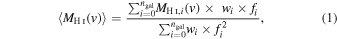
where ngal is the number of coadded spectra, and fi
and wi
are the average primary beam transmission and the weight assigned to each source. In the standard unweighted case, wi
= 1 and ∑i
wi
= ngal. This equation implements primary beam correction following the procedure detailed in Geréb et al. (2013). Throughout the paper, we assume the Fabello et al. (2011) weighting scheme ( ). The 1σ noise uncertainty (in units MH I) is evaluated by computing the rms of the noisy channels σrms of the stacked spectrum, i.e., those channels outside the spectral interval integrated to compute MH I.
To further confirm the legitimacy of our detection, we also generate a reference spectrum obtained by stacking noise spectra (one noise spectrum per galaxy) extracted at randomized positions. The positions of the noise spectra are obtained by adding a fixed angular offset to the center of each galaxy cubelet in a random direction and defined over the same spectral range as the corresponding galaxy cubelet. The angular offset (100'') is chosen to guarantee that the reference spectrum is extracted close to the galaxy spectrum, although without overlaps. Also, we double-check that the reference spectrum of each galaxy has no overlaps with other known optical galaxies, and reject it and draw a new one if there is any overlap.
We compute the integrated signal-to-noise ratio (S/N) of the final stacked spectrum as

where 〈Si 〉 is the stacked spectrum and Nch is the number of channels over which the integration is performed (e.g., Healy et al. 2019). We estimate uncertainties on the stacked spectrum by applying jackknife resampling to the galaxy sample, eliminating one galaxy at a time.
We address the problem of flux contamination due to source confusion using detailed MeerKAT-like simulated data cubes. In particular, we use the Obreschkow & Meyer (2014) flux-limited mock galaxy catalog, based on the SKA Simulated Skies semianalytic simulations (S3-SAX) to inject galaxies with realistic H i masses and clustering into a blank synthetic data cube matching the same angular and spectral size as our observations (see also Elson et al. 2016, 2019). Then, following Elson et al. (2016), we decomposed the spectrum extracted for each target galaxy into contributions from the actual target and contributions from nearby contaminating galaxies. In this way, we could accurately calculate that the level of contamination is ≲10% in all the studied cases and subtract a fixed 10% contribution from the output 〈MH I〉 from stacking.
5. Results and Discussion
In this section we present the main results of this paper. We first discuss the results yielded by stacking in the 0.23 < z < 0.49 redshift range and then compare them with known scaling relations at mean redshift z ∼ 0.
5.1. Stacking at 0.23 < z < 0.49 on MIGHTEE-H i Data
We first produce a global stack using the full galaxy sample. Figure 2 shows the resulting stacked spectrum. As anticipated, we detect the signal at ≳5σ. This represents the strongest detection obtained to date with stacking in this redshift interval. The corresponding 〈MH I〉 measurement and integrated S/N are reported in Figure 2.

Figure 2. Stacked MH I spectrum obtained in the full 0.23 < z < 0.49 redshift range we investigate in this paper. The blue solid line and the blue shaded region show the stacked spectrum and the associated jackknife uncertainties, respectively. The orange solid line and the gray shaded area indicate the reference spectrum (see text) and σrms, respectively. The red dashed and dashed‒dotted horizontal lines mark the 3σrms and 5σrms noise levels, respectively. The green vertical line shows the velocity integration limits in the MH I computation.
Download figure:
Standard image High-resolution imageIn Figure 3 we present the stacked spectra obtained in bins of M* (top row), SFR (mid row), and specific star formation rate (sSFR) (bottom row). Here, we fix empirically the bin limits to find a compromise between having enough sources per bin to claim a detection and dissecting the  in meaningful intervals. Our scaling relations are evaluated at the median redshift of our sample zmed ∼ 0.37 (see Figure 1, right panel, for the redshift distribution of our sample). To address the potential impact of the fact that the redshift distributions of the subsamples defined in different galaxy properties bins may peak at redshifts higher/lower than z ∼ 0.37 due to selection effects, we compute the median redshift of each subsample obtained with the aforementioned property cuts. The results we obtain are
- 1.M* bins: zmed = {0.36, 0.37, 0.36};
- 2.SFR bins: zmed = {0.35, 0.37, 0.38};
- 3.sSFR bins: zmed = {0.36, 0.36, 0.38}.
We notice that galaxies in all the bins have distribution peaking around the global median redshift zmed,tot ∼ 0.37, with maximum percentage deviation  , i.e., a negligible effect. As a result, we regard our results not to be affected by redshift biases.
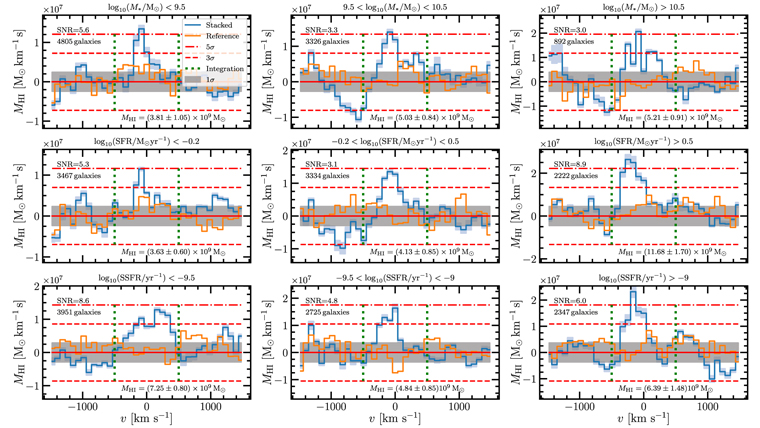
Figure 3. Stacked MH I spectra obtained in different intervals of M* (top row), SFR (mid row), and sSFR (bottom row). The title of each panel indicates the corresponding interval of galaxy properties. Lines and colors follow the same scheme as Figure 2.
Download figure:
Standard image High-resolution imageIn this case, we detect signal at ≳5σ in six bins and at ≳3σ in the remaining three bins. The corresponding 〈MH I〉 measurements are reported inside the panels in Figure 3 together with the resulting integrated S/N and the number of coadded spectra. We notice that some stacks present nonnegligible negative mass structures at ∣v∣ > 500 km s−1, where only random noise should be present. The origin of these features may be due to continuum oversubtraction or residual RFI. To test the possible effect of RFI, we repeated the stacking procedure after carefully flagging the frequency bands affected by RFI (B. Frank et al. 2022, in preparation.) and conservatively excluding the galaxies lying in such regions. This is done to mitigate the possible negative impact of badly behaved spectra, whose importance was not already suppressed by the weighting scheme. After this operation, the resulting stacked spectra no longer present outlier negative mass structures, and the MH I estimates are in excellent agreement with the ones obtained with the full sample, indicating that our results are not biased by this issue.
To fully account for these features, in the three worst cases (central and right panels in the top row, central panel in the central row of Figure 3) we include an additional uncertainty term in Equation 2, replacing σrms with σ = σrms + σdip. We estimate σdip empirically in such a way as to reduce the statistical significance of the negative structures below the detection threshold (conservatively set at 2.5σ). The final S/N shown in Figure 3 is the conservative estimate obtained after this additional operation, while previously the calculation based only on σrms returned S/N > 5 in all three cases.
5.2. Scaling Relations at z ∼ 0
We adopt as fiducial observational results at z ∼ 0 the findings presented in Guo et al. (2021, G21 hereafter). Therein, the authors investigate the interdependence of MH I, M*, and SFR, among others, performing spectral stacking on cross-matched ALFALFA (Haynes et al. 2018) and Sloan Digital Sky Survey (SDSS, York et al. 2000) data. Results are in close agreement with previous results (e.g., Brown et al. 2017; Catinella et al. 2018), where applicable. Furthermore, the scaling relations are assessed separately for star-forming and quenched galaxies. Therefore, within this work we make comparisons only with the star-forming galaxy results.
5.3. simba: Reference Cosmological Hydro Simulation
simba is a cosmological hydrodynamic simulation run with the GIZMO meshless finite-mass hydrodynamics, employing Ndm = 10243 dark matter particles and Ngas = 10243 gas elements in a  comoving volume. The simba fiducial model adopts and updates star formation and feedback subgrid prescriptions used in the mufasa simulation (Davé et al. 2016) and introduces the treatment of black hole growth and accretion from cold and hot gas. Moreover, models for on-the-fly dust production, growth, and destruction, and H i and H2 abundance computation are implemented (see Davé et al. 2019 and references therein for details).
In this work, we make use of simba galaxy catalogs at z = 0 and z = 0.4 and select only star-forming galaxies with  , consistent with our observational data, by separating the star-forming and quenched populations in the M*‒SFR plane. In particular, we flag as star-forming those galaxies with
  and
and  at z = 0 and z = 0.4, respectively. These equations are obtained from a 3σ cut below the Speagle et al. (2014) parameterizations at the corresponding redshifts, slightly modified to account for the mismatch between the simba and the observed main sequence and to separate well star-forming and quiescent galaxies.
5.4. Comparison of Scaling Relations
Figure 4 shows a comparison between our resulting scaling relations at 0.23 < z < 0.49, the findings of G21 at z ∼ 0 and the theoretical results obtained by the simba simulation at z = 0 and z = 0.4. The top-left panel shows the  relation, the top-right panel shows the
  relation, the bottom-left panel shows the
  relation, and the bottom-right panel shows the
  relation. The simba curves were generated by breaking the full galaxy sample into bins of M* (top-left panel), or SFR (bottom-left panel), or sSFR (bottom-right panel), and computing the average and standard deviation in each bin.

Figure 4. Star-forming galaxy H i scaling relations:  (top left),
  (top right),
  (bottom left), and
  . Our H i-stacking results at median redshift z ∼ 0.37 are displayed as red squares. Uncertainties on red squares along the x-axis, not shown for the sake of clarity of visualization, correspond to the width of the bins. The red dashed line represents the fit to our data. Our reference results at z ∼ 0 (G21, Guo et al. 2021) are plotted as a blue solid line. Green dotted and yellow dashed‒dotted lines show the predictions of the simba cosmological hydrodynamic simulation at z = 0 and z = 0.4, respectively, for comparison. Shaded regions indicate 1σ uncertainties.
Download figure:
Standard image High-resolution imageWe fit a linear model  to our data at z ∼ 0.37. We compute the mean values for the fitting parameters and the associated uncertainties (68% confidence interval) through parametric bootstrap resampling of our data, drawing 10,000 samples and fitting the model with a least-squares minimization to each sample. The resulting best-fitting coefficients are
- 1.
 : (∼4.8σ difference from z ∼ 0),
- 2.: ,
- 3.: ,
- 4.: , .


The  relation (Figure 4, top-left panel) is found to have comparable normalization at the two redshifts at
  , but different slopes, the relation at z = 0 has a steeper slope than that at z ∼ 0.37. In particular, low-M* galaxies (
 ) are ∼0.5 dex more HI-rich at z ∼ 0.37 than at z ∼ 0, while massive galaxies (
 ) at z ∼ 0.37 and z ∼ 0 converge to similar MH I values within 0.25 dex (and compatible within uncertainties). The same result can be visualized in terms of the H i fraction in the
  plane (Figure 4, top-right panel).
In terms of star formation properties, the SFR displays a weaker correlation with MH I than at z ∼ 0 (bottom-left panel). Galaxies having  show no MH I evolution. Instead, galaxies at z ∼ 0 with
  feature an excess in MH I of up to ∼0.5 dex in
  ) at fixed
  with respect to galaxies at z ∼ 0.37. Lastly, the fH I–sSFR relations at z ∼ 0 and z ∼ 0.37 converge at
  , while the galaxies at z ∼ 0.37 at (fixed) larger sSFR have systematically smaller fH I than at z ∼ 0 (up to ∼0.8 dex).
5.5. Discussion
Our findings suggest evidence for moderate evolution of scaling relations from z ∼ 0.37 to z ∼ 0. Low-M* galaxies have depleted their H i reservoirs over the last 4 Gyr. The long H i depletion time due to star formation for these galaxies,  , suggests that star formation depletes only ΔMH I ∼ 1 × 10⁹
M⊙ (i.e., ∼0.15 dex) over the last 4 Gyr. As a result, we argue that star formation alone could not be able to account for the observed reduction in MH I from z ∼ 0.37 to z ∼ 0 and that another H i depletion/removal mechanism may be acting in parallel to star formation. On the other hand, massive galaxies have experienced an efficient replenishment of the H i content in their disks, counteracting the H i depletion due to star formation and feedback processes. In particular, assuming the H2 formation rate and the SFR are in equilibrium, and that the H2 depletion time
, suggests that star formation depletes only ΔMH I ∼ 1 × 10⁹
M⊙ (i.e., ∼0.15 dex) over the last 4 Gyr. As a result, we argue that star formation alone could not be able to account for the observed reduction in MH I from z ∼ 0.37 to z ∼ 0 and that another H i depletion/removal mechanism may be acting in parallel to star formation. On the other hand, massive galaxies have experienced an efficient replenishment of the H i content in their disks, counteracting the H i depletion due to star formation and feedback processes. In particular, assuming the H2 formation rate and the SFR are in equilibrium, and that the H2 depletion time  at z < 0.5 is of order
  (e.g., Tacconi et al. 2018 and references therein), there must be an efficient H i accretion mechanism fueling massive galaxies (see, e.g., Sancisi et al. 2008). This is also consistent with the H i depletion time of massive galaxies that we are able to derive in this work:
  . The nature of the H i growth into galaxies is still debated, with coplanar accretion from cosmic flows being favored by observations of Mg ii absorbers in quasars down to z ∼ 0.2 and statistical arguments (e.g., Bouché et al. 2013; Peng & Renzini 2020, and references therein). Theoretical predictions indicate that at z < 0.5, the main cold gas accretion mode onto galaxies is not cosmological accretion (as suggested for accretion at high z by results based on observations; e.g., Conselice et al. 2013) or the galactic fountain mechanisms (e.g., Fraternali 2017), but mergers (e.g., Sánchez Almeida et al. 2014; Padmanabhan & Loeb 2020). Furthermore, simulations tell that most of the H i in the universe is already contained in galaxy disks at the probed redshifts (e.g., ∼97% at z = 0 in Villaescusa-Navarro et al. 2018), thus making mergers a potential efficient H i transfer mechanism. We speculate that minor mergers between low-M* H i-rich galaxies and massive galaxies could be the mechanism that mainly refills the latter of H i. Intriguingly, Jackson et al. (2022) recently found evidence in observations that minor mergers play a major role in the formation of H i-rich massive disk galaxies at z ∼ 0, supporting our proposed scenario. On the other hand, Di Teodoro & Fraternali (2014) argue that cold gas transfer through minor mergers at z ∼ 0 is not able to sustain star formation, even under stringent assumptions. This is however not in direct contrast with our findings, as low-M* galaxies are found to contain much less H i at z ∼ 0 than at z ∼ 0.37. In any case, our conclusions do not exclude the scenario in which smooth accretion from the intergalactic medium is the dominant cold gas accretion onto galaxies.
The decrease in MH I observed in highly star-forming galaxies with  from z ∼ 0.37 to z ∼ 0 suggests that H i features a stronger correlation with star formation at the latter redshift. Interesting insights are offered by the fH I–sSFR relation. In fact, making bins in sSFR corresponds to binning the SFR−M* plane (central panel, Figure 1) with bin limits being diagonal lines in the
  plane. In particular, the three bins roughly correspond to galaxies in the lower (and below), central, and upper (and above) parts of the main sequence, from lower to higher sSFR, respectively. This suggests that the galaxies at fixed sSFR lying above the main sequence are the ones experiencing a larger increase of their fH I over the last ∼5 Gyr.
To develop a more complete picture on the SFR evolution, we would need to include also the H2 scaling relations in our framework, which goes, however, beyond the scope of the paper. We leave such a study for future work.
However, we notice that H i replenishment in massive galaxies is not able to supply enough gas to fully sustain star formation and, hence, prevent the observed reduction in the SFR. We speculate that the main reason for this could be that fresh H i accretes onto the outer part of the disk and takes a significant amount of time to migrate toward the region within the optical radius—where the bulk of star formation takes place—due to galaxy angular momentum (Peng & Renzini 2020).
Interestingly, our findings are in good agreement with the predictions of the simba simulation employing the full baryon physics model. The only significant discrepancy is found in the  plane and is due to the simba main sequence at z = 0.4 having a systematic positive SFR offset with respect to the observed main sequence (both the Speagle et al. 2014 parameterization and, even more, the observed sample), especially at large M*. The immediate aim of this comparison is to provide a minimum contextualization of our observational results into a theoretical scenario. However, the agreement between theory and observations offers the unique advantage of being able to use simba as a benchmark to study which is the driving process that determines the observed scaling relations, and to compare it more thoroughly to our data to better constrain models. This goes beyond the scope of the paper, and we leave it for future work. The full simba suite also includes other runs with only partial modeling of feedback and baryon processes. Davé et al. (2020) find that the most crucial phenomena to be modeled to reproduce the high-mass end of the H i (and H2) mass function are AGN, X-ray, and jet feedback. We plan to perform an in-depth investigation of the impact of these aspects on scaling relations in forthcoming publications, comparing our findings with other cosmological simulations and semianalytical models too.
6. Conclusions
In this paper, we have performed stacking of 9023 21 cm undetected star-forming galaxy spectra extracted from MIGHTEE-H i data cubes at 0.23 < z < 0.49 in the COSMOS field. In particular, we have subdivided the full sample into galaxy properties subsets with the aim of directly measuring for the first time H i scaling relations at a median redshift zmed ∼ 0.37.
We find moderate evolution of the probed scaling relations from z ∼ 0.37 to z ∼ 0, with no significant evolution in the  and
and  relations at
  , implying the necessity of an efficient H i replenishment mechanism in massive galaxies. The
  and
and  relations evidence how highly star-forming galaxies evolve significantly in SFR (sSFR) at fixed MH I (fH I), while the evolution of scaling relations at lower SFR (sSFR) is milder. We argue that the aforementioned H i replenishment mechanism is not able to prevent star formation quenching in massive galaxies. We will further investigate these aspects in forthcoming publications.
We argue that future MIGHTEE-H i data beyond the Early Science data set will allow us to strengthen the statistical significance of the results, as they will enlarge the footprint at 0.23 < z < 0.49 from the ∼1.5 deg2 of the COSMOS field used in this paper, to ∼20 deg2 of the final data release.
The authors warmly thank the anonymous referee for the constructive review and helpful comments they offered. The authors also thank Alvio Renzini for insightful comments and discussions. F.S. acknowledges the support of the doctoral grant funded by the University of Padova and by the Italian Ministry of Education, University and Research (MIUR). G.R. acknowledges the support from grant PRIN MIUR 2017-20173ML3WW_001. M.V. acknowledges financial support from the South African Department of Science and Innovation's National Research Foundation under the ISARP RADIOSKY2020 Joint Research Scheme (DSI-NRF grant No. 113121) and the CSUR HIPPO Project (DSI-NRF grant No. 121291). N.M. acknowledges support of the LMU Faculty of Physics. H.P. acknowledges support from the South African Radio Astronomy Observatory (SARAO). S.H.A.R. is supported by the South African Research Chairs Initiative of the Department of Science and Technology and National Research Foundation. C.F. is the recipient of an Australian Research Council Future Fellowship (project number FT210100168) funded by the Australian Government. A.A.P. acknowledges support of the STFC consolidated grant ST/S000488/1 and from the Oxford Hintze Centre for Astrophysical Surveys, which is funded through generous support from the Hintze Family Charitable Foundation. I.P. acknowledges financial support from the Italian Ministry of Foreign Affairs and International Cooperation (MAECI grant No. ZA18GR02) and the South African Department of Science and Technology's National Research Foundation (DST-NRF grant No. 113121) as part of the ISARP RADIOSKY2020 Joint Research Scheme. J.M.v.d.H. acknowledges support from the European Research Council under the European Unions Seventh Framework Programme (FP/2007-2013) / ERC grant Agreement nr. 291531 (HIStoryNU). The MeerKAT telescope is operated by the South African Radio Astronomy Observatory, which is a facility of the National Research Foundation, an agency of the Department of Science and Innovation. We acknowledge the use of the ilifu cloud computing facility—www.ilifu.ac.za, a partnership between the University of Cape Town, the University of the Western Cape, the University of Stellenbosch, Sol Plaatje University, the Cape Peninsula University of Technology, and the South African Radio Astronomy Observatory. The Ilifu facility is supported by contributions from the Inter-University Institute for Data Intensive Astronomy (IDIA a partnership between the University of Cape Town, the University of Pretoria, the University of the Western Cape and the South African Radio Astronomy Observatory), the Computational Biology division at UCT and the Data Intensive Research Initiative of South Africa (DIRISA).
Footnotes
- *
Released on July 29, 2022.
- 30
Outliers are defined as those galaxies having ∣zspec − zphot∣ > 0.15 × (1 + zspec).