
Optimization of Thermal Backfill Configurations for Desired High-Voltage Power Cables Ampacity


1
Faculty of Electrical and Control Engineering, Gdańsk University of Technology, Narutowicza 11/12, 80-233 Gdańsk, Poland
2
Research and Development Centre, Eltel Networks Energetyka SA, Gutkowo 81D, 11-041 Olsztyn, Poland
*
Author to whom correspondence should be addressed.
Energies 2021, 14(5), 1452; https://doi.org/10.3390/en14051452
Submission received: 28 January 2021
/
Revised: 19 February 2021
/
Accepted: 3 March 2021
/
Published: 7 March 2021
(This article belongs to the Special Issue MV and HV Transmission Lines)
Abstract
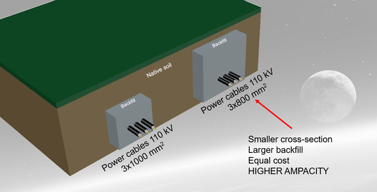
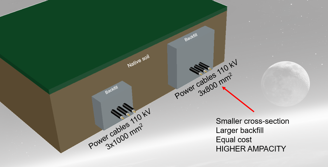
:The ampacity of high-voltage power cables depends, among others, on their core cross-sectional area as well as thermal resistivity of the thermal backfill surrounding the cables. The cross-sectional area of the power cables’ core is selected according to the expected power to be transferred via the cable system. Usually, the higher the power transfer required, the higher the cross-sectional area of the core. However, the cost of high-voltage power cables is relatively high and strictly depends on the dimensions of the core. Therefore, from the economic point of view, it is interesting to focus on the improvement of the thermal condition around the cables, by changing the dimension of the thermal backfill, instead of increasing the power cables’ core cross-sectional area. In practice, it is important to find the optimal dimensions of both cable core and thermal backfill to achieve the economically attractive solution of the power cable transfer system. This paper presents a mathematical approach to the power-cable system design, which enables selecting the cost-optimal cross-section of a power cable core depending on the dimensions of the thermal backfill. The proposal herein allows us to indicate the condition in which it is advantageous to increase the core cross-sectional area or to expand the dimension of the backfill. In this approach, the optimal backfill geometry can also be evaluated. The investment costs of the 110 kV power cable system with the core cross-sectional areas consecutively equal to 630, 800 and 1000 mm2 have been compared.
1. Introduction
The ampacity of the power cables mainly relies on the cross-sectional area of the power cable cores. The higher the required ampacity, the higher the required cross-sectional area of the cable core. To ensure the ampacity specified by the investor, designers have to evaluate required parameters of a cable, especially its appropriate core cross-section, based on the guidelines included in the IEC 60287 standards series, primarily in IEC 60287-1-1 [1]. Usually, the cross-sectional area of the cable core is selected to be as low as possible because each subsequent cable size increases its cost—by 15÷40% for 110 kV cables analyzed in this article. To keep the cross-sectional area of the cable unchanged, it is possible to increase the ampacity by creating favorable thermal conditions around the buried cables. Such favorable conditions may be achieved by the application of the thermal backfill of relevant geometry and relatively low thermal resistivity. The backfill is assumed to be a medium with known heat dissipation properties, usually better than native soil, which counteracts the influence of seasonal weather changes. The backfill has known properties at various temperatures. Therefore, the heat transfer from the cables is easy to evaluate for expected operating temperatures. The use of backfill also reduces the risk of damage to the cable due to sharp-edged stones which would be included in native soil near the cable.
The issue of the calculation of the power cables’ ampacity and, hence, the selection of their cores’ cross-sectional areas is considered in many works and papers. As the official historical start of calculating cable ampacity, the society of technicians and engineers recognizes Kennelly’s conference paper “Heating Conductors by Electric Currents” from 1889 [2]. Overall, Kennelly’s work led to the formulation of the image method, which allowed the analytical calculation of the temperature at any point of the soil [3]. Most important works on the subject were recognized and collected by Anders [4,5]. The study of the literature regarding topics closest to the topic focused on by the authors shows that a significant number of papers consider only technical aspects of power cable lines design. The papers [6,7,8] refer to the buried power cables and searching for their ampacity for various cables configurations in the ground. The effect of the dry zone around the cables on their ampacity is studied in the papers [9,10]. Such an issue is also considered in [11] when dynamic management of the cable system is applied. Thermal phenomenon and ampacity of power cables installed in pipes are analyzed in the work [12]. A similar analysis, but refereeing to the cables in ducts, is presented in papers [13,14]. The ampacity of a tunnel cable is studied in [15], whereas the ampacity of insolated power cables and the risk of their overheating is investigated in [16]. However, taking into account the particular investment, it is necessary to pay attention to the economic aspects as well. Such a consideration, in some cases, may modify previously assumed technical solutions. In the paper [17], as well as in [18,19], methods of optimizing cable installation costs are presented, developing the Neher–McGrath approach [20] with installation cost factors influencing the optimal cross-section of the backfill for a given load capacity and vice versa (by specifying the cost of the project). According to this approach, it is possible to calculate ampacity, which will be achieved by investing in various elements of the system (including the thermal backfill). Some subsequent works have developed this issue and a good summary is presented in the paper [21]. In the research work [22], Cichy et al. present detailed costs of materials of the high-voltage cable line and the economic return during its operation. Most of the distribution system operators (DSOs), especially in Poland, do not pay attention to the power losses in cables, which depend on the cross-section of the core. Therefore, they tend to minimize the investment costs, which is strictly related to selecting a cable having cross-sectional area of the core as low as possible. The PhD thesis in [23] presents the investment profitability curve depending on the lifetime of a cable line, indicating that the smaller the length and/or cross-section of the core, the disproportionately greater the expenditure incurred by heat losses.
In this paper, the authors propose a method which automates and accelerates the calculation of the power cables’ ampacity taking into account economic aspects. Based on the authors’ proposal, it is possible to indicate the desired ampacity of cables when one has strict economic boundary conditions. According to the assumption presented by the authors, the cost-optimal cross-section of a power cable core depending on the dimensions of the thermal backfill can be evaluated. The proposal also enables indicating the condition in which it is advantageous to increase the core cross-sectional area or to expand the dimension of the backfill. This paper is an extension of the considerations referred to in the optimization problem posed by El-Kady [17] and examined by Anders [19]. This work is also complementary to the papers [24,25,26], considering an economic aspect of the power cable line design. Analyzing other works, this work is enriched with the selection of thermal backfill geometry and the evaluation of the average costs of design of power cable lines in Poland. It is worth mentioning that, according to standard IEC 60287-3-1 [27] and the surveys of the CIGRE B1.41 [28] group respondents, each country has its assumptions in terms of the reference temperature of the ground, its overall thermal resistance and the cost of laying the cable line. It influences the total cost and performance of the cable line in a considered country.
2. Theoretical Background
Evaluation of the power cables ampacity is usually performed according to the multipart standard IEC 60287 “Electric Cables–Calculation of the Current Rating”. For example, based on [1], the ampacity of a single cable directly buried in the ground, where drying out the soil is excluded, can be calculated according to the following expression:
where:
IAMP is the ampacity of a cable in ground, A;
Δθ is the permissible temperature rise of the conductor (core) above ambient temperature, K;
Wd is the dielectric losses per phase, W/m;
T1 is thermal resistance (per core) between the conductor and sheath/insulation, (K·m)/W;
T2 is the thermal resistance between the sheath/insulation and armor, (K·m)/W;
T3 is the thermal resistance of external serving of the cable, (K·m)/W;
T4 is the external thermal resistance of the surrounding medium, (soil/backfill), (K·m)/W;
nco is the number of conductors in a power cable;
Rco is the AC resistance of a conductor (core) at its permissible temperature, Ω/m;
γco is the conductivity of a conductor (core) at its permissible temperature, m/(Ω/mm2);
sco is the cross-sectional area of a conductor (core), mm2;
λ1 is the ratio of the total losses in metallic sheaths (if any) to the total conductor losses;
λ2 is the ratio of the total losses in metallic armor (if any) to the total conductor losses.
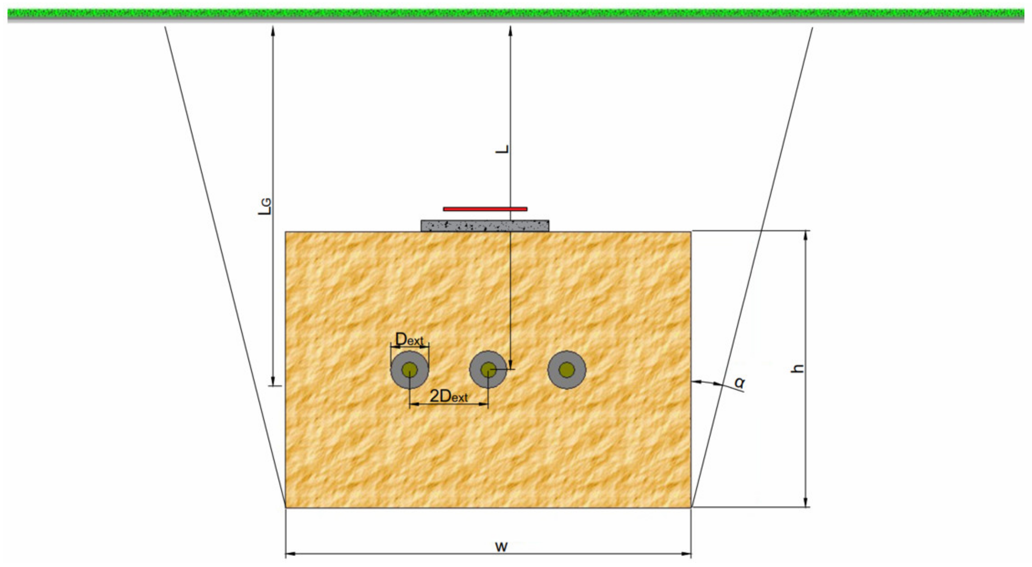
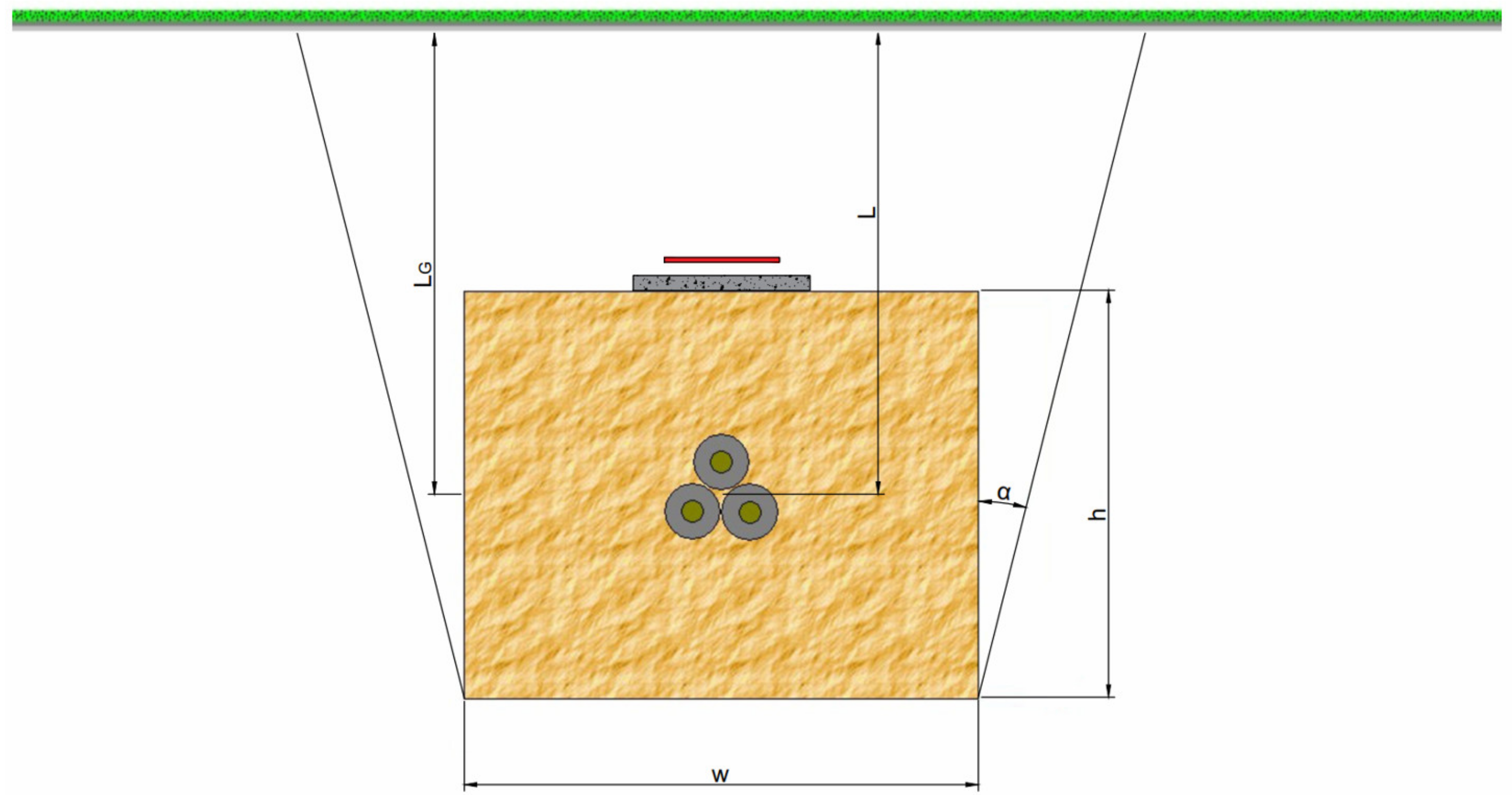
Analysis of the expression (1) leads to the conclusion that cables’ ampacity is dependent, among other factors, on the thermal resistance T4 of the medium surrounding the power cables. Hence, the increase in the ampacity can be done by creating a favorable heat transfer from the surface of cables to the ground. The favorable heat transfer from cables is usually ensured by replacing the native soil with the thermal backfill of relatively low thermal resistivity—less than 1.0 (K·m)/W. Figure 1 shows a typical arrangement of the cable line in a flat formation when thermal backfill of width w and height h is used. The presented arrangement reflects real cables placement—it includes a backfill, pavement slabs (grey rectangular element) for the protection against mechanical damage, and a warning tape (red line). The modeled geometry for the trefoil formation is presented in Figure 2.
External thermal resistance T4 of the uniform single cable surrounding can be written according to the Kennelly’s theorem [29] as:
where:
Dext is the external diameter of the cable, mm;
L is the distance from the ground surface to the cable center, mm;
ρe is the thermal resistivity of the native soil, (K·m)/W.
For a high value of the ratio 2L/Dext (more than 10) the aforementioned relation (2) can be simplified to the following expression:
When cables are placed in the thermal backfill of thermal resistivity ρc and thermal resistivity of the surrounding native soil is equal to ρe, based on the provisions of the standard IEC 60287-2-1 [30], the correction factor T4corr to the thermal resistance should be calculated as follows:
where:
LG is the distance from the ground surface to the center of the backfill, mm;
N is the number of loaded cables in the backfill;
rb is the equivalent radius of the backfill, mm;
ρe is the thermal resistivity of the native soil, (K·m)/W;
ρc is the thermal resistivity of the backfill, (K·m)/W.
The thermal backfill has usually a rectangular cross-section but the heat transfer is conducted radially. Therefore, based on [29], it is necessary to convert the rectangular dimensions of the backfill to the equivalent radius rb:
where: x = min(w, h) and y = max(w, h).
Equation (5) is valid when the ratio x/y takes values: 0.33 < x/y < 3. For other values of the x/y ratio, evaluation of the equivalent radius rb with (5) gives inaccurate values—in such cases data from tables included in [19] (p. 233) can be used.
Based on (3) and (4), the corrected thermal resistance T4* is expressed as follows:
As formula (6) shows, the coefficient T4* depends on the dimensions of the backfill. In further analysis, when the optimal dimension of the backfill is searched for, the following constraints are introduced:
Formulas (7) and (8) represent the minimum permissible depth of the cables, according to national practice/regulations [31], whereas formulas (9) and (10) take into account the minimal practicable dimensions of the backfill. The aforementioned constraints allow a consideration of the acceptable, from the practical point of view, arrangements of the cable system.
3. A Proposal of the Cable System Optimization
The total cost of the power cable lines performance can be represented (in general) by the following dependence:
where:
PK is the cable cost;
PE is the cost of the performed excavation;
PZZ is the cost of backfilling with the thermal backfill, sand and native soil as well as compaction;
PB is the backfill material cost;
PES other costs;
The values of the particular components included in (11) are dependent on the local market conditions. Table 1 presents sample unit costs referred to the cable line performance in Poland.
For the optimization purpose, the objective function related to costs can be presented in the following form (for symbols see Figure 1 and Table 1):
Particular factors included in the formula (12) are strictly correlated with the geometry of the cable systems presented in Figure 1andFigure 2.
In the optimization process, the Nelder–Mead method [32,33] is applied. This method is a common direct search method. For a function of n variables, the algorithm maintains a set of n + 1 points forming the vertices of a polytope in n-dimensional space. The algorithm selection does not take a major issue in the optimization problem as only a sixth dimension problem is faced that gives global solution from over 50,000 cases. It can be done with the use of a personal computer of average class. For a greater number of variables, there is the possibility of the genetic algorithm application, which could be more efficient.
To obtain the desired solution, the maximum of the ampacity Imax is searched for, as follows:
The purpose of the optimization is to find the best relation of the power cable line performance cost to the ampacity of the power cables. The function P forces optimal geometry of backfill regarding investment cost, dimensions h, w and LG included in (13). In consequence, one can obtain maximal ampacity of power cables with relation to the optimal geometry of the backfill.
In the optimization process, the boundary conditions expressed by Relations (7)–(10) are taken into account. All ampacity calculations were made with the assumption that:
- The ambient temperature of the ground is equal to 20 °C;
- The max permissible temperature for the cable is equal to 90 °C;
- The thermal resistivity of the backfill (cement–sand mixture) is assumed within the range ρc = 0.5–0.9 (K·m)/W;
- The angle of the excavation trench is constant (α = 15°);
- The distance L from the ground surface to the cable/cables center for particular formation (flat or trefoil) is constant (for the flat formation: L = 1200 mm + Dext/2; for the trefoil formation: L = 1200 mm + Dext/2 + Dext/√3);
- The maximum accepted price of the cable line is equal to 720 EUR/m.
4. Discussion
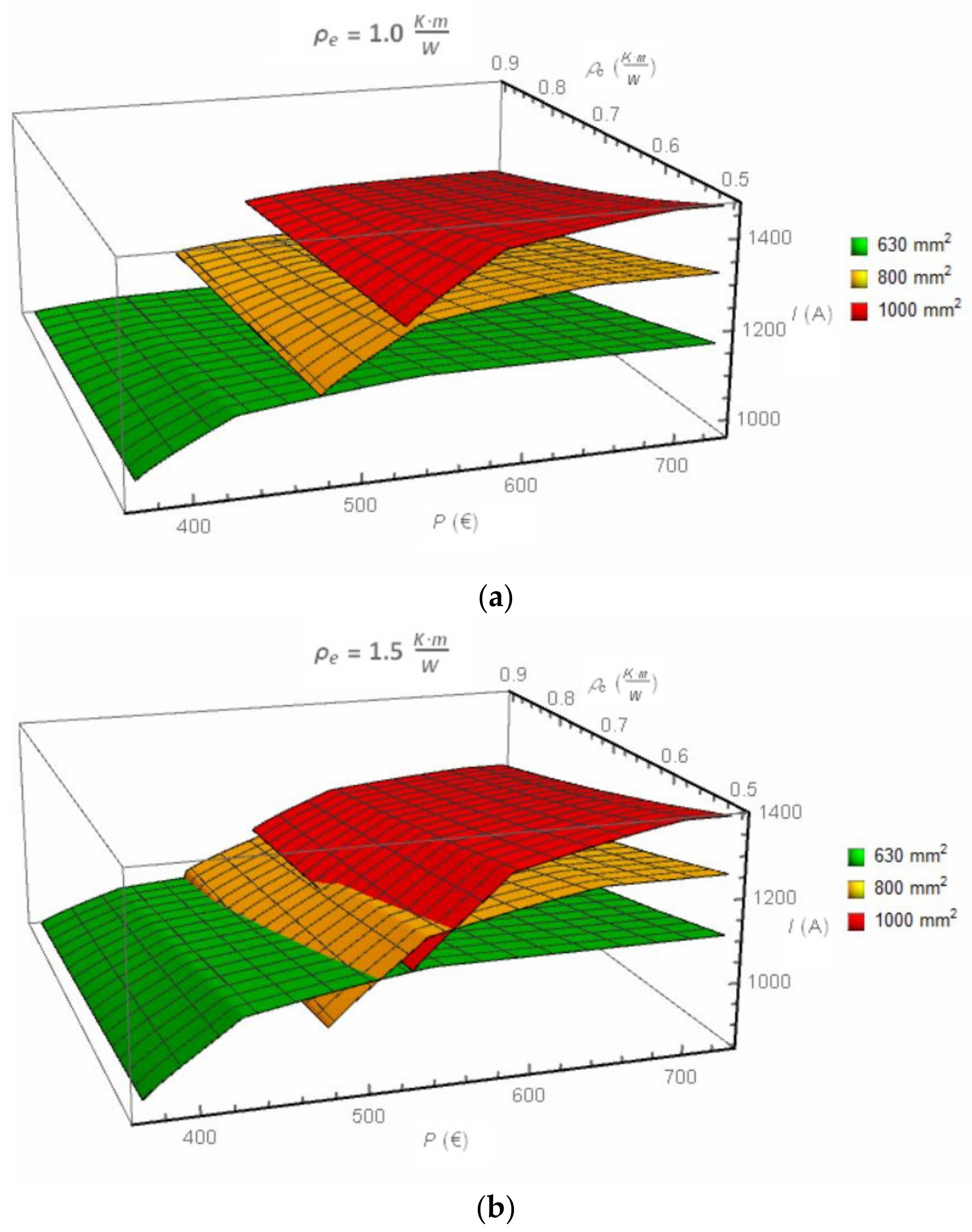
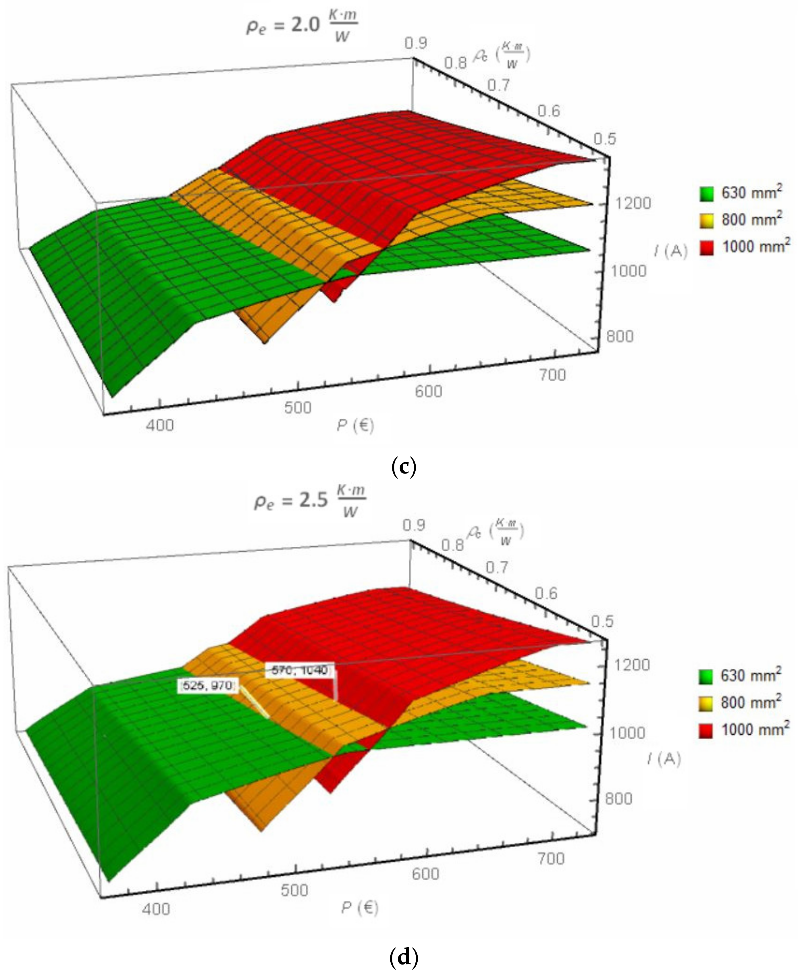
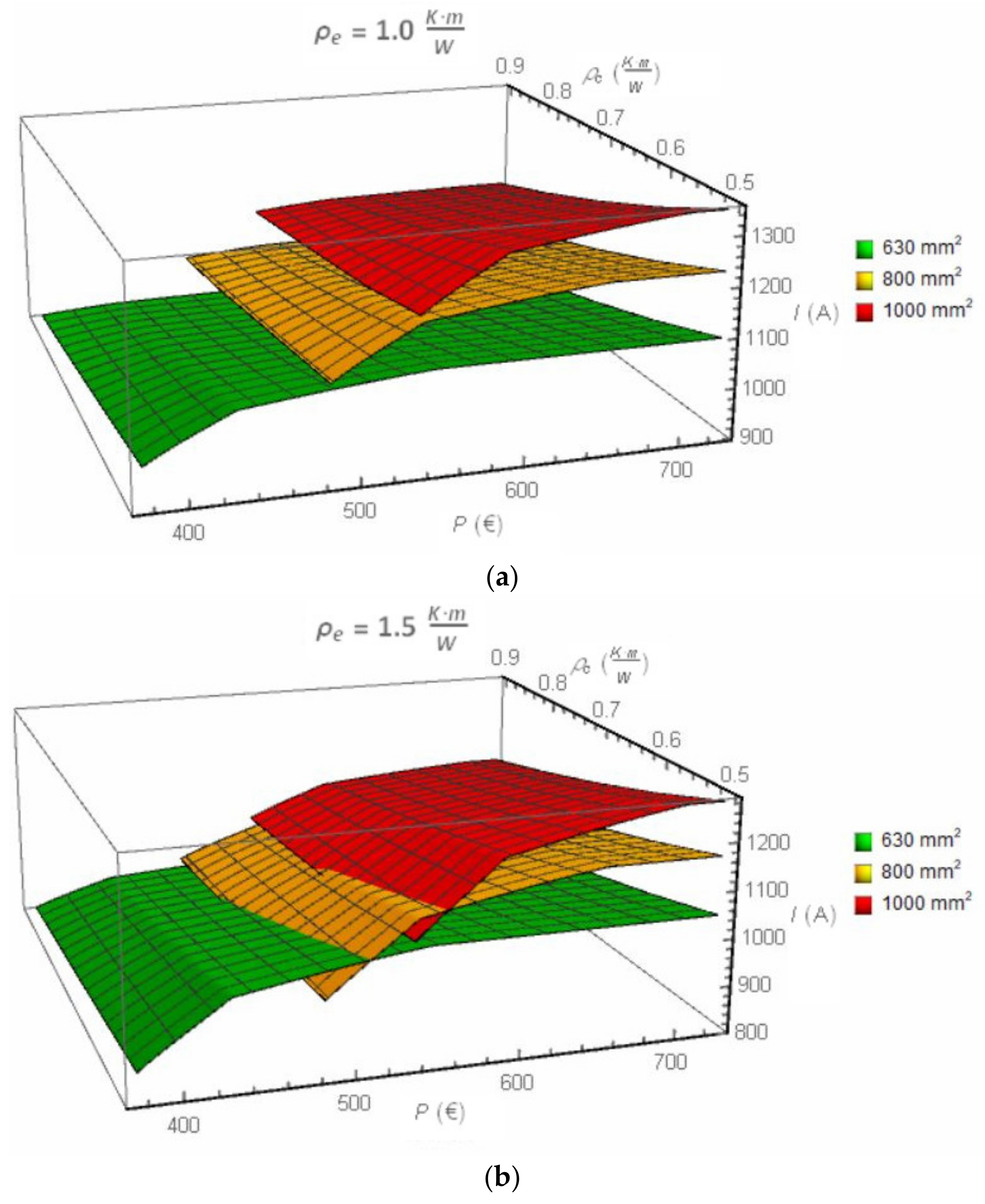
Results of the investigation are presented in Figure 3andFigure 4. Generally, as expected, the ampacity of the cable line is increasing along with increasing its cost P and decreasing thermal resistivity of the backfill ρc. However, when the difference between thermal resistivities of backfill ρc and native soil ρe increases, one can observe the intersection of planes for particular cable cross-sections—compare results for the flat formation (Figure 3a vs. Figure 3c and vs. Figure 3d) and for the trefoil formation, compare Figure 4a vs. Figure 4c and vs. Figure 4d. The planes’ intersection points indicate that a given ampacity can be obtained by various cross-sectional areas of cables. The intersection points also indicate the optimal transition to the cable of the higher cross-sectional area.
For example, for the flat formation, thermal resistivity of the native soil ρe = 2.5 (K·m)/W and thermal resistivity of the backfill ρc = 0.6 (K·m)/W (Figure 3d), the ampacity of the 630 mm2 cable starts from 700 A at the cost below EUR 400 (green plane at the left down part of the Figure 3d). Investing in cable backfill for the 630 mm2 cable increases its ampacity but in consequence, also the cost. However, it is visible that within the cost range of EUR 475–525, the green plane (630 mm2 cable) is located higher than the orange plane (800 mm2 cable). It means that the use of the 630 mm2 cable instead of 800 mm2 is more profitable because the ampacity of the 630 mm2 cable is higher than that of the 800 mm2 cable at the same cost. For the cost EUR 475, the ampacity of the 630 mm2 cable is equal to I630 = 884 A whereas the 800 mm2 cable has I800 = 771 A, which gives around a 15% difference in ampacities (the backfill of the cable line with cables 630 mm2 has a greater volume). The ampacity of two cables equalizes at point EUR 525, 970 A. This point indicates that it is better to use the 800 mm2 cable, instead of the 630 mm2 cable, if the desired ampacity is higher than 970 A.
The second characteristic point in Figure 3d is marked as (EUR 570, 1040 A). It presents the point of changing the 800 mm2 cable to the 1000 mm2 cable. If the desired ampacity is higher than 1040 A, the use of the 1000 mm2 cable is the most profitable solution. After analysis of Figure 3d, for the native soil ρe = 2.5 (K·m)/W and thermal resistivity of the backfill ρc = 0.6 (K·m)/W the conclusions are as follows:
- The 630 mm2 cable is profitable for ampacities below 970 A;
- The 800 mm2 cable is profitable for ampacities between 970 and 1040 A;
- The 1000 mm2 cable is profitable for ampacities higher than 1040.
Characteristic ampacity of 970 A can be achieved by either the 630 mm2 cable or the 800 mm2 cable, whereas the ampacity 1040 A can be achieved by either the 800 mm2 cable or the 1000 mm2 cable.
This issue can be analyzed from another point of view. If one expects the ampacity 970 A, the solution is the use of either the 630 mm2 cable or 800 mm2 with relevant backfill. It gives a cost of EUR 525. If the 1000 mm2 cable is used (for the ampacity 970 A), the unit cost of the cable line is equal to EUR 566, which is 8% more. Generally, the plane in Figure 3 located at the highest level gives the most profitable solution.
A similar example analysis of the cable line for the trefoil formation (the native soil ρe = 2.5 (K·m)/W and thermal resistivity of the backfill ρc = 0.6 (K·m)/W—Figure 4d) gives the following conclusions:
- The 630 mm2 cable is profitable for ampacities below 910 A;
- The 800 mm2 cable is profitable for ampacities between 910 and 970 A;
- The 1000 mm2 cable is profitable for ampacities higher than 970.
Characteristic ampacity 910 A can be achieved by either the 630 mm2 cable or the 800 mm2 cable, whereas the ampacity 970 A can be achieved by either the 800 mm2 cable or the 1000 mm2 cable.
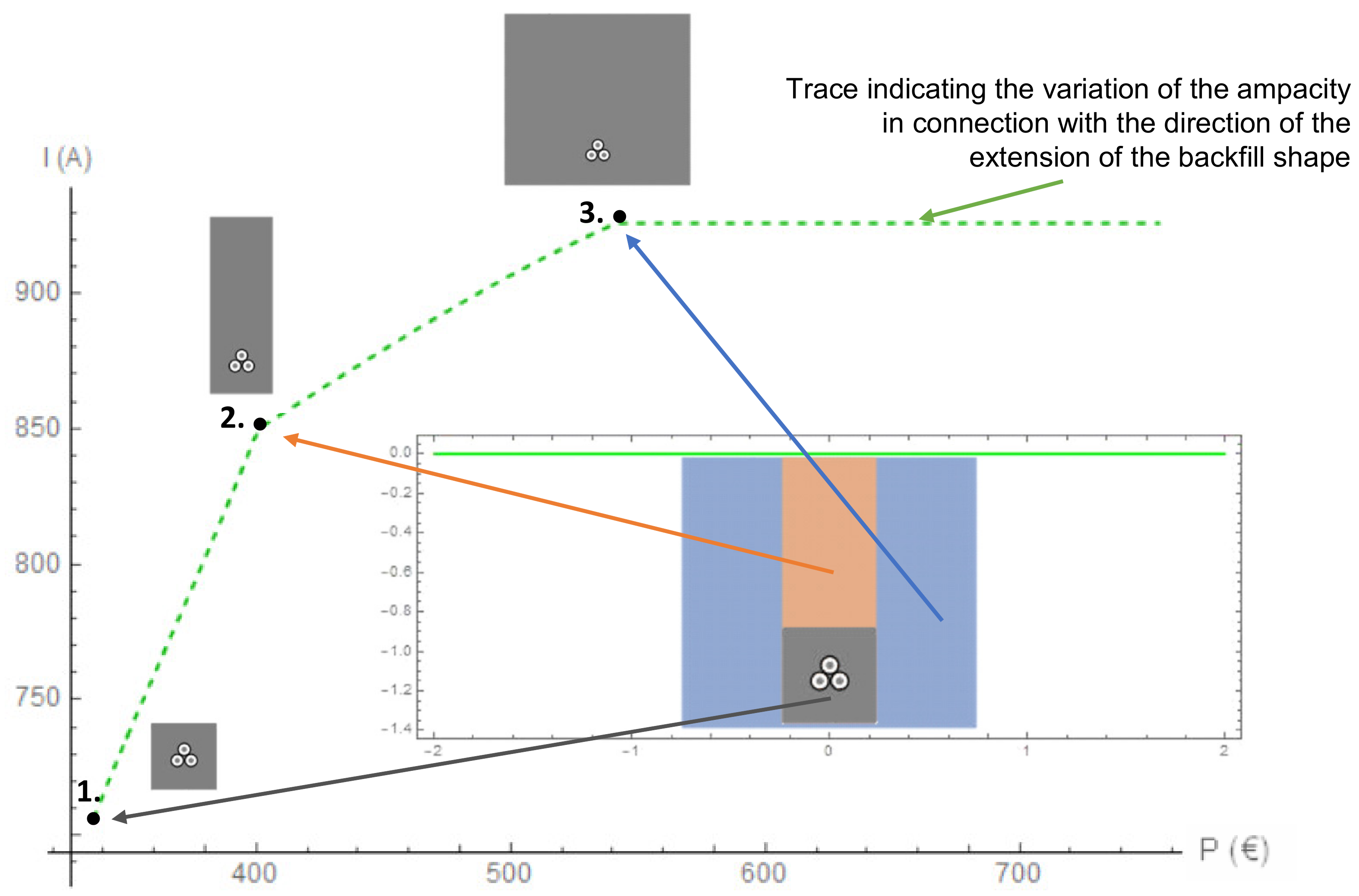
As it has been mentioned, a higher ampacity of the cables can be obtained by keeping the same cross-section of the cable core but creating relevant backfill area/volume. Figure 5 presents various backfill areas for the cable line with 630 mm2 cables laid in the trefoil formation where the native soil is ρe = 2.5 (K·m)/W and thermal resistivity of the backfill is ρc = 0.6 (K·m)/W. If the backfill area is the smallest, the ampacity is equal to 706 A (point 1 in Figure 5). For the largest possible backfill area in the considered case (point 3 in Figure 5), the ampacity is as high as 926 A. The green dashed trace indicates the variation of the ampacity as a function of cost P and the direction of the extension of the backfill shape. The shape between point 1 and point 2 has a constant width—only its height varies. It is an assumption made by the authors, based on practical applications. If the maximal height is achieved (point 2), the backfill width is increased (along the green trace between point 2 and point 3).
5. Conclusions
The desired ampacity of power cable lines can be obtained by selecting either a relatively high cross-sectional area of the power cables or modification of thermal condition around the cables, e.g., by extension of the thermal backfill area. During the project stage of the power cable lines, both the technical and economic aspects should be taken into account—such an approach leads to the optimal solution. For example, urbanized areas influence the reduction in the possible excavation area, and, hence, reduce the distance between phases which leads to lower ampacity. In consequence, the expansion of the backfill area is not a possible solution. The same conclusion is valid if a low difference between thermal resistivity of the native soil and the backfill occurs—the enlargement of the backfill area is not profitable. In such cases, the only cost-effective way of increasing the ampacity is to increase the cable cross-section. However, when the difference between the aforementioned thermal resistivities is high, e.g., the native soil has ρe = 2.5 (K·m)/W and the backfill has ρc = 0.6 (K·m)/W, the cost-effective transition point of cable cross-section is observed, meaning that the given cost enables to achieve various ampacities of the cable line depending on which cross-section of the cable and shape of the backfill area are applied. For example, if the assumed cost is EUR 475, the ampacity of the 630 mm2 cable (with large backfill area) can be higher by 15% than the ampacity of the 800 mm2 cable. Thus, in some cases, it is more beneficial to invest in the thermal backfill rather than in the high cross-sectional area of the cables.
The approach presented by the authors, related to the power-cable system’s design, can be interesting and useful for investors as well as power cable line designers to optimize the high-voltage power cable systems. Based on the proposal, the authors are considering the development of an easy-to-use computer tool for supporting cable line designers.
Author Contributions
Conceptualization, S.C. and F.R.; methodology, F.R.; software, F.R.; validation, S.C., formal analysis, S.C.; investigation, S.C. and F.R.; resources, S.C. and F.R.; writing—original draft preparation, S.C. and F.R.; writing—review and editing, S.C.; visualization, F.R.; supervision, S.C. All authors have read and agreed to the published version of the manuscript.
Funding
This research was supported by Gdańsk University of Technology as well as Ministry of Education and Science.
Conflicts of Interest
The authors declare no conflict of interest.
References
- International Electrotechnical Commission. Electric Cables–Calculation of the Current Rating–Part 1–1: Current Rating Equations (100% Load Factor) and Calculation of Losses–General; International Electrotechnical Commission: Geneva, Switzerland, 2001. [Google Scholar]
- Kennelly, A.E. Heating Conductors by Electric Currents; Association Edison Ilium: Niagara Falls, NY, USA, 1889; pp. 11–32. [Google Scholar]
- Enescu, D.; Colella, P.; Russo, A. Thermal assessment of power cables and impacts on cable current rating: An overview. Energies 2020, 13, 5319. [Google Scholar] [CrossRef]
- Anders, G.; El-Kady, M. Transient ratings of buried power cables. I. Historical perspective and mathematical model. IEEE Trans. Power Deliv. 1992, 7, 1724–1734. [Google Scholar] [CrossRef]
- Holyk, C.; Anders, G. Power cable rating calculations—A historical perspective [History]. IEEE Ind. Appl. Mag. 2015, 21, 6–64. [Google Scholar] [CrossRef]
- De Leon, F. Calculation of Underground Cable Ampacity; CYME Int. TD: St. Bruno, QC, Canada, 2005. [Google Scholar]
- De Mey, G.; Xynis, P.; Papagiannopoulos, I.; Chatziathanasiou, V.; Exizidis, L.; Więcek, B. Optimal position of buried power cables. Elektron. Elektrotechnika 2014, 20, 37–40. [Google Scholar] [CrossRef] [Green Version]
- Liang, Y.; Zhao, J.; Du, Y.; Zhang, J. An optimal heat line simulation method to calculate the steady-stage temperature and ampacity of buried cables. Prz. Elektrotechniczny 2012, 88, 156–160. [Google Scholar]
- Gouda, O.E.; El Dein, A.Z.; Amer, G.M. Effect of the formation of the dry zone around underground power cables on their ratings. IEEE Trans. Power Deliv. 2010, 26, 972–978. [Google Scholar] [CrossRef]
- Baker, M.N. Preface. In Proceedings of the 7th International Multi-Conference on Systems, Signals and Devices, Amman, Jordan, 27–30 June 2010; p. 1. [Google Scholar]
- Bustamante, S.; Mínguez, R.; Arroyo, A.; Manana, M.; Laso, A.; Castro, P.; Martinez, R. Thermal behaviour of medium-voltage underground cables under high-load operating conditions. Appl. Therm. Eng. 2019, 156, 444–452. [Google Scholar] [CrossRef]
- Fan, Y.; Li, J.; Zhu, Y.; Wu, C. Research on current-carrying capacity for XLPE cables installed in pipes. In Proceedings of the IEEE 9th International Conference on the Properties and Applications of Dielectric Materials, Harbin, China, 19–23 July 2009; pp. 117–121. [Google Scholar]
- Sedaghat, A.; Lu, H.; Bokhari, A.; De Leon, F. Enhanced thermal model of power cables installed in ducts for ampacity calculations. IEEE Trans. Power Deliv. 2018, 33, 2404–2411. [Google Scholar] [CrossRef]
- Zhang, W.; Li, H.-J.; Liu, C.; Tan, K.C. A technique for assessment of thermal condition and current rating of underground power cables installed in duct banks. In Proceedings of the Asia-Pacific Power and Energy Engineering Conference, Shanghai, China, 27–29 March 2012; pp. 1–6. [Google Scholar]
- Xu, X.; Yuan, Q.; Sun, X.; Hu, D.; Wang, J. Simulation analysis of carrying capacity of tunnel cable in different laying ways. Int. J. Heat Mass Transf. 2019, 130, 455–459. [Google Scholar] [CrossRef]
- Czapp, S.; Szultka, S.; Ratkowski, F.; Tomaszewski, A. Risk of power cables insulation failure due to the thermal effect of solar radiation. Ekspolatacja Niezawodn. Maint. Reliab. 2020, 22, 232–240. [Google Scholar] [CrossRef]
- El-Kady, M. Optimization of power cable and thermal backfill configurations. IEEE Trans. Power Appar. Syst. 1982, 12, 4681–4688. [Google Scholar] [CrossRef]
- Anders, G.J. Rating of Electric Power Cables in Unfavorable Thermal Environment; Wiley-IEEE Press: Hoboken, NJ, USA, 2010. [Google Scholar]
- Anders, G.J. Rating of Electric Power Cables Ampacity Computations for Transmission, Distribution, and Industrial Applications; McGraw–Hill: New York, NY, USA, 1997. [Google Scholar]
- Neher, J.H.; McGrath, M.H. The calculation of the temperature rise and load capability of cable systems. Trans. Am. Inst. Electr. Eng. Part III Power Appar. Syst. 1957, 76, 752–764. [Google Scholar] [CrossRef]
- Ocłoń, P.; Cisek, P.; Rerak, M.; Taler, D.; Rao, R.V.; Vallati, A.; Pilarczyk, M. Thermal performance optimization of the underground power cable system by using a modified Jaya algorithm. Int. J. Therm. Sci. 2018, 123, 162–180. [Google Scholar] [CrossRef]
- Cichy, A.; Sakowicz, B.; Kaminski, M. Detailed model for calculation of life-cycle cost of cable ownership and comparison with the IEC formula. Electr. Power Syst. Res. 2018, 154, 463–473. [Google Scholar] [CrossRef]
- Cichy, A. Optimization of the Performance and Maintenance Costs of the High-Voltage Power Cable Lines. Ph.D. Thesis, Lodz University of Technology, Lodz, Poland, 2018. [Google Scholar]
- De Leon, F.; Anders, G.J. Effects of backfilling on cable ampacity analyzed with the finite element method. IEEE Trans. Power Deliv. 2008, 23, 537–543. [Google Scholar] [CrossRef]
- Saleeby, K.; Black, W.; Hartley, J. Effective thermal resistivity for power cables buried in thermal backfill. IEEE Trans. Power Appar. Syst. 1979, PAS-98, 2201–2214. [Google Scholar] [CrossRef]
- Cichy, A.; Sakowicz, B.; Kaminski, M. Economic optimization of an underground power cable installation. IEEE Trans. Power Deliv. 2018, 33, 1124–1133. [Google Scholar] [CrossRef]
- International Electrotechnical Commission. Electric Cables–Calculation of the Current Rating–Part 3–1: Operating Conditions–Site Reference Conditions; International Electrotechnical Commission: Geneva, Switzerland, 2017. [Google Scholar]
- International Council on Large Electric Systems CIGRE. Long Term Performance of Soil and Backfill Systems; CIGRE: Paris, France, 2017. [Google Scholar]
- Kennelly, A.E. On the Carrying Capacity of Electric Cables Submerged Buried and Suspended in Air; Association Edison Illuminating Companies: Niagara Fall, NY, USA, 1893; pp. 79–92. [Google Scholar]
- International Electrotechnical Commission. Electric Cables–Calculation of the Current Rating–Part 2–1: Thermal Resistance–Calculation of the Thermal Resistance; International Electrotechnical Commission: Geneva, Switzerland, 2001. [Google Scholar]
- COSiW SEP. N SEP-E-004 Electric Power and Signal Cable Lines. Design and Construction; Stowarzyszenie Elektryków Polskich Centralny Osrodek Szkolenia i Wydawnictw: Warsaw, Poland, 2014. [Google Scholar]
- Wright, M.H. Nelder, Mead and the other simplex method. Doc. Math. 2012, 7, 271–276. [Google Scholar]
- Luersen, M.A.; Le Riche, R. Globalized Nelder–mead method for engineering optimization. Comput. Struct. 2004, 82, 2251–2260. [Google Scholar] [CrossRef]
Figure 1.
Cables in flat formation with spacing, placed in a backfill; L—distance from the ground surface to the cable center, mm; h—height of the backfill, mm; w—width of the backfill, mm; Dext—axial spacing of the adjacent cables, mm; α—angle of the excavation trench, (°).
Figure 1.
Cables in flat formation with spacing, placed in a backfill; L—distance from the ground surface to the cable center, mm; h—height of the backfill, mm; w—width of the backfill, mm; Dext—axial spacing of the adjacent cables, mm; α—angle of the excavation trench, (°).

Figure 2.
Cables in trefoil formation, placed in a backfill (for symbols see Figure 1).
Figure 2.
Cables in trefoil formation, placed in a backfill (for symbols see Figure 1).

Figure 3.
Ampacity I of the cable line with cables (630 mm2, 800 mm2 and 1000 mm2) laid in the flat formation, as a function of costs P and thermal resistivity of the backfill ρc; thermal resistivity of the native soil: (a) ρe = 1.0 (K·m)/W; (b) ρe = 1.5 (K·m)/W; (c) ρe = 2.0 (K·m)/W; (d) ρe = 2.5 (K·m)/W. Characteristic example points in (d): (EUR 525, 970 A) and (EUR 570, 1040 A)—the cost efficient transition to the cable of higher cross-section (for ρc = 0.6 (K·m)/W).


Figure 4.
Ampacity I of the cable line with cables (630 mm2, 800 mm2 and 1000 mm2) laid in the trefoil formation, as a function of costs P and thermal resistivity of the backfill ρc; thermal resistivity of the native soil: (a) ρe = 1.0 (K·m)/W; (b) ρe = 1.5 (K·m)/W; (c) ρe = 2.0 (K·m)/W; (d) ρe = 2.5 (K·m)/W. Characteristic example points in (d): (EUR 530, 910 A) and (EUR 570, 970 A)—the cost efficient transition to the cable of higher cross-section (for ρc = 0.6 (K·m)/W).


Figure 5.
Ampacity I of the power cable line as a function of the cost P of the line performance and the backfill geometry; 630 mm2 cables laid in the trefoil formation. Characteristic points: (1) I = 706 A (the smallest backfill area); (2) I = 851 A; (3) I = 926 A (the largest backfill area). Thermal resistivities: ρe = 2.5 (K·m)/W, ρc = 0.6 (K·m)/W.


Table 1.
Unit costs of the individual elements for the analyzed cable line.
| Parameter | Coefficient | Cost (EUR/m) |
|---|---|---|
| Manual ground preparation | c1 | 13.65 |
| Mechanical ground preparation | c2 | 10.06 |
| Warning tape and concrete slab | c3 | 12.33 |
| Trench burial | c4 | 4.38 |
| Native soil disposal, backfilling and compaction | c5 | 74.62 |
| Laying cables | c6 | 2.30 |
| 630 mm2 cable | cn, n= 630, 800, 1000 | 75.17 |
| 800 mm2 cable | 106.04 | |
| 1000 mm2 cable | 122.49 |
Publisher’s Note: MDPI stays neutral with regard to jurisdictional claims in published maps and institutional affiliations. |
© 2021 by the authors. Licensee MDPI, Basel, Switzerland. This article is an open access article distributed under the terms and conditions of the Creative Commons Attribution (CC BY) license (http://creativecommons.org/licenses/by/4.0/).
Share and Cite
MDPI and ACS Style
Czapp, S.; Ratkowski, F. Optimization of Thermal Backfill Configurations for Desired High-Voltage Power Cables Ampacity. Energies 2021, 14, 1452. https://doi.org/10.3390/en14051452
AMA Style
Czapp S, Ratkowski F. Optimization of Thermal Backfill Configurations for Desired High-Voltage Power Cables Ampacity. Energies. 2021; 14(5):1452. https://doi.org/10.3390/en14051452
Chicago/Turabian StyleCzapp, Stanislaw, and Filip Ratkowski. 2021. "Optimization of Thermal Backfill Configurations for Desired High-Voltage Power Cables Ampacity" Energies 14, no. 5: 1452. https://doi.org/10.3390/en14051452
Note that from the first issue of 2016, this journal uses article numbers instead of page numbers. See further details here.