Article

The 2019 Eruptive Activity at Stromboli Volcano: A Multidisciplinary Approach to Reveal Hidden Features of the “Unexpected” 3 July Paroxysm

1
Istituto Nazionale di Geofisica e Vulcanologia, Osservatorio Etneo, 95125 Catania, Italy
2
Istituto Nazionale di Geofisica e Vulcanologia, Osservatorio Vesuviano, 80124 Napoli, Italy
3
Dipartimento di Fisica, Università di Salerno, 84084 Fisciano, Italy
4
Dipartimento di Scienze Biologiche Geologiche e Ambientali, Università degli Studi di Catania, 2-95131 Catania, Italy
*
Author to whom correspondence should be addressed.
Remote Sens. 2021, 13(20), 4064; https://doi.org/10.3390/rs13204064
Submission received: 8 September 2021 / Revised: 30 September 2021 / Accepted: 5 October 2021 / Published: 11 October 2021
(This article belongs to the Special Issue Assessment and Prediction of Volcano Hazard Using Remote Sensing)

Abstract

:
In July and August 2019, Stromboli volcano underwent two dangerous paroxysms previously considered “unexpected” because of the absence of significant changes in usually monitored parameters. We applied a multidisciplinary approach to search for signals able to indicate the possibility of larger explosive activity and to devise a model to explain the observed variations. We analysed geodetic data, satellite thermal data, images from remote cameras and seismic data in a timespan crossing the eruptive period of 2019 to identify precursors of the two paroxysms on a medium-term time span (months) and to perform an in-depth analysis of the signals recorded on a short time scale (hours, minutes) before the paroxysm. We developed a model that explains the observations. We call the model “push and go” where the uppermost feeding system of Stromboli is made up of a lower section occupied by a low viscosity, low density magma that is largely composed of gases and a shallower section occupied by the accumulated melt. We hypothesize that the paroxysms are triggered when an overpressure in the lower section is built up; the explosion will occur at the very moment such overpressure overcomes the confining pressure of the highly viscous magma above it.

1. Introduction

The Stromboli volcano activity is characterized by continuous degassing accompanied with explosive transients of variable intensity. Different eruptive vents can be the source of the explosions and they often change in shape and number. Occasionally, more violent explosions named “Strombolian paroxysms” interrupt its ordinary activity, causing considerable apprehension among those living in the villages located at the base of the subaerial part of the volcano. These events involve several almost simultaneous craters and erupt volumes of materials much larger and with considerably higher energy than during ordinary activity. Bevilacqua et al. [1] compiled a new historical catalogue of paroxysms that have occurred in the last ca. 140 years. During a paroxysm, two different types of bombs and scoriae can be emitted, filling the entire summit area of Stromboli: the highly crystalline “brown” and the poorly crystalline “blonde”. The two facies, though texturally very different, have similar compositions with both being basaltic and reflecting a peculiar feature often associated with large explosive events [2].
The violent outbursts occurring at Stromboli on 3 July and 28 August 2019 are analysed here as a case study of volcanic activity without the occurrence of evident long- and medium-term precursors. Viccaro et al. [3] consider them exceptional examples of how the volcanic behaviour at open-conduit basic systems may change drastically without apparent notice. Moreover, Giordano and De Astis [4] underline how the 3 July paroxysm was unexpected and preceded only by significant ground deformation precursory phenomena, examined by Giudicepietro et al. [5] and Di Lieto et al. [6], which started just 10 min before the eruption. Andronico et al. [7] evidence the lack of ‘immediate’ precursors, pointing to some longer-term changes, and suggest an urgent implementation of volcanic monitoring at Stromboli to detect such long-term precursors.
Giudicepietro et al. [5] began highlighting the presence of medium-term seismic precursors of paroxysmal activity in seismic data and provided valuable evidence for the development of an early warning system for paroxysmal explosions based on strainmeter measurements. Therefore, starting from this insight and extending the analysed temporal period, the signals recorded by INGV monitoring networks have been re-analysed with the aim of finding more hidden peculiarities in the time series that are able to reveal medium- and short-term precursors of the impending outbursts. Our attention focused on the more sensitive instruments (tiltmeters, deep borehole strainmeters and seismometers) to investigate the days, hours and minutes before the paroxysms and on GNSS data to identify eventual episodes of magmatic intrusion at shallow or deep levels. We also analysed the thermal radiance as observed through satellite images and we performed an analytical approach to study the images collected by the cameras deployed in the summit area of the volcano. Our findings confirm that Stromboli volcano offers only barely detectable signals. The proposed analysis of variations in shape and frequency content of VLP (Very Long Period event), and the trends in tilt and strainmeters time series coupled with the thermal radiance in the summit area of the volcano and a “numerical” approach to visual monitoring of the volcano, represent a real possibility to improve our ability to forecast such dangerous events.
Finally, we performed an analytical inversion of tilt, strain and displacement data variations recorded during the five minutes prior to the explosion to estimate the small volume responsible for triggering the July paroxysm. This source model, along with multiparametric observations, gave us the possibility to define a conceptual model of the behaviour of some paroxysms occurring at Stromboli.

The 3 July and 28 August 2019 Paroxystic Explosions

The paroxysm of 3 July took place at 16:46 (local time). The violent explosion occurred at the southwestern edge of the summit crater area, known as the Ginostra vent. It was preceded a couple of minutes earlier by minor lava overflows at all the vents of the crateric terrace. The eruptive column rose more than 2 km above the summit area and the cloud had a south-west dispersal direction. A close analysis of the explosive column (possibly due to a fortuitous picture in Figure 1) shows that it was composed of two distinct sections: the lower one, dark in colour in which the parabolic trajectories of the big ejecta directed them to fall in the summit area; above this first rose-shaped amount of ejecta it was possible to observe a second one, which surmounted the first one and was characterized by a grey to blonde colour and by higher and more acute parabolic trajectories of the ejecta. The eruptive column underwent a partial collapse towards the Sciara del Fuoco on the north-west side of the volcanic edifice, which produced a pyroclastic flow directed towards the sea.
The paroxysm of 28 August took place at 12:17 (local time). The event featured three distinct explosions; the first two were localized at the southwestern vent (Ginostra vent) and the third one, of minor intensity, occurred at the north-eastern vent. The eruptive column rose about 4 km above the summit craters, then collapsed to generate a pyroclastic flow directed to the sea along the Sciara del Fuoco (Figure 1b).

2. Materials and Methods

A multidisciplinary approach, comprising geological, geochemical and geophysical analyses, is necessary to obtain comprehensive knowledge of the complex phenomena at Stromboli where volcanic dynamics are characterized by small changes hardly detectable by using a monodisciplinary approach. We compared the results obtained from different analyses using most available datasets: the images from remote cameras with an innovative method, the thermal data acquired by the SEVIRI and MODIS satellite sensors and the time series from geodetic data (GNSS, tilt and strain). In order to strengthen the new findings, we compared the seismic data in the VLP frequency range with strainmeter data. Figure 2 shows the monitoring devices used in this work. A full description of data and methods, analysis techniques and additional figures are reported in Appendix A.

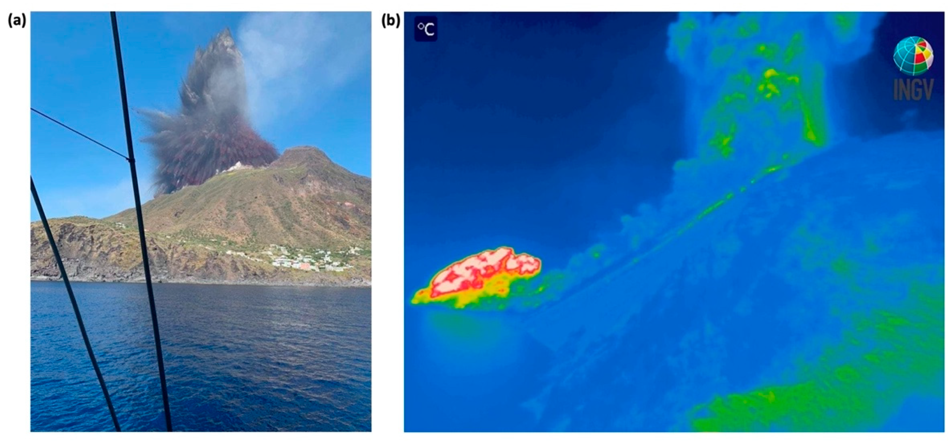
2.1. Thermal Observations from Fixed Camera and Satellite

Data acquired by the Flir A320 Thermal Camera installed at the INGV-OE Monitoring Station SPT (Stromboli Pizzo Thermal) located at Pizzo sopra La Fossa, 918 m above sea level (ASL), were processed. We considered the hourly frequency of the explosion and the dispersions of the material involved as follows (see Appendix A for details):
C D = F h · D h
where F h is the hourly frequency of the explosions and D h is the dispersion (calculated as number of pixels of the thermal anomaly) and CD is defined as the cumulative dispersion.
The choice is justified by the observation during the long-time intervals of ordinary explosions: average or low-energy events make F h and D h entirely uncorrelated, while during bigger ordinary events, the system responds by lowering the frequency to maintain its balance.
Accordingly, we plotted the CD for the period 3 April 2019 to 3 July 2019 (when the camera was destroyed by the paroxysm) related to each area filtered by a simple 49-sample mean average (Figure 3a). Another interesting result obtained from the automatic detection of explosions from videos is the attribution to the different crater area of every single explosion. If we plot both the Cd related to each area of emission (north and south), the results can be summarized as in Figure 3b.
We processed multi-spectral data acquired by MODIS and SEVIRI satellite sensors by using the HOTSAT thermal monitoring system [8,9]. This system allows for the automatic detection of thermally anomalous pixels (hotspot) and quantifies the thermal activity by computing the radiant heat flux. During the first six months of 2019, we find hotspots mainly in MODIS images, since they are more sensitive to lower thermal energy (see Figure A2a, Appendix A), but after 3 July we followed the more energetic phases of the eruption thanks to SEVIRI (see Figure A2b and Figure A3, Appendix A). Figure 3a shows good agreement between the MODIS-derived radiant heat flux during April–3 July 2019 and the cumulative dispersion computed from the ground-based thermal camera. Indeed, the higher values registered by MODIS from June measure the continuous spattering activity, which provides a persistent thermal anomaly in the vent area. The MODIS signals are thus a consequence of the increasing explosive activity that is assessed by the cumulative dispersion.

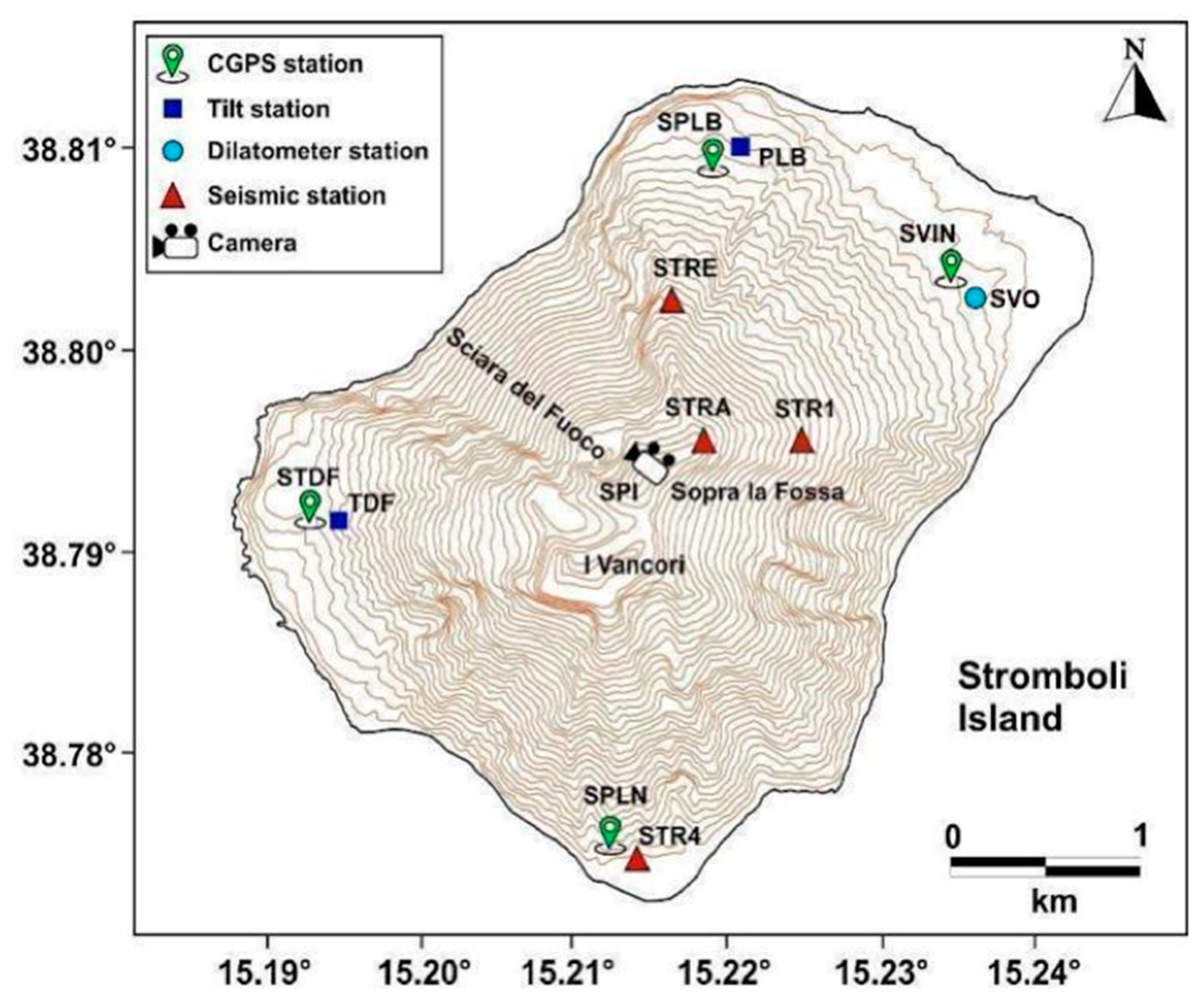
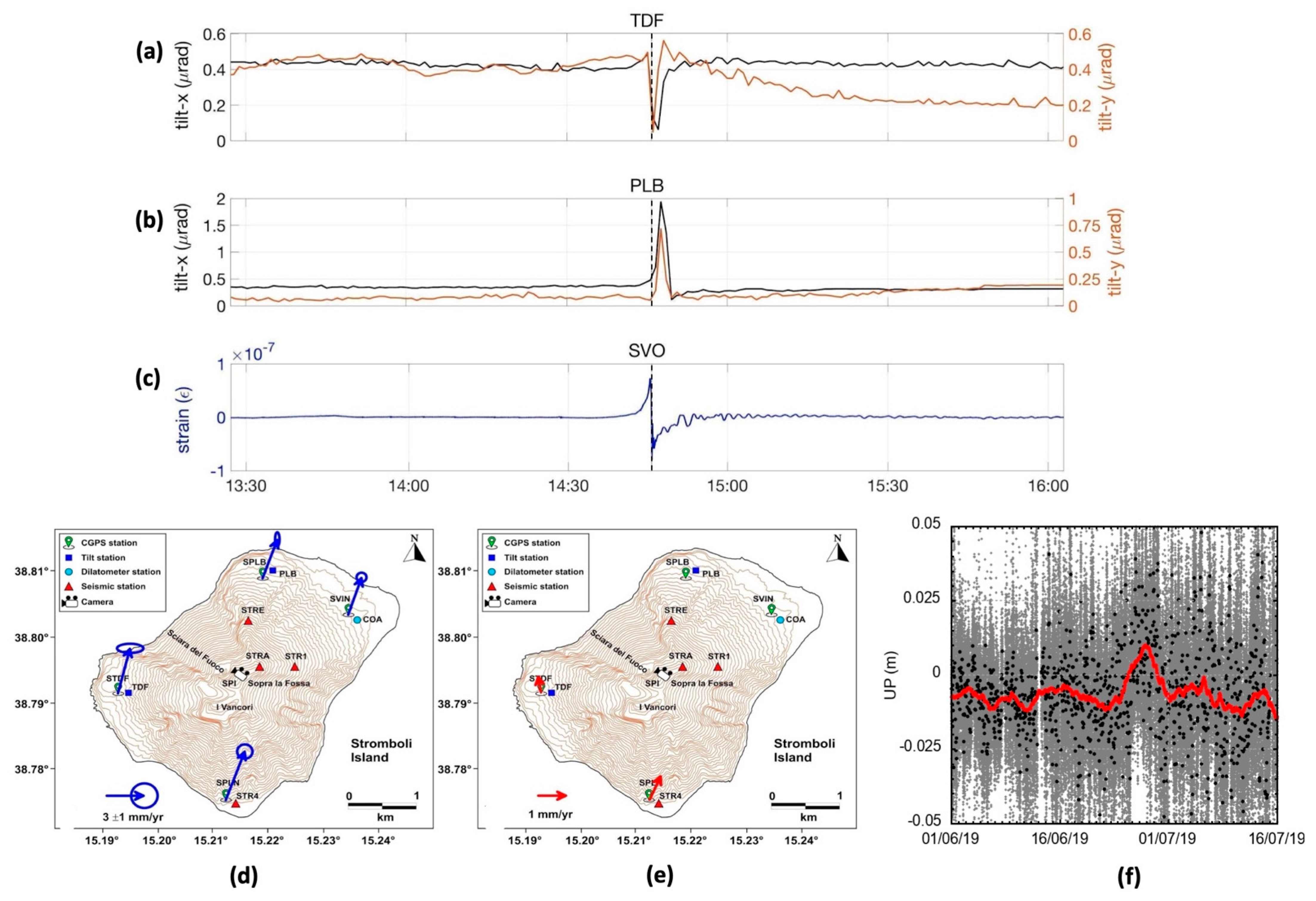
2.2. Ground Deformation and Seismic Data

Long-term tilt signals (see Appendix A for details) did not show any variation until the end of May when the N275°E component of TDF began a lowering trend (tilt down toward summit area). No evident changes were recorded in the other TDF component or in PLB signals (Figure A4Appendix A).
Tiltmeters recorded changes before the 3 July 2019 paroxysmic explosion, indicating an uplift of the summit area (Figure 4a,b). Variations are small (about 0.1 microrads) and detected about 2–3 min before with PLB and 3–4 min with TDF. During the two explosive episodes of July and August 2019, tilt showed variations of 1–2 microrads.
No meaningful changes in trend or abrupt variations are evident in the daily time series of global navigation satellite system (GNSS) data (Figure A7, Appendix A), excluding any possibility of deep or shallow intrusion of large dimensions preceding the two paroxysms of July–August 2019. We estimate velocities, uncertainties and noise properties of the four GNSS stations using HECTOR software [10]. A clear difference in terms of velocities is shown by the southern sector of the island (Figure 4d), and this feature is clearer if a “SVIN-fixed” reference system is applied (Figure 4e). The residual velocities of STDF and SPLN station show a contraction between the northern and southern sectors of the island (Figure 4e).
The high rate (1 Hz) GNSS data show large displacements related to the 3 July 2019 paroxysm (Figure A8a, Appendix A). However, they are of unclear origin and possibly due to the large dispersion of ash and hot water vapor during the event that influenced the propagation of the GNSS signal. The 30 s-GNSS data recorded at SPLN station in June 2019 show a clear uplift between days 23 and 28 (Figure 4f), indicating a possible shallow propagation of volcanic fluids very close to the southern edge of the island just a few days before the 3 July explosion. This variation, although of limited magnitude, is an anomaly in the high frequency time series of the SPLN station. Moreover, SPLN is the only GNSS station that recorded a variation in this period, probably due to its position very close to sea level and in the southern sector of the volcano.
Before the 3 July paroxysm, the SVO strainmeter recorded intriguing signals (Figure 4c): comparing the precursory effusive phase recorded by the monitoring camera installed near the southern vents of the main crater, the minimum strain value (frame 14:34:32) occurs about 11 min before the paroxysmal explosion (frame 14:45:40) [5].
The two paroxysms that occurred in 2019 have a similar strain time history: Di Lieto et al. [6] show the details of the strain recorded a few minutes before both events and evidence a correlation among them and the paroxysm that occurred in 2007, suggesting a common source mechanism. During the months preceding the July paroxysm, no significant changes in the unfiltered strain data were observed.
Fast rising within the conduit of gas bubbles generates seismic signals in the shallow part of the feeding system [11] in the frequency band 2–50 s, which are also visible on tiltmeters and strainmeter data, as a transient of about 50–200 nrad [12] and 2–4 nε, respectively. Hence, we focused on the VLP frequency band. We will refer to strain transients recorded in this band as “strain VLP”. From a statistical analysis conducted on almost 100,000 strain VLPs recorded in the period June 2018–December 2019 by the SVO strainmeter, we found that all the examined strain VLP parameters routinely analysed by the scientific community on seismic signals change slightly about 30 days before the 3 July event, showing a weak correlation once they are plotted together (Figure 5b–f). Indeed, clearer variations occur in strain VLP shape, which abruptly changes on 3 June and then again on 25 June (Figure 5a). The significant number of strain VLPs belong to two different families (Figure 6a): the first family contains events characterized by a pronounced quasi-symmetric positive, dominant, bell-shaped peak with an oscillation before and after the main peak, clearly visible from 3 June, in contrast to the second family, whose predominant characteristic is a longer oscillation without a prevailing peak, which appears from 25 June as the first one suddenly disappears. The first family consists of a dilatational strain transient with durations of 30 s, while in the second family dilatational and compressional phases are more balanced, suggesting a variation in the visco-elastic medium characteristics, with the same values for their amplitude and duration.
The 28 August paroxysm was not preceded by changes in any parameter of the strain VLPs. It occurred during an active phase, with all the monitored parameters already modified with respect to the normal activity and with a very high amplitude of the volcanic tremor [5].

2.3. Seismic and Strain Data Comparison

In Giudicepietro et al. [5], seismic data (with a focus on volcanic tremor, explosion quakes, volcano–tectonic and VLP events) from November 2018 to September 2019 are analysed, showing the presence of significant variations through the whole month preceding the paroxysm of 3 July. Introducing a new parameter called “VLP size”, differences in VLP shape recorded by the seismic network were observed by Giudicepietro et al. [5], who linked temporal evolution of explosive source to a higher gas content in the Strombolian explosive activity, and also by Chouet et al. [11], who found a correlation with activity at the different vents.
In line with Giudicepietro et al. [5], we performed a cross-correlation analysis of a selected dataset of VLP recorded by the seismometer installed at STRA station (hereinafter “seismic VLP”), which is located 500 m away from the vents at about 850 m ASL, to verify the changes in strain VLP shape. Based on strain VLP event arrivals, seismic waveforms were triggered and extracted from the vertical component of seismic recordings in the time interval 1 June–3 July 2019. We collected about 2400 seismic VLPs filtered in the frequency band 2.5–20 s. With the aim of investigating similarity and waveform variation over time, seismic traces were cross-correlated with each other. Choosing 40-s-long windows and a cross-correlation coefficient threshold of 0.8, seismic traces were grouped into 11 families. Only families consisting of at least 15 events, whose stacked and normalized waveforms are shown in Figure 6b, were selected. The time variation of the daily occurrence rate of events of each of the six families selected has also been carried out (Figure 6c). Results show an increase in the event number starting from 25 June and indicate that family 1 is the most populated one, and seismic VLP events belonging to this family were recorded during the whole period (Figure 6c). The main variation associated with this event type is a decrease in number occurring around 22 June, which was then followed (on 27 June) by an increase until the paroxysm of 3 July. Furthermore, after the family 1 occurrence rate decreases, seismic VLP waveforms were grouped in several families (Figure 6c). After around 22 June, all the different seismic VLP shapes found by cross-correlation were observed. We highlight that seismic VLP types belonging to families 3 and 4 have similar waveforms with respect to the most frequent ones (Figure 6b). After 25 June, beside seismic VLP belonging to family 1, only those of families 2, 5 and 6 are observed (Figure 6c). Visual inspection of waveforms allowed us to identify similarities between the seismic VLP event shape of family 1 (Figure 6b) and the shape of the first kind of strain VLP (Figure 6a) and between the seismic VLP event shape of families 2 and 5 (Figure 6b) and the shape of the second kind of strain VLP (Figure 6a). It should be noted that while in seismic traces seismic VLP events belonging to family 1 have been pinpointed throughout the period, strain VLP events of kind 1 disappear after 25 June. The slight differences between seismic families contrast with the clear strain VLPs’ shape changes. Therefore, we focused on seismic VLP events belonging to family 1, split the time interval into two periods, 1–24 June and 25 June–3 July, and computed stacks. Stacked and normalized waveforms of the two periods, reported in Figure 6d, highlight a slight modification of seismic VLP: in the second period, seismic VLP event-stacking is characterized by a longer tail, suggesting decreased damping of seismic VLP events, whereas the frequency tends to remain constant.
The comparison between results obtained by investigating strain VLPs with seismic VLPs confirms a change in VLP shape, and as a consequence in the source mechanism and/or in the fluid properties after 25 June. In addition, seismic VLP component analyses evidenced that this process started a few days earlier and was probably complex, indeed, starting from 22 June and lasting until 25 June, seismic VLP event types belonging to families 3 and 4, which exhibit waveforms similar to those of the seismic VLP of family 1 (Figure 6b–d), were also recognized.

3. Modelling the Volcanic Source

We performed an analytical inversion of tilt, strain and displacement data variations recorded during the five minutes before the explosion (see Appendix A.4. for more details). We used a pressurizing source embedded in a homogeneous half-space described as a simple spherical source [13]. In particular, all available data have been inverted simultaneously using the software developed by Cannavò [14]. The effects of the topography were taken into account by using the method of Williams and Wadge [15]. We obtained a pressure source located under the craters area at about one hundred meters above sea level (Figure 7). The source is characterized by a volumetric expansion of about 10,500 m3. This value found for the source of the explosion is much lower than that evidenced by Di Lieto et al. [6]. This is due to the fact that the model presented in the current manuscript takes into account all available ground deformation signal changes occurring in the five minutes prior the paroxysmal event to estimate the small volume responsible for triggering the explosion. Instead, Di Lieto et al. [6] consider the strain signal variation recorded during the phenomenological phase of the paroxysmal activity that involves both the middle (about 1.5 km b.s.l) and shallower storages. The volume of the pressure source (about 106 m3) is calculated by considering the peak to peak strain variation over the entire signal duration. The different modelling approach used in Di Lieto et al. [6] also conditions the source depth estimate, which has been found to be consequently lower in the present work. Moreover, it is noteworthy that the Mogi’s model [13] does not provide a correct solution for the pressure source located above the elevation of recording stations and, therefore, we limited the maximum values that the “Z” coordinate can assume to the minimum elevation of our stations (about +80 m above sea level). Our solution achieves this value. Despite this limitation, our approach data fit is good (Figure 7). In fact, we obtained a reduced chi-squared χ2 equal to ~1.0 considering an a posteriori standard deviation of 0.01 m and 0.02 m for the horizontal and vertical displacements, an uncertainty of 1.0 μrad for the tilt data and of 0.02 με for the strain data. Seeking to overcome the intrinsic limitation of the Mogi [13] approach, if we exclusively invert the tilt variations deduced by the three summit seismic stations (STRA, STRE, STR1, Figure 2), we obtain a pressure source that is not well-constrained located at an altitude of (+480 ± 620) m with respect to sea level. Therefore, the good result obtained using all available data leads us to believe that the real pressure source representing the five minutes preceding the eruptive explosion is probably not much above the obtained level of +80 m. The estimated small volume variation does not affect the signals recorded at the high-frequency GNSS network. Conversely, it was visible to the borehole instruments due to their high sensitivity. Moreover, it is well known that geodesy alone cannot constrain important parameters such as chamber volume or pressure and that deformation studies resolve exclusively for a volume variation [16] that cannot be compared to the erupted volume. However, the small value that we obtained for the volume variation preceding the paroxysm could suggest a key role played by the continuum gas phase with respect to a supply of new magma, as explained in the following paragraphs.

4. Discussion

The intermittency of Strombolian explosions has been interpreted by Jaupart and Vergniolle [17,18] as a consequence of the periodic collapses of a foam layer formed by the accumulation of bubbles that remain trapped below the magma surface. According to this view, the maximum packing condition is reached when the contact area between bubbles becomes equal to the cross-sectional area of the bubble. Similarly, Chouet et al. [11] proposed a source mechanism on the basis of seismic broadband data and the observed intermittency of explosive eruptions, which point to a degassing process in which gas bubbles rising in the inclined liquid-filled dike tend to concentrate against the upper wall of the dike, thus enhancing the collisions between bubbles and their coalescence. As demonstrated in laboratory experiments with analogue fluids [19], localized bubble concentration against inclined surfaces makes slug flow unavoidable at all but the lowest gas-flow rates for non-vertical conduits. Therefore, a crucial element in this degassing process is the inclination and the shape of the conduit.
Recently, Oppenheimer et al. [20] have proposed, on the basis of analogue laboratory models, the important role of near-surface (down to 800 m) crystallization and the variations of the crystallinity and the interactions of crystal-bubbles in regulating the intensity of degassing and explosive activity. These authors proposed a “weak plug” model for Strombolian explosions, evolving from low viscosity style towards more crystalline, a stronger and less permeable plug corresponding to larger events. These last events are characterized by an increase in the crystallinity, determining a different conduit condition and larger size explosions. This model predicts some features of the Strombolian explosions, such as the variability of their sizes, duration, pulsation and fountaining according to the degree of near-surface crystallization, but suffers from a lack of a quantitative explanation of geophysical signals. Moreover, in Caracciolo et al. [21] petrological evidence for a ‘soft plug’ model based on observations of earlier explosions are discussed.
To find an eruptive mechanism that could take into account the large spectrum of geophysical data, the direct observation of the paroxysm and the nature of the erupted material, we decided to adopt the “push and go” model proposed for the feeding system of Mount Etna volcano in Ferlito [22]. The magma is described not as molten rock residing at a certain depth within the volcanic edifice or in the crust, but, on the contrary, as a flux of fluid continuously moving upwards, in which two vertically distributed portions can be recognised. Below is a solution made of ~70% in volume by a continuum gas phase (mostly H2O) in a supercritical state (density 360 kg/m3) and 30% in volume by basaltic components dissolved in it, named water melt solution (WMS); the overall density is low (1140 kg/m3). At the top of the WMS, the continuous loss of gas, characterising all persistently active volcanoes, will leave a highly dense (2800 kg/m3) basaltic melt, defined as a continuous melt phase (CMP). The CMP has a low enough viscosity to permit the continuous passage of the gas bubbles coming from the degassing of the WMS (Figure 10a). The transition between the WMS and the CMP can be erratic within the plumbing system. In this new paradigm of magma, the eruptions can be considered to occur due to a significant pressure increase within the WMS in the deep plumbing system, which cannot be kept confined by the weight of the overlying basaltic melt (CMP). This process can be viewed like a piston acting within a cylinder, in which the overpressure and expansion of the gas-rich WMS appears crucial, able to push the high-density basalt of the CMP up to the surface effusion. There are two main causes for the overpressure within the WMS: an increase in the gas flux from a deeper source or a decrease in the permeability of the CMP, which in turn could be caused by a viscosity increase in the CMP due to the cooling of the melt and incipient crystallization (see [20]). The eruption will be effusive, with lava flows, if the CMP is able to dynamically contain the expansion of the WMS below; whereas, if the CMP is unable to confine the WMS expansion, the latter will be violently emitted and the resulting eruption will be an explosive paroxysm.
From a joint comparison among all data, we identified two different volcanic state phases: a precursory phase, starting in early June 2019 (yellow and blue filled rectangles in Figure 8) that consists of a medium and a short pre-paroxysmal time, and a paroxysmal phase, starting on 3 July (red filled rectangle in Figure 8), that includes all the eruptive volcanic activity, characterized by effusive activity and by a second paroxysm on 28 August.

4.1. The Precursory Phase

From June 2018 to the end of April 2019, we do not observe any significant variation in the measured parameters. At the beginning of June there is a significant increase in the cumulative dispersion parameter (considering the medium value of the preceding months), which is directly connected to the energy of the explosive events, and of the number of strain VLPs, whereas GNSS does not show any variation. MODIS data revealed almost continuous thermal anomalies from June 6, showing a radiant heat flux curve with an increasing trend reaching a maximum value of 0.45 GW on 2 July at 12:00 GMT. Tilt evidences a trend change on the TDF N275°E component, which, however, has no counterpart on the other components or the PLB data (Figure 8), suggesting a local source for this variation. Such a lack of “depth” related signals indicate that this phase of unrest must be associated with the uppermost portion of the feeding system, specifically the CMP. Considering that the cumulative dispersion parameter indicates an increase in the magnitude, not in the number, of the explosive events that are caused by the breaking of gas bubbles at the surface of the CMP, it must be deduced that more energetic explosions must be generated by larger bubbles or by bubbles that have a higher gas overpressure. The large rose-shaped incandescent ejecta observed during this phase (Figure 1) would suggest the first hypothesis is more plausible, and large gas bubbles are more likely. Since the most efficient mechanism to form bubbles within a basaltic melt is coalescence, it must be inferred that the viscosity of the melt had to be sufficiently low to allow congruous bubbles mobility (Figure 10a). It can also be deduced that the flux of hot gases passing through the CMP was high enough to maintain a thermal state able to compensate the heat dispersal and therefore hinder crystal nucleation and growth, thus retarding an increase in the CMP viscosity (see Ferlito [22], p. 19). In this first phase, we can reasonably say that the gas flux and therefore the WMS flux in the Strombolian feeding system was high; unfortunately, the lack of a gas sensor network, such as the one set up at Mount Etna, which has allowed us to explain the contribution of the gas flux to the 28 December 2014 eruption (Ferlito et al. [23]), prevents us from making a similar quantification for Stromboli. Indirect confirmation is reported by Inguaggiato et al. [24,25], who found an increase in CO2 soil emissions starting from June, weeks before the paroxysmal event. These data also show higher variance with respect to previous recordings, which index the instability of the volcanic activity.
A similar indication is provided by the increased number of strain VLPs belonging to two main families (Figure 8 and Figure 9). It should be noted that in the first phase, until the first days of June, the feeding system was in an ordinary state and the boost of the gas flux was somehow accommodated by a corresponding increase in the gas flux from the summit craters without any evident change within the feeding system. This first period was followed by a significant variation in the radial tilt and by a sudden appearance of family 1 strain VLPs, which persists until 25 June when family 2 becomes predominant. Waveform analysis of seismic VLP events confirmed the changes occurring in this period (Figure 6). Seismic VLPs at Stromboli are interpreted as being due to pressure change caused by the generation or the ascent of a gas slug in the volcanic conduit [11,26]. Their waveform similarity has been studied in the literature in order to investigate their characteristics in terms of steady activity and changes related to eruptive activity [27,28,29]. After 25 June, several families exhibiting different waveforms appeared (Figure 9) and waveforms belonging to family 1, recognized throughout the period (1 June–3 July), underwent modification in oscillation duration (Figure 6b), suggesting changes in the source mechanism or in the damping property of the medium.
As is known from simplified models of seismo-volcanic sources [30,31,32], the resonance frequency and damping of the system is strongly influenced by the nature of liquid and gas content. Moreover, since seismic VLPs are linked to inertial displacement of material in which they propagate [33,34], the different characteristic waveform of two types suggests two origins: a variation in mechanical magma properties or a different location. In Giudicepietro et al. [5], all seismic VLPs show little variation in incidence angle and azimuth and, starting from 25 June, become very localized. The locations do not show remarkable variations before or during the eruptive phase of summer 2019. These observations seem to reinforce the first hypothesis. In contrast, an explanation of strain VLP shape characteristic is not available in the literature: this work is a starting point in understanding the volcanic processes on which these observations are based.
The variation of these parameters indicates that during this phase, starting on 25 June, the volcanic edifice was reacting to an overpressure of the WMS that the system was unable to discharge through the CMP and the summit craters (Figure 10b). A question that needs to be addressed is whether this different behaviour can be related to a decreased permeability of the system or to an increase in the WMS flux. There is no easy answer, but the products emitted during the short paroxysm of 3 July, in spite of a similar chemical composition, had two distinct textures: the partly crystallized “brown” (Figures S1 and S2) and the totally glassy “blonde” (Figures S3 and S4). The crystal content of the brown indicates that before the paroxysm the CMP must have reached a considerable degree of viscosity, which in turn could have decreased the permeability. Moreover, during the increase in the WMS flux, occurring in the first phase, only the gaseous component was emitted and therefore discharged from the feeding system, whereas the basaltic (melt) component was mainly retained within the uppermost portion of the feeding system, increasing the size of the CMP up to the point in which the gas flux was unable to provide the heat sufficient to maintain low viscosity to hinder the crystallization of the CMP. The decreased CMP permeability delayed the flux of the gas bubbles through it and must have therefore led to an overpressure of the WMS. Such an isotropic pressure must have acted against the entire upper portion of the feeding conduit, boosting a deformation that can be considered responsible for the radial tilt variation observed at the TDF station (see Figure 8). Now, any volcano being a complex dynamic system, it appears obvious that such a condition of instability is temporary and must evolve somehow. Unmistakable signs of the dramatic evolution began to show from 25 June, one week before the paroxysm. The number of VLPs increased significantly and so did their intensity. At the same time, the energy of the explosions had a conspicuous boost. The radial tilting (TDF N275°E component) increased notably and the SPLN GPS station showed an uplift (Figure 4f). This further rise of the physical signals was the prelude of the paroxysm and can be interpreted as the last bearable increase in WMS overpressure before the break-up of the CMP.
The 3 July paroxysm that occurred at 14:45:45 UTC was the sudden and violent emission of the CMP unable to contain the dramatic pressure increase within the underlying WMS, which produced an inflation of 10,500 m3 and was preceded, about one minute earlier, by a shallow (800 m deep [5]) volcano tectonic event (VT), suggesting a fracture in the base layer of the CMP column. According to the proposed “push and go” model, the explosion would occur at the very moment at which the overpressure in the WMS overcomes the confining pressure of the CMP above it (Figure 10c). We maintain that our modelled pressure source is roughly located at the interface between the WMS and the CMP. Exclusively for speculative reasoning, we would like to verify how large the CMP would need to be to keep the underlying layer (WMS) confined by its own weight. Considering that the pressure source is located at about 700 m below the surface, a hypothetical cylindric conduit representing the CMP and having a volume equal to the estimated “ΔV”, to roughly balance the pressure of the modelled source, should have a radius of about 2 m. This value is compatible with the dimensions of the open vents usually visible at the summit craters of Stromboli.

4.2. The Paroxysmal Phase

What might be of further interest is examining the 75 min preceding the paroxysm. In Figure A6, from minute −90 to minute −75, the only notable variation is given by the strain VLPs occurring at about a 5 min intervals. From minute −75 to minute −60, the positive strain has an increase that reaches a peak of 0.55 × 10⁻⁸. This positive strain could have been caused by an overpressure likely due to a boost in the WMS flux. In the following 50 min, the excess flux was discharged, passing through the overlying CMP and thus significantly decreasing the positive strain. Two distinct patterns of strain release are notable (Figure A6): at the beginning the rate was fast, in the first 5 min it decreased by 0.2 × 10⁻⁸ with no strain VLPs associated; whereas from minute −55 to minute −10, the strain decreased with a slower rate from 0.2 to −0.25 × 10⁻⁸ and in a discontinuous “step way” fashion, in which the occurrence of each strain VLP event is associated with an immediate step of strain decrease. This information suggests that the strain VLPs generate at the interface between the WMS and the CMP are probably associated with the transition of WMS from a continuous gas + melt flux to a discrete flux of gas (bubbles) within the melt. Two such patterns of pressure release can be interpreted as the contemporaneous existence of two distinct depressurization modes: a “continuous” mode, in which the pressure decrease is due to lava emission through the summit vent and/or gas discharge through the articulated network of fractures that opens at the summit of Stromboli; and a “discontinuous” mode, in which the pressure in the WMS is released through the sudden passage of the gas through the interface with the CMP.
Finally, the last 10 min before the paroxysm are particularly interesting: the strain increased one order of magnitude in less than 10 min; such a sudden and fast increase is not easily explainable as the result of an augmented viscosity of the CMP. What can be hypothesized instead is a dramatic increment in the WMS flux, which was too fast to be released through the CMP. In fact, the travelling time for the gas bubbles to pass through the CMP is in the order of a few minutes, but if the flux increase is faster the system cannot release the gas overpressure in the WMS. The lack of strain VLPs just before the paroxysm is therefore indicative that the gas of the WMS was not able to pass through the CMP, but instead pushed its entire mass (the brown) upwards that was entirely erupted in a few seconds along with the WMS that constituted the glassy texture (the blonde).
The violent emission of the CMP and the WMS occurring on 3 July has strongly modified the uppermost portion of the feeding system. A consideration needs to be made: the very fact that after the sudden emission of CMP and WMS there was no collapse of the summit edifice indicates that the material that was expelled was immediately reintegrated by the rise of deeper melt. Indeed, the eruption continued after the paroxysm with the emission of a lava flow and a regular explosive activity from the summit craters, indicating that the conduit was filled up again with the CMP. A final consideration needs to be made on the paroxysm that occurred on 28 August (Figure A6): the strain curve in the 90 min preceding this second paroxysm appears to be slightly similar to the one of 3 July, but is much smoother and more importantly there is a lack of significant strain VLPs.

5. Conclusions

The paroxysm of 3 July 2019 prompts a general reflection: although an impressive number of monitoring devices have been installed for many years on the island, such a paroxysm occurred without any meaningful variation of the geophysical parameters used for the evaluation of the activity of the volcano (see, e.g., [4,5,7,24]). Volcanic tremor, number of VLP events, ground deformations and earthquakes all showed small unclear variations: we have attempted here a careful revision of “hidden” characteristics of these signals to propose a set of parameters able to detect a change in the state of the volcano, which might lead to unrest or even a paroxysm, so as to help prevent dangerous consequences. However, the parameters considered during the monitoring of the activities of Stromboli volcano is not the only aim of our research: indeed, a step beyond needs to be taken in order to understand why the monitoring of major or paroxysmal events at Stromboli volcano is so elusive and sometimes difficult to interpret. Small variations observed in the geophysical signals recorded in Stromboli could be related to two factors: the small quantities of volcanic fluids involved in Stromboli and the role of gas in their evolution. Hence, we apply a conceptual model previously proposed for Mount Etna volcano (the so called “push and go”) that fits the observed variations occurring at medium and short term before the paroxysm. In our opinion, a high rate of (N > 100/day) and predominance of family 2 strain VLPs over family 1 strain events indicates a high likelihood for an explosive event within the next week to 10 days. In this sense, this information could improve our capability to forecast dramatic events such as the one that occurred in July 2019. Regarding the model, we are aware that, from now on, a more detailed investigation must be carried out at Stromboli and at other basaltic volcanoes to verify its limits, its possible applications, and to investigate some aspects that are still unclear.
Performed data analyses and integration of proposed parameters, estimable/retrievable from real- or near real-time data, helped us shed light on the processes leading to the 3 July Stromboli paroxysm. The following parameters and their variation over time, could be helpful to evaluate the volcanic hazard from explosive activity at Stromboli:
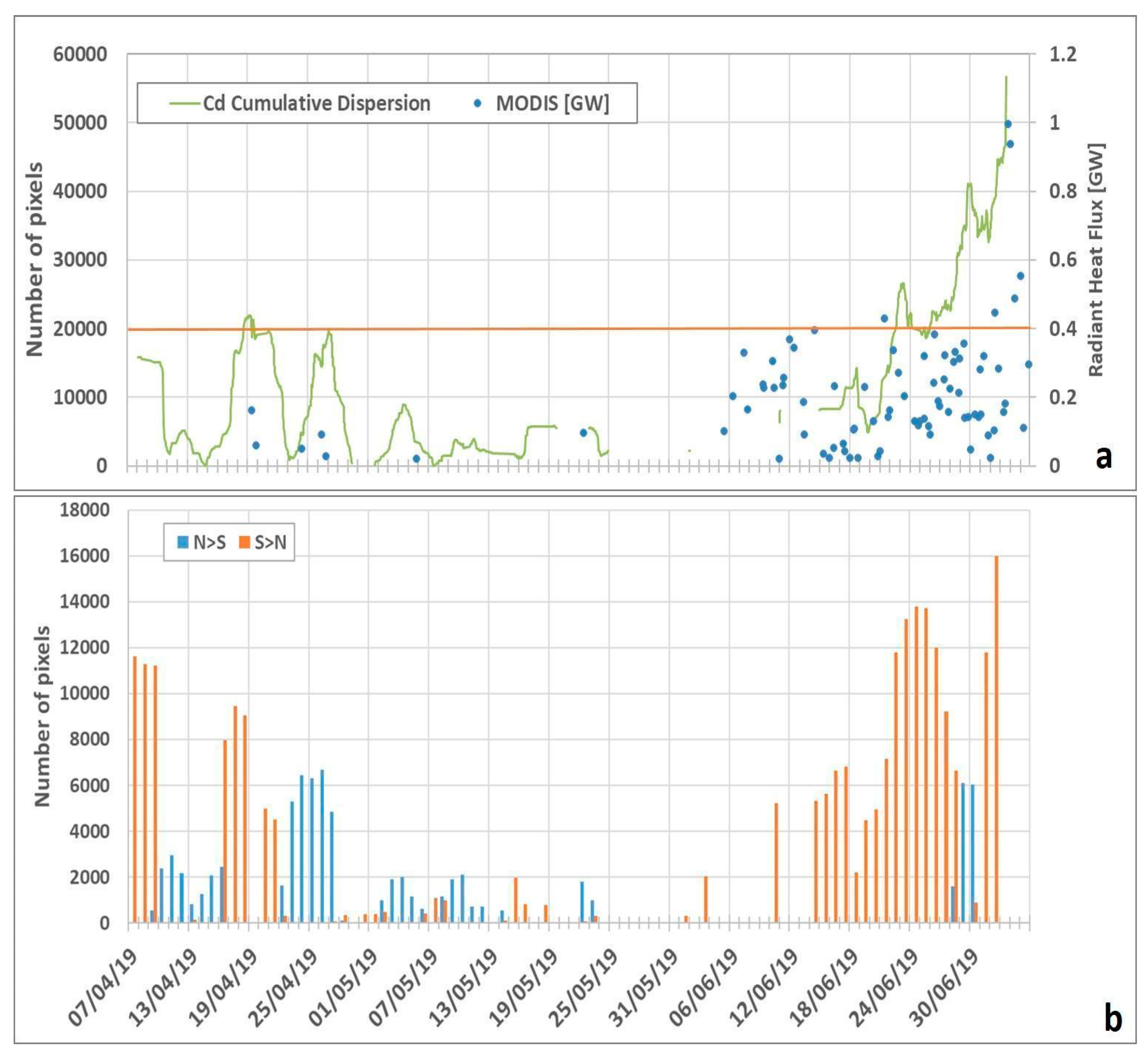
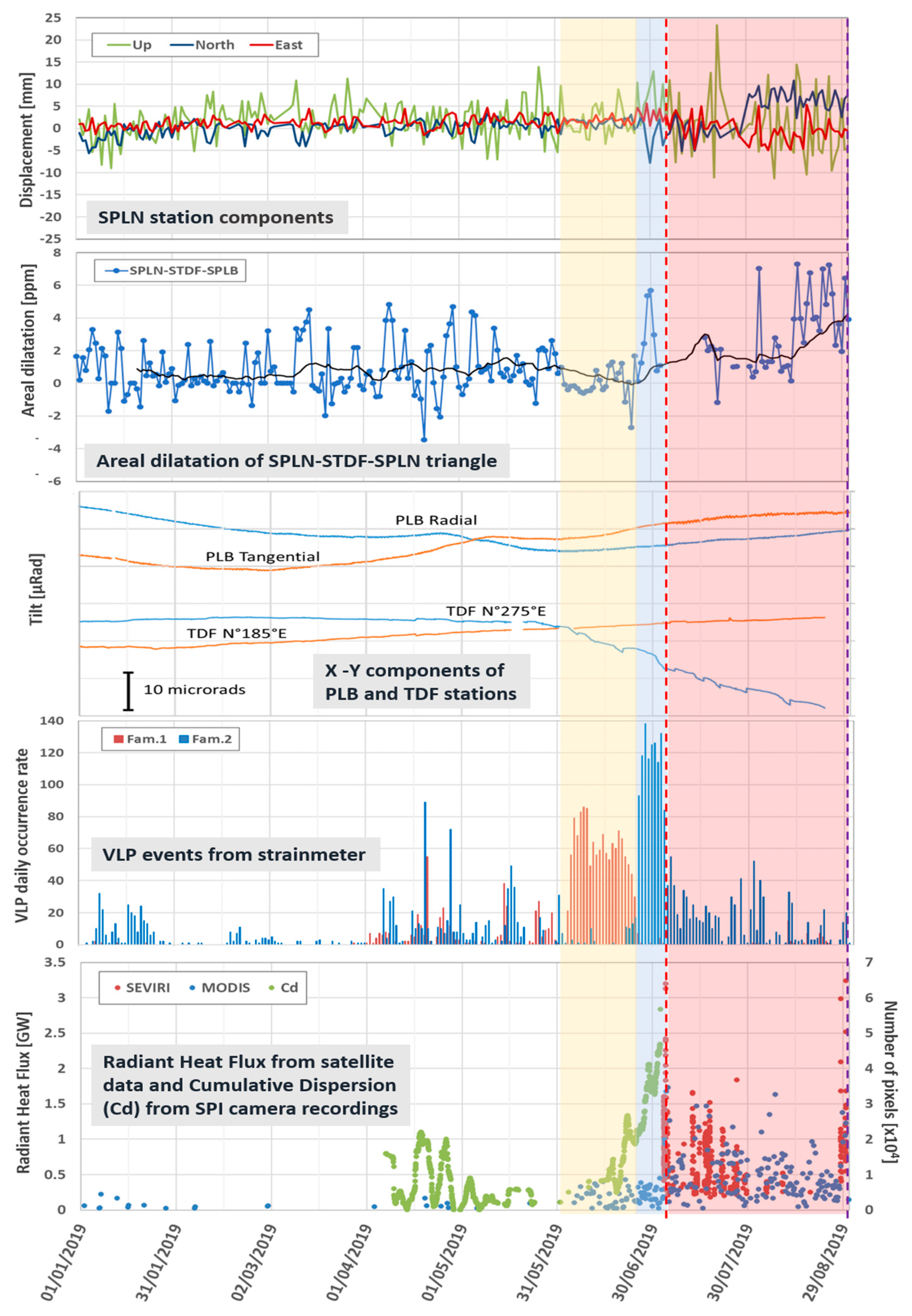
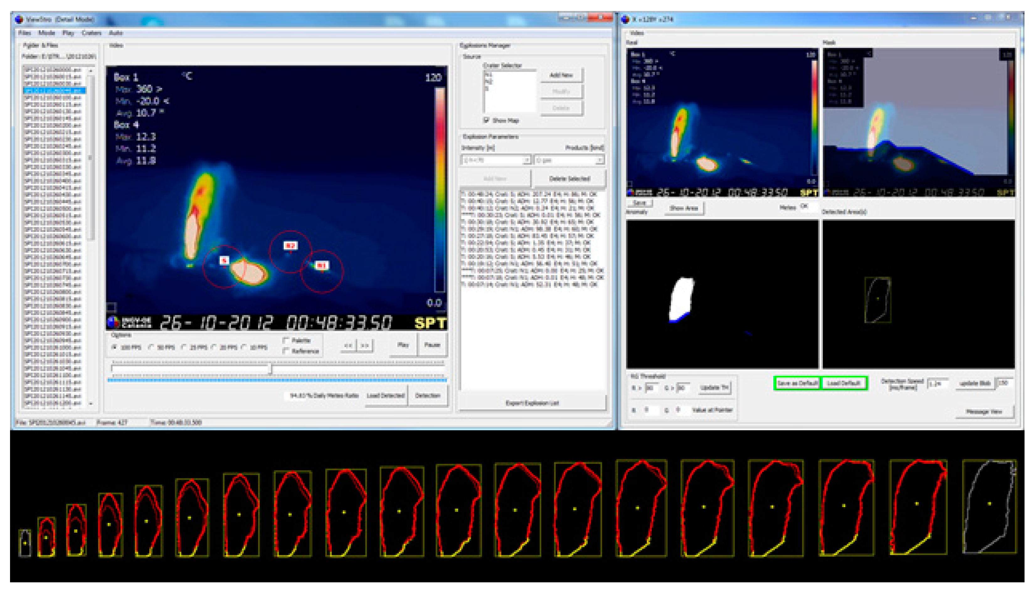
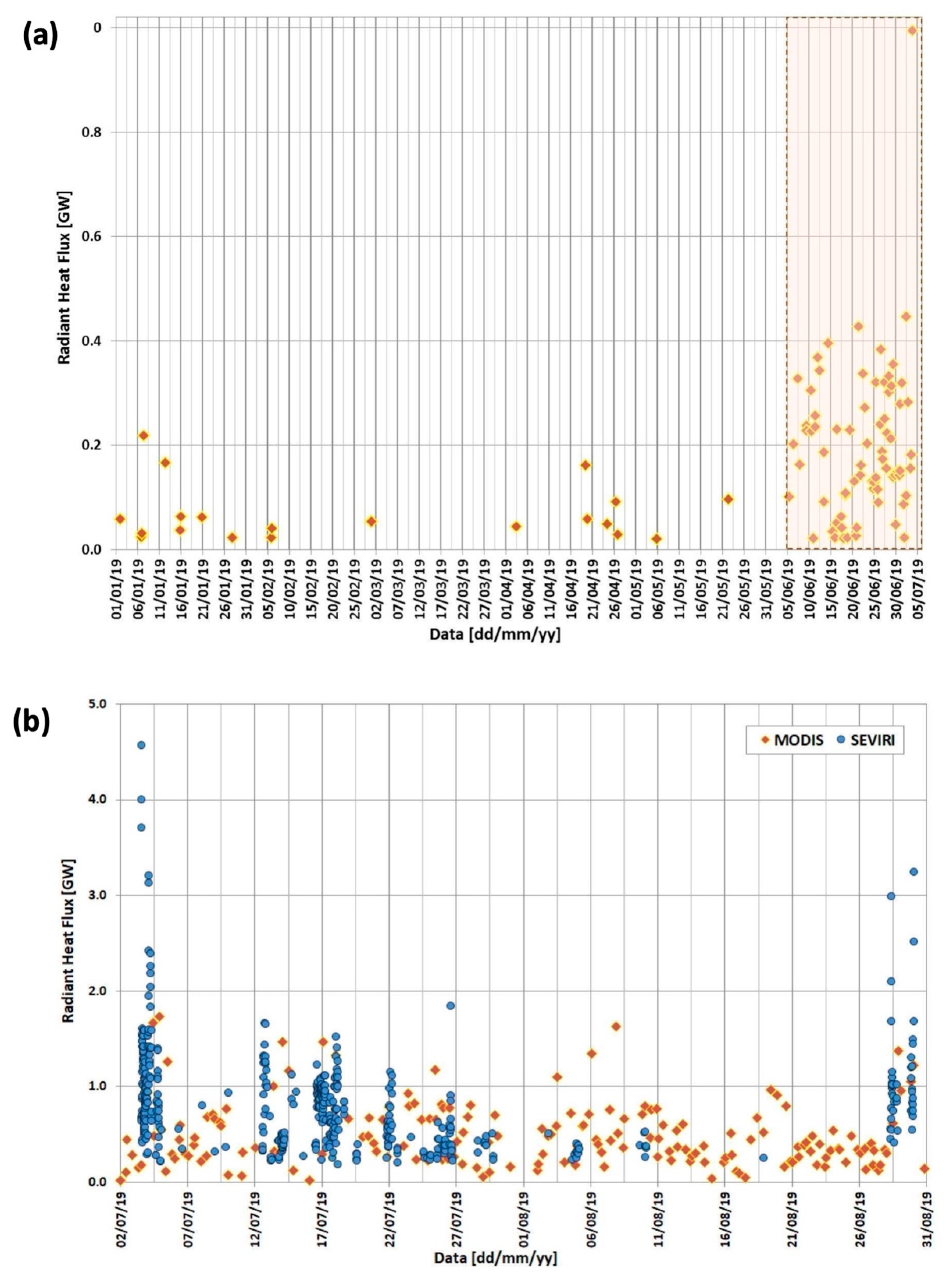
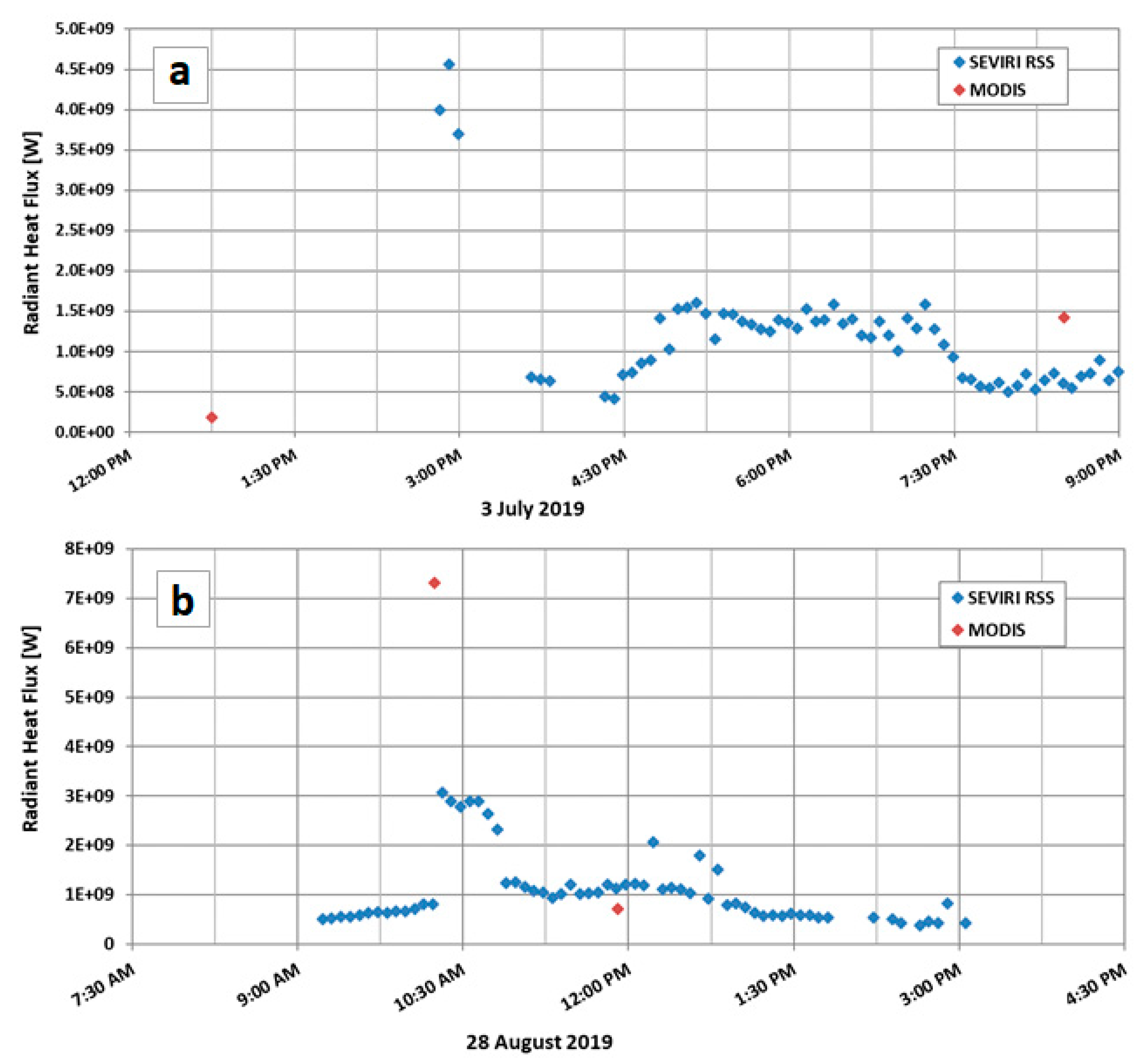
  • Continuous and automatic evaluation of the cumulative dispersion (Figure 8) from video recordings of the summit explosive activity in Stromboli, because the mere observation of the number of explosions occurring from the Stromboli craters is not sufficient and a proxy of the energy involved in the explosive activity is necessary. This value should be coupled with the satellite-derived radiant heat flux to measure the thermal energy due to the extension and persistence of both the vent area and hot deposits as viewed from space.
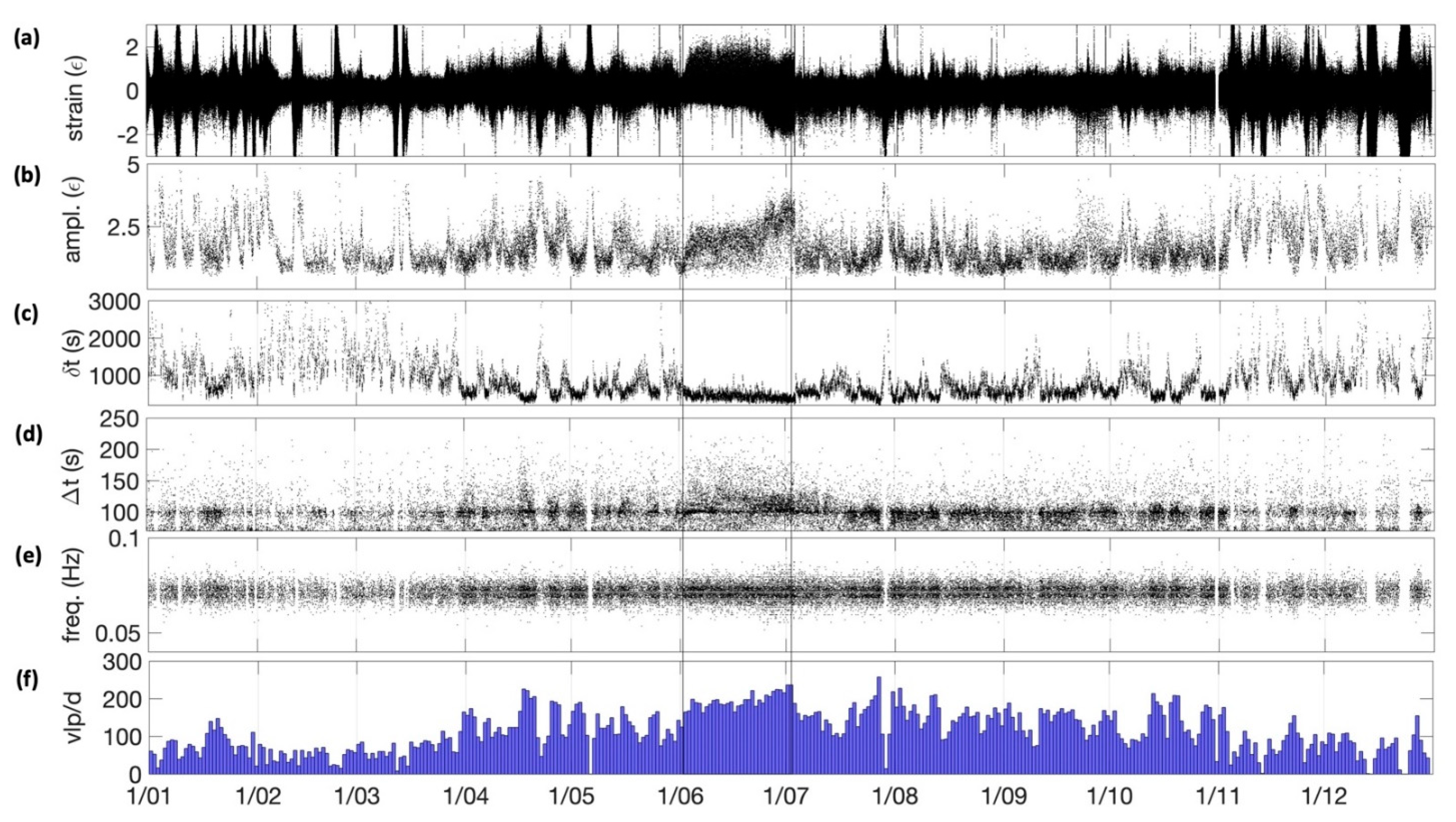
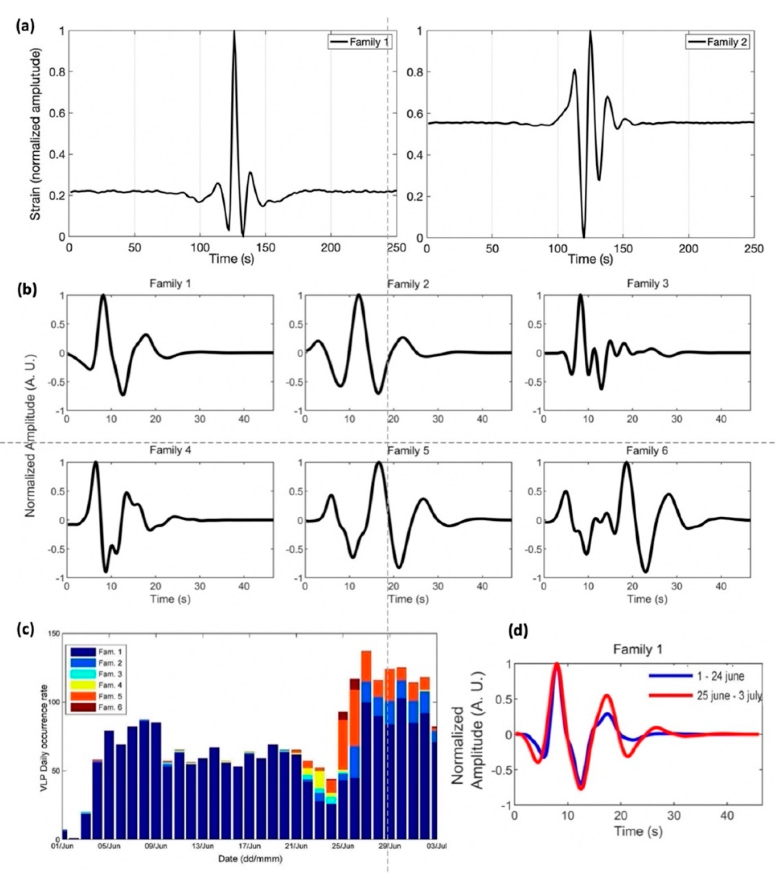
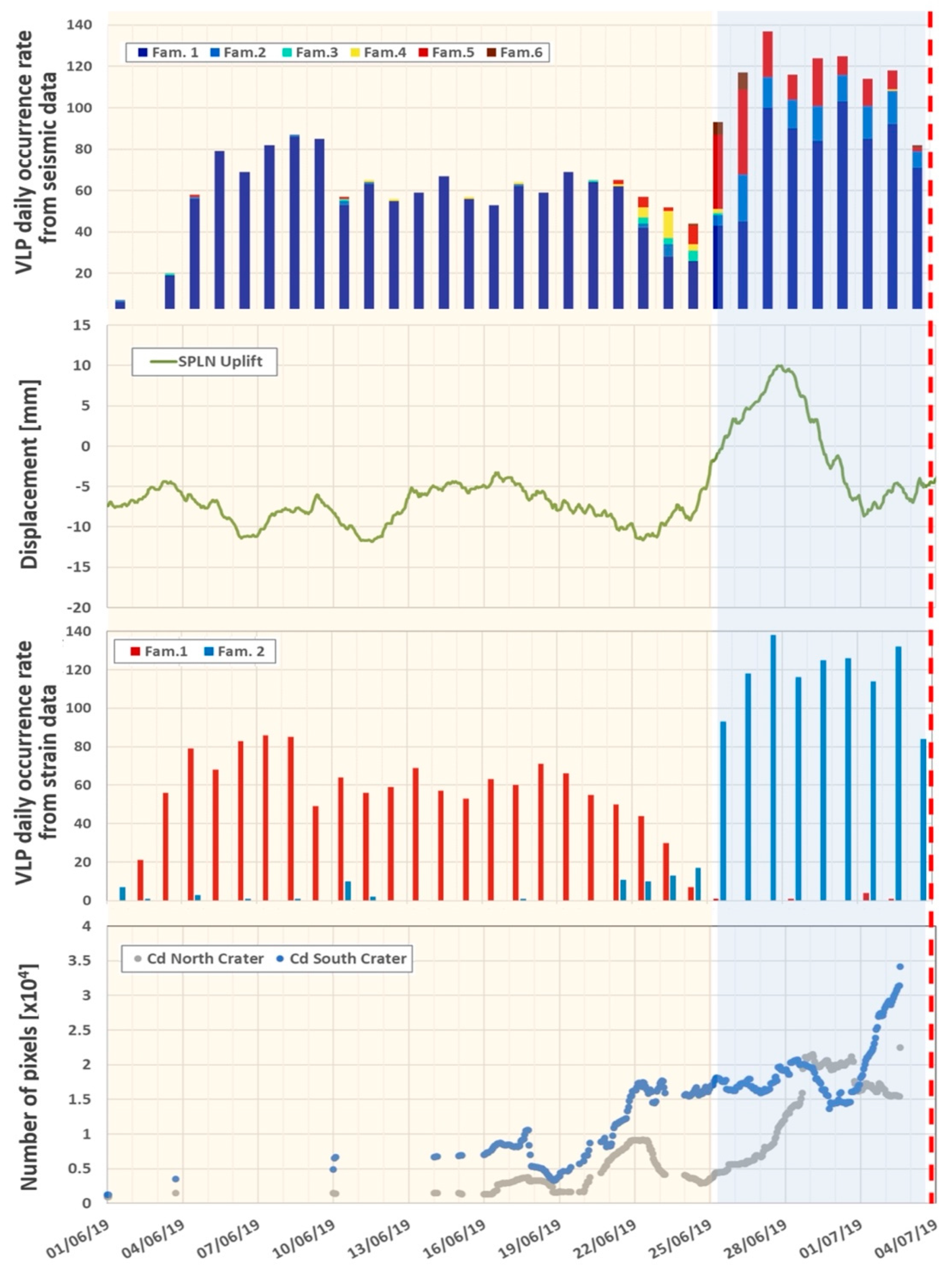
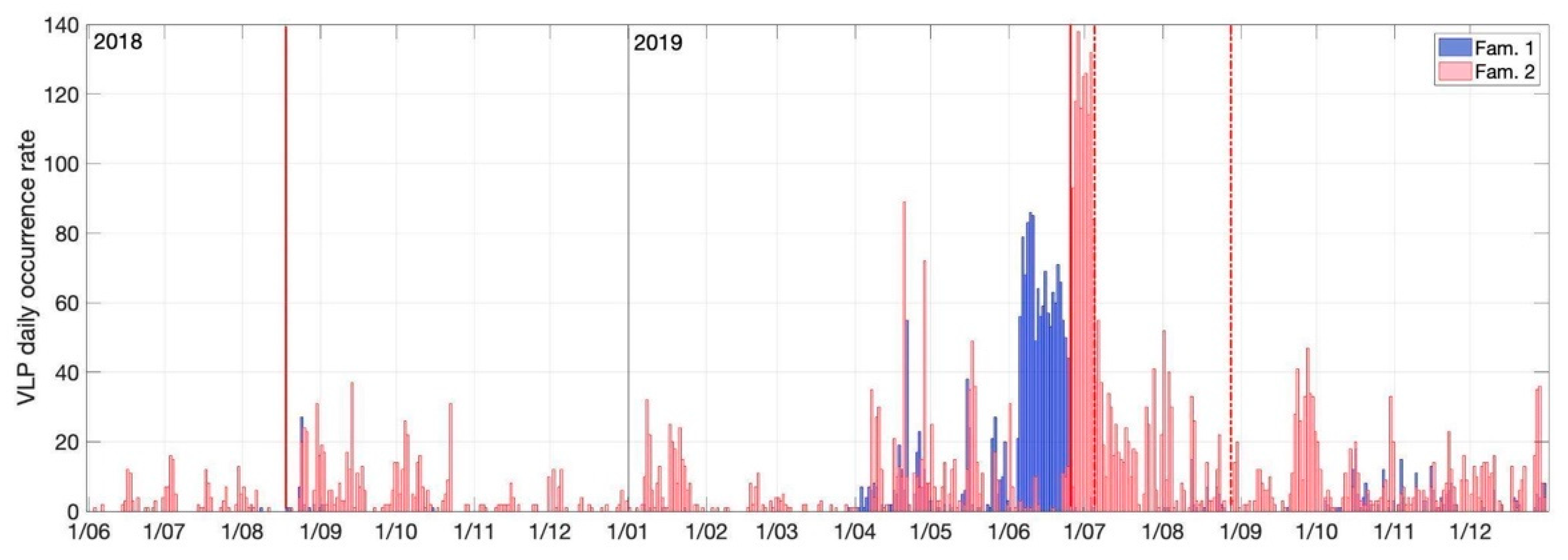
  • Classification of strain and seismic VLP waveforms in different “families”. The transition from one VLP family to another, or the superposition of several seismic VLP families, can be an indicator of changes in the fluid properties, such as the change in permeability of the higher portion of the magma in the main conduit and this can be considered an alteration of the normal condition leading to the mild ordinary explosive activity.
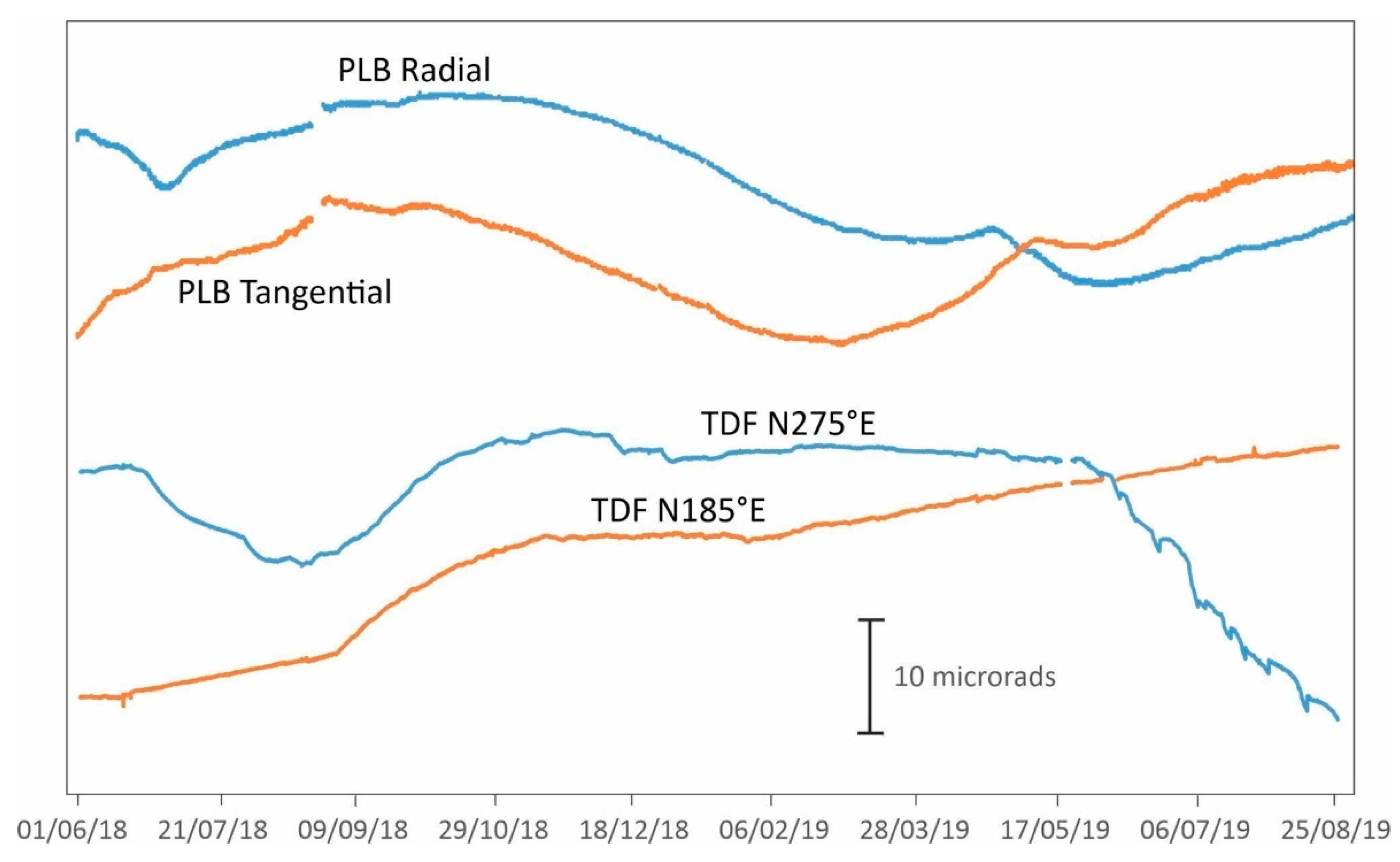
  • Small variations in long/medium term of tilt and GNSS time series, coupled with thermal observations from satellite, must be considered the complementary data whose co-variation can confirm the occurrence of a medium term (one–two weeks) alert of potentially impending large explosive activity.
For these reasons, the present work introduces a new approach to joint multiparametric analysis of monitoring system data. Soon, it could be considered a prototype of an early warning system useful for civil protection purposes on a time scale in the order of weeks/days before a sudden change in dangerous volcanic phenomenology.

Supplementary Materials

The following are available online at https://www.mdpi.com/article/10.3390/rs13204064/s1, Figure S1: Thin section of the “brown” facies characterized by a large number of crystals along with bubbles; Figure S2: Detail of a thin section of the “brown” facies characterized in which the high pyrophoricity of the sample > 35 and the presence of plagioclase as the dominant crystalline phase is visible; Figure S3: Thin section of the “blonde” facies characterized by being largely glassy and extremely rich in bubbles; Figure S4: Detail in thin section of the “blonde” facies in which we can see that the generally glassy texture contains only rare and dispersed crystals.

Author Contributions

Conceptualization, M.M.; methodology, M.M., B.D.L., P.R., P.D.M., S.G. and C.F; satellite remote sensing data analysis, G.G.; thermal camera data analysis, F.C.; tilt data analysis, S.G.; GNSS data analysis, M.M., V.B. and P.D.M.; strain data analysis, B.D.L. and P.R.; seismic data analysis, M.S., P.R. and B.D.L.; volcano source modeling, M.A.; conceptual model, C.F.; investigation, B.D.L., G.G., V.B., F.C., P.D.M., S.G., M.A., M.S. and R.S.; data curation, M.M., B.D.L., P.R., S.G. and M.S.; writing—original draft preparation, M.M. and B.D.L.; writing—review and editing, M.M., B.D.L. and C.F.; All authors have read and agreed to the published version of the manuscript.

Funding

This research was funded by the Project FIRST-ForecastIng eRuptive activity at Stromboli volcano: timing, eruptive style, size, intensity, and duration, INGV-Progetto Strategico Dipartimento Vulcani 2019, (Delibera n. 144/2020; Scientific Responsibility: S.C.). The research has moreover benefited from funding provided by the agreement between Istituto Nazionale di Geofisica e Vulcanologia (INGV) and the Italian Presidenza del Consiglio dei Ministri, Dipartimento della Protezione Civile (DPC—Presidency of the Council of Ministers—Italian Civil Protection Department). This paper does not necessarily represent DPC official opinion and Policies.

Data Availability Statement

The data reported in this paper can be freely downloaded from the FIGSHARE folder https://dx.doi.org/10.6084/m9.figshare.6025748, accessed on 30 September 2021.

Acknowledgments

The authors thank all the technicians and researchers involved in the hard work of maintenance and implementation of the INGV OE and INGV OV monitoring networks. The authors thank Federico Casetta and Pierpaolo Giacomoni for the images of thin sections of “blonde” and “brown” facies. The authors are thankful to the editor and the three anonymous reviewers for their constructive suggestions and comments that allowed us to improve the manuscript.

Conflicts of Interest

The authors declare no conflict of interest.

Appendix A. Details of Data, Methods and Analysis Techniques

Appendix A.1. Quantitative Observation of Camera Recordings

Several software tools have been developed to evaluate the explosive activity observed by the Flir A320 Thermal Camera installed at the INGV-OE Monitoring Station SPT (Stromboli Pizzo Thermal) located at Pizzo sopra La Fossa, 918 m ASL facing the whole summit area of Stromboli volcano. The camera (Figure 2), with a 90° focal length, has a perfect view over the crater terrace, producing a stream that is transferred and stored as RGB (Red Green Blue) videos 320 × 240 at 2fps (Frames per Second) split into AVI (Audio Video Interleave) files every 15 min, resulting in 96 videos per day that are 1800 frames each.
A specific software tool analyses the videos and automatically detects all the explosions from the summit craters, acquiring all the features of the explosive events and estimating a degree of reliability of the detection (affected by weather conditions and integrity of the video files). Every explosion is detected starting from the trigger time up to the maximum expansion of the material ejected traced as a thermal anomaly, as described in Figure A1.
Figure A1. Typical screen of the software tool for the analysis of explosions at Stromboli with the continuous tracing of the maximum extension of every single explosion following its thermal anomaly.
Remotesensing 13 04064 g0a1
The result is a database with the following features:
  • Trigger Time [hh:mm:ss.zzz]
  • Source of emission (vent)
  • Duration of the event [sec]
  • Dispersion, the maximum area involved in a thermal anomaly due to the event [pixel]
  • Height max of the anomaly [m]
  • Width max of the anomaly [m]
  • Frame at maximum expansion
A proxy of the energy release related to a single event has been chosen; the energy related to an explosion is roughly the amount of the ejected material traced by a geometrical parameter. While the height and the dispersion correlate well during the ordinary low energy activity, stronger explosions affect the area involved in the thermal anomaly during the event more than the height of the ejected materials. In conclusion, the dispersion parameter can represent the mass of the material ejected during any kind of explosion. Another software tool has also been realized to link all the files of a period, summarising all the features and plotting its temporal evolutions, choosing an hourly time span. In this way, a proxy of the long period energy release can be investigated based on the simple principle that the more material ejected, the more the energy release.

Appendix A.2. Satellite Thermal Data

For about 50 years, satellite remote sensing has been a widely used technique for monitoring volcanic heat emissions often related directly to the eruptive activity at a specific time [35]. The thermal activity observed is usually quantified by temperature, area, radiant heat flux, and, in the case of effusive eruptions, time averaged discharge rate, i.e., an estimation of the effusion rate. The source of the thermal emission might be a fresh lava flow or an active lava lake, or may be very subtle, such as a degassing surface or warmed crater-lake. At INGV in Catania, a system devoted to the thermal monitoring of Italian active volcanoes was developed and called HOTSAT [8,9]. The HOTSAT system ingests thermal data acquired by MSG-SEVIRI (spatial resolution: 3 km, revisit time: 15 min, up to 5 min for Rapid Scanning Service) and EOS-MODIS (spatial resolution: 1 km, revisit time: about 6 h) satellite sensors and includes an automatic hotspot detection algorithm that searches for thermal anomalies in the multispectral images considering the difference between the medium infrared (MIR) and the thermal infrared (TIR) radiance. In particular, a contextual threshold is determined for each image to be analysed by considering the statistical behaviour of the MIR channel and of the difference between TIR and MIR channels in volcanic areas (in which the thermal anomaly is expected) with respect to non-volcanic areas (in which theoretically no thermal anomaly due to the volcano should occur). The cloudy images are firstly recognized [36] and the pixels classified as thermally anomalous are further processed in order to retrieve the associated radiant heat flux. A time series can be produced for each volcano by summing up the radiant heat flux for all the hotspot pixels. While HOTSAT is routinely used for Etna and Stromboli volcano monitoring, it has occasionally been applied to other volcanic eruptions around the world [37,38,39,40].
The thermal activity at Stromboli volcano was observed and quantified from multispectral satellite data acquired by MODIS and SEVIRI via the HOTSAT system. Figure A2 shows the radiant heat flux as computed from MODIS data during the first six months of 2019. Except for a few anomalies in January and April, a clear increase in the signal is visible from 5 June 2019, when thermal anomalies were observed daily, reaching moderate levels with values up to 0.4 GW (see dashed box in Figure A2). Before the 3 July paroxysm a maximum value of about 0.45 GW was observed on 2 July 2019 at 12:00.
Figure A2. (a) Radiant Heat Flux computed from MODIS images at Stromboli volcano during the first six months of 2019; (b) Radiant Heat Flux computed from MODIS and SEVIRI images at Stromboli volcano during July and August 2019.
Remotesensing 13 04064 g0a2
Due to the low spatial resolution provided by SEVIRI (i.e., 3 km at nadir), it is not suitable to see subtle thermal variations in the Stromboli volcano, but thanks to its temporal resolutions it is suitable to follow fast events such as the paroxysms occurring on 3 July and 28 August.
Figure A3. Radiant heat flux computed from MODIS and SEVIRI images at Stromboli volcano during: (a) the paroxysm of 3 July 2019 and (b) the paroxysm of 28 August 2019.
Remotesensing 13 04064 g0a3

Appendix A.3. Ground Deformation Data

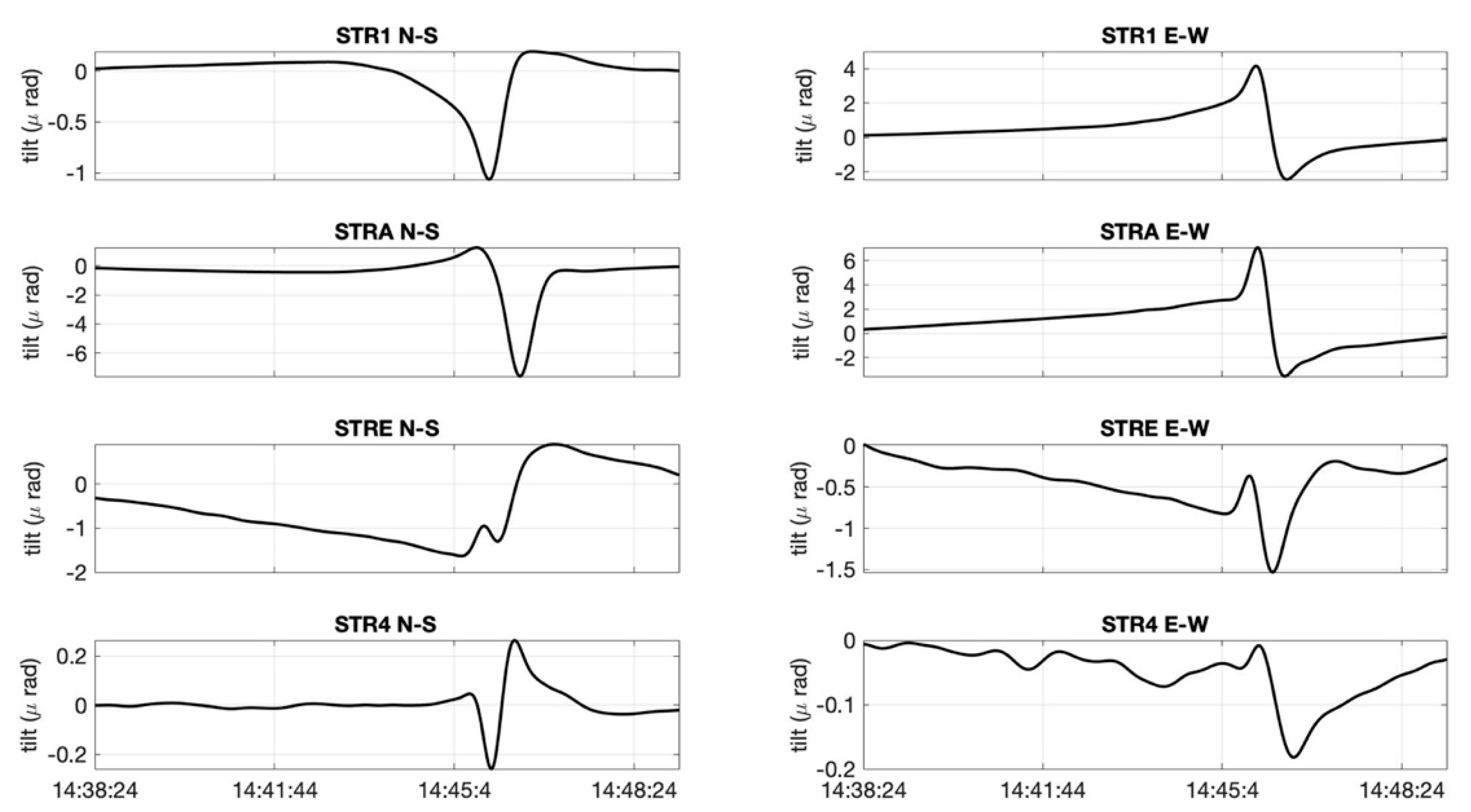
Appendix A.3.1. Tilt Data

Tilt has been continuously monitored at Stromboli since 1992 when three tilt stations (Figure 2) were installed at Punta Labronzo (PLB), Timpone Del Fuoco (TDF) beyond the southern and northern rims of the SdF (Sciara del Fuoco) and Punta Lena (PLN) using AGI Mod 722 borehole tiltmeters positioned about 3 m deep [41].
Between 2008 and 2010, two deep stations (−27 m) were installed at TDF and SVO (San Vincenzo) and equipped with high resolution (<0.005 μrad) and self-levelling instruments (AGI Lily). However, PLN and SVO soon showed severe site problems and, for this reason, only PLB and TDF (−27 m) are currently active. PLB and TDF are affected by low noise and their real precision is, respectively 0.04 and 0.01 μrad. Tilt data are transmitted in real-time to the INGV-OE building in Catania, including the two tilt components, and air and ground temperatures [12,42].
Figure A4. Tilt signals recorded at PLB and TDF stations in the period June 2018–August 2019. PLB Radial (tilt_x) is oriented toward the summit craters and positive variations indicate a crater uplift; PLB Tangential (tilt_y) is 90° counter-clockwise. TDF tilt_x is N275°E oriented (tilt_y is N185°E) and positive values indicate a downward tilt.
Remotesensing 13 04064 g0a4

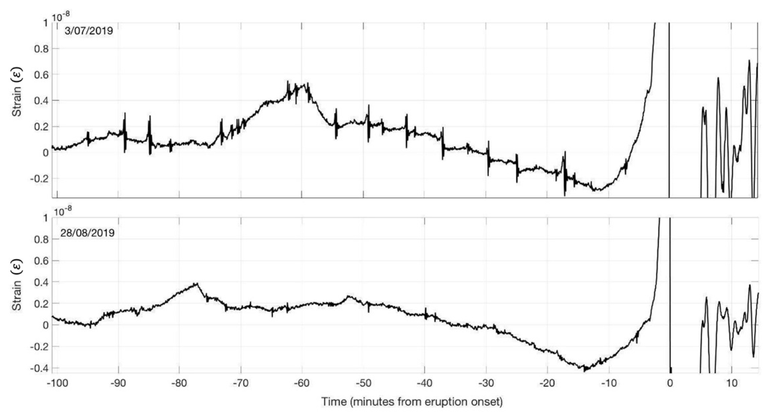
Appendix A.3.2. Dilatometric Data

Two borehole strainmeters were installed at Stromboli during 2006, with the support of the Italian Civil Protection Department, INGV, Università degli Studi di Salerno (Italy) and the Carnegie Institution of Washington D.C. (USA), located, respectively at Stromboli (SVO strainmeter, Figure 2) and Ginostra (TDF strainmeter, Figure 2), by drilling a borehole down to 120 m depth. The TDF instrument is not well coupled with the surrounding rocks; hence, in this paper, only SVO strain data have been analysed.
The Sacks-Evertson strainmeters (about 7 cm in diameter, 4 m in length) provide two signal outputs obtained by two different hydro-mechanical amplification systems with a nominal resolution of about 10−11 and a nominal dynamic range is 10−11–10−3. The borehole strainmeters are used to detect low frequency deformation transients but they are also capable of detecting elastodynamic deformation over a broad frequency range: at seismic frequencies, their performance characteristics are comparable to traditional seismometers [43,44].
From a visual inspection of the strain data filtered in 2–50 s frequency band, we obtained two principal families, each one characterized by a peculiar shape as described in the principal manuscript. In Figure A5, we reported the VLP daily occurrence rate from June 2018 to December 2019 in order to show that the 3 July paroxysm is the only explosive volcanic event preceded by a net increase in two families.
Figure A5. Histogram of the occurrence of VLPs belonging to the two families 1 and 2 starting from June 2018 until the end of year 2019. The solid red lines indicate the two major explosions that took place before the beginning of the paroxysmal activity. The dash-dotted red lines indicate the two 2019 paroxysms.
Remotesensing 13 04064 g0a5
Another feature emerges when strain data are observed a few minutes before the onset of the paroxysmal explosions: after each strain VLP a small strain drop occurs, leaving a slight temporary strain decrease (Figure A6).
Figure A6. Comparison of the last 100 min’ strain data recorded by the SVO strainmeter before the two paroxysmal eruptions of July and August 2019, showing the sudden and fast strain increase starting about 10 min before the paroxysms’ occurrence. The July eruption (upper panel) is characterized by a higher number of more energetic strain VLPs, each followed by a low strain drop.
Remotesensing 13 04064 g0a6

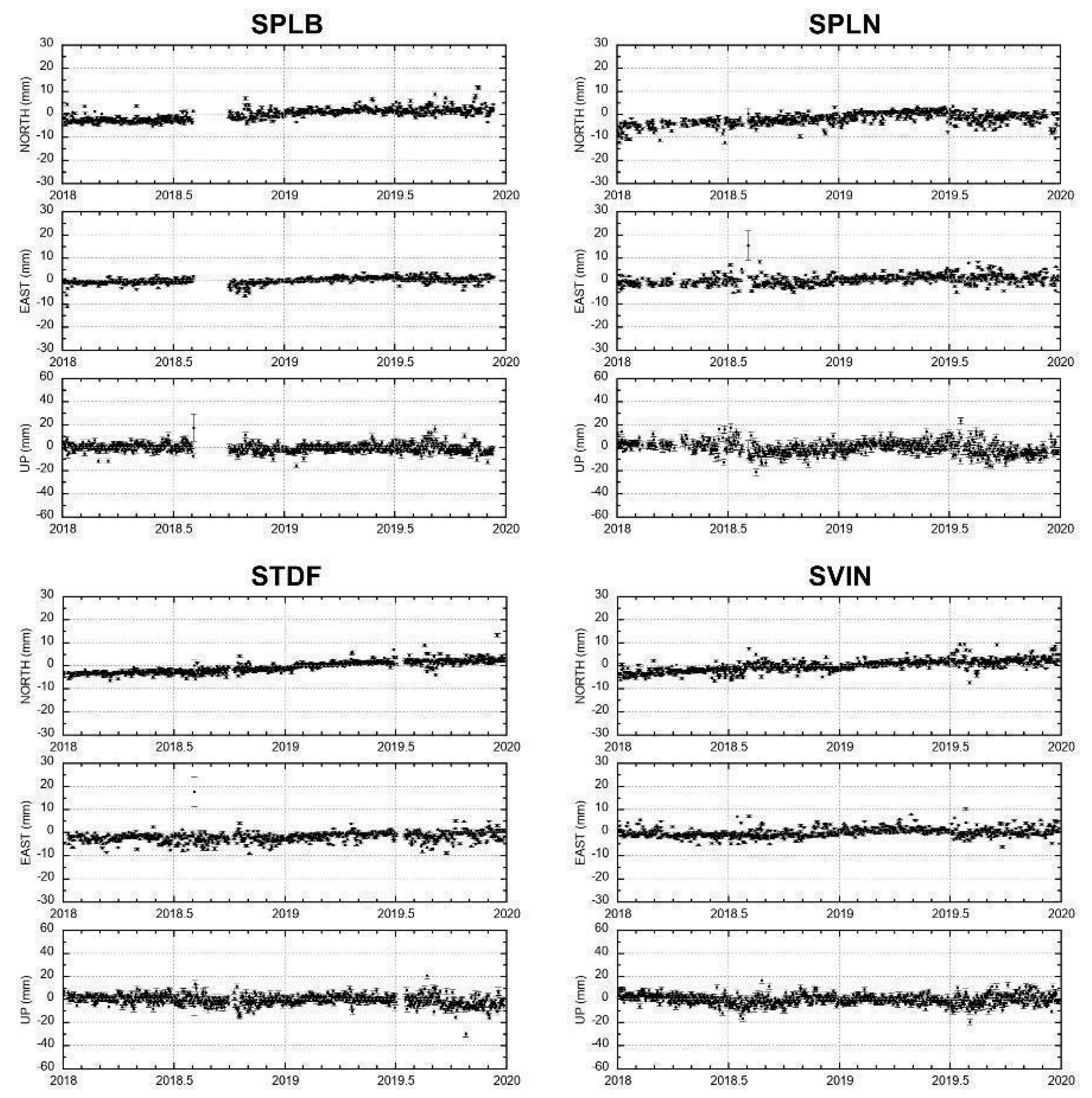
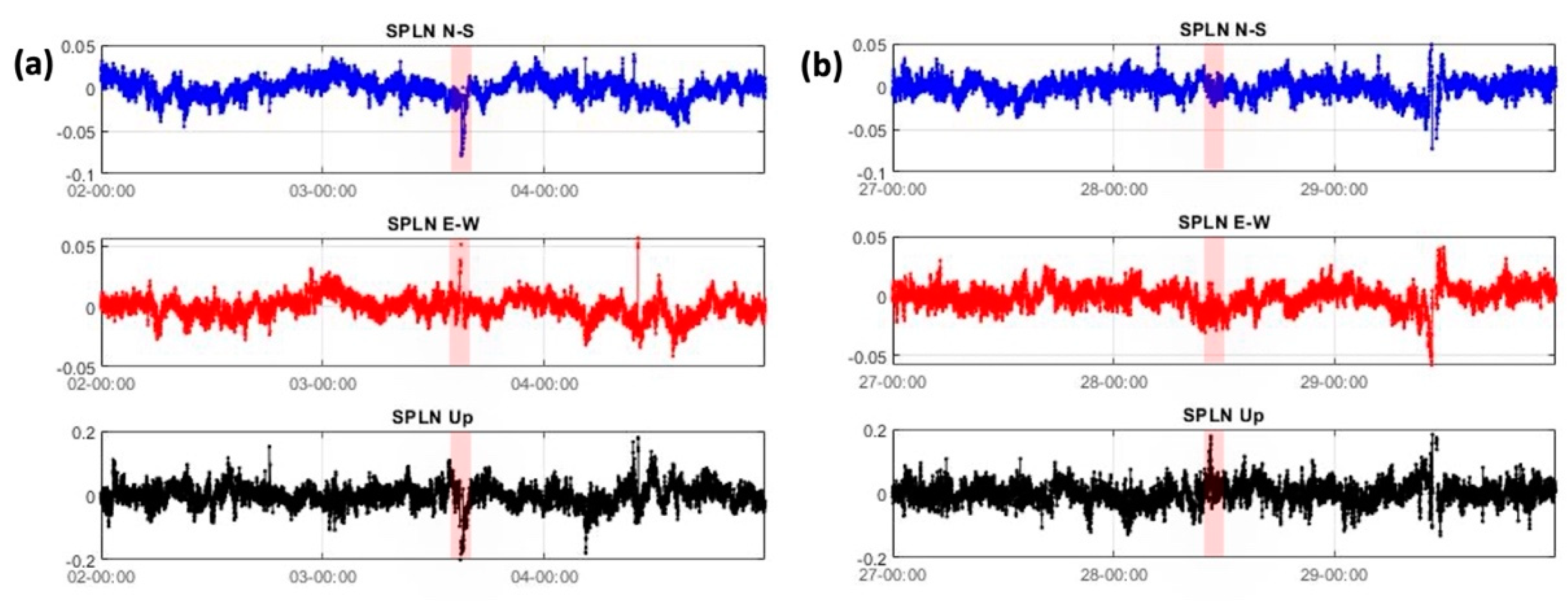
Appendix A.3.3. GNSS Data

Since 1997, four Continuous GPS (CGPS) stations operated at Stromboli volcano by the INGV-OE (Istituto Nazionale di Geofisica e Vulcanologia, Osservatorio Etneo) (Figure 2) have provided information about the spatial and temporal evolution of volcanic sources beneath the volcano [41,45].
In 2003, three additional CGPS stations were installed in the Sciara del Fuoco (Figure 2), with the aim of monitoring the potential catastrophic failure of the steep slope, but their lifespan was very short as they were destroyed by a paroxysm on 5 April 2003 [45]. The change in receivers and antennas that occurred between 2010 and 2018 marks the transition from a CGPS to a GNSS network.
The GNSS data processing is performed in static mode and on a daily basis by the Bernesetm GPS software v.5.0 [46] using the International GNSS Service (IGS) products. The IGS absolute phase centre corrections are applied. Independent baselines are selected considering the criterion of maximum common observations. The ambiguity resolution is based on the Quasi Ionosphere Free strategy. The troposphere delay is modelled using the dry-Niell a priori model and the troposphere zenith delay parameters were estimated every hour at each site using the wet-Niell mapping function. The geodetic datum is realized by three No-Net Translation conditions imposed on a set of eight IGS14 [47] reference stations (minimum constraint solution), which are included in the processing. In Figure A7, the daily time series of the Stromboli GNSS network are shown from January 2018 to December 2019. The Eurasian plate motion has been removed from the horizontal components (North and East) of the time series using Euler pole parameters in [48].
Figure A7. Daily time series of the four GNSS stations on Stromboli from January 2018 to December 2019. Horizontal components (NS and EW) in a fixed Eurasian reference frame.
Remotesensing 13 04064 g0a7
The HRGNSS (High Rate GNSS) data were processed with the method of instantaneous GPS positioning, already applied to volcano monitoring of Stromboli [45], Mt.Etna [49] and to study the 2005–2006 Mt. Augustine (Alaska) eruption [50]. We used the Geodetics RTDtm and RTKLIB ver. 2.4.2 (RTKLIB, an open source program package for GNSS positioning, http://www.rtklib.com, accessed on 30 September 2021).
Geodetics RTDtm is a software that provides independent relative position estimates at each observation epoch, by resolving integer-cycle phase ambiguities anew for each epoch. The instantaneous positions of the continuous stations were computed relative to the station SVIN. We used Geodetics RTDtm to process 1 Hz GNSS data and, in particular, to analyse the three-day time span crossing the two paroxysms of 3 July and 28 August (Figure A8a,b).
We also tested the RTKLIB software. We used the post-processing application program RTKPOST to obtain station positions every 30 s for a greater timespan (from 01/01/2019 to 31/12/2019) than was previously done with Geodetics RTDtm. RTKPOST implements a relative positioning algorithm based on a Kalman filter and a double-differencing technique and it employs LAMBDA and MLAMBDA strategies [51] for integer ambiguity resolution [52,53]. In the RTKPOST, the following processing options were chosen: Combined solution (Forward & Backward), Ionosphere free (L3), Saastamoinen tropospheric model, IGS final orbits, Continuous ambiguity resolution method and Satellite and receiver antenna model IGS14.ATX. We selected SVIN station as the reference station.
Figure A8. High rate 1 Hz N–S, E–W and Up components of SPLN GNSS station spanning 02/07/2019 to 04/07/2019 (a) and 27/08/2019 to 29/08/2019 (b) processed using RTDtm software. The 1 Hz data have been resampled using a median of 5 min and inter quartile range (IQR) filtered to cut outliers. Red rectangles indicate paroxysm occurrence.
Remotesensing 13 04064 g0a8

Appendix A.4. Modelling of Volcanic Sources

As previously mentioned, on the early afternoon of 3 July 2019, starting from ~14:40 UT, the borehole instruments, both strainmeter and tiltmeters highlighted significant common variations in the signals preceding the beginning of the paroxysmal phenomenon by about four minutes. On the contrary, the real-time GNSS network (Figure A7) did not record significant displacements just before the explosion, but exclusively at the beginning of the eruption. Using an analytical approach, we modelled the variations observed at one strainmeter (SVO) and at two tiltmeters (TDF and PLB) during the five minutes preceding the explosion from 14:40:00 to 14:45:30 UT. Moreover, using the method described in Lyons et al. [54] we deduced the corresponding tilt variations from the signals recorded at four seismic stations (STR1, STRA, STRE and STR4) located in the higher flanks of the volcano (Figure A9). We also used these tilt variations to better constrain the pressure source. Maximum tilt variations were in the order of a few με. Finally, we set no variations at the four high-frequency GPS stations (SPLB, SPLN, STDF and SVIN) located on the lower flanks of the volcano. We performed an analytical inversion of tilt (TDF, PLB, STR1, STRA, STRE, STR4), strain (SVO) and displacement data (SPLB, SPLN, STDF and SVIN set to zero variations) using a pressurizing source embedded in a homogeneous half-space described as a simple spherical source [13]. We verified that this type of simple source model, compared to other analytical models available in the literature, showed a good trade-off between the number of degrees of freedom and the goodness of the obtained data fit. Mogi source [13] is described by four parameters: the coordinates “X”, “Y” and “Z” of the punctiform sphere centre and the volume variation “ΔV”. These parameters were estimated using the pattern search technique [55] jointly with the local genetic algorithm search [56]. The simultaneous inversion of different datasets was performed by minimizing the reduced chi-square statistic normalized for the number of stations for each kind of data. The obtained solution was further refined using a non-linear least squares optimization. Uncertainties of each parameter were estimated using a Jackknife re-sampling method [57]. A typical value of 0.25 was assumed for the Poisson ratio [58]. To take the first order of topographical effects into consideration, we also added the elevation station corrections to the model [15]. For more details about this method, see Cannavò [14].
Figure A9. The N–S, E–W components tilt variations from the signals recorded at four seismic stations STR1, STRA, STRE and STR4.
Remotesensing 13 04064 g0a9

References

  1. Pichavant, M.; Pompilio, M.; D’Oriano, C.; Di Carlo, I. The deep feeding system of Stromboli, Italy: Insights from a primitive golden pumice. Eur. J. Mineral. 2011, 23, 499–517. [Google Scholar] [CrossRef]
  2. Bevilacqua, A.; Bertagnini, A.; Pompilio, M.; Landi, P.; Del Carlo, P.; Di Roberto, A.; Aspinall, W.; Neri, A. Major explosions and paroxysms at Stromboli (Italy): A new historical catalog and temporal models of occurrence with uncertainty quantification. Sci. Rep. 2020, 10, 17357. [Google Scholar] [CrossRef]
  3. Viccaro, M.; Cannata, A.; Cannavò, F.; De Rosa, R.; Giuffrida, M.; Nicotra, E.; Petrelli, M.; Sacco, G. Shallow conduit dynamics fuel the unexpected paroxysms of Stromboli volcano during the summer 2019. Sci. Rep. 2021, 11, 266. [Google Scholar] [CrossRef]
  4. Giordano, G.; De Astis, G. The summer 2019 basaltic Vulcanian eruptions (paroxysms) of Stromboli. Bull. Volcanol. 2021, 83, 1–27. [Google Scholar] [CrossRef]
  5. Giudicepietro, F.; López, C.; Macedonio, G.; Alparone, S.; Bianco, F.; Calvari, S.; De Cesare, W.; Donne, D.D.; Di Lieto, B.; Esposito, A.M.; et al. Geophysical precursors of the July–August 2019 paroxysmal eruptive phase and their implications for Stromboli volcano (Italy) monitoring. Sci. Rep. 2020, 10, 10296. [Google Scholar] [CrossRef]
  6. Di Lieto, B.; Romano, P.; Scarpa, R.; Linde, A.T. Strain Signals Before and During Paroxysmal Activity at Stromboli Volcano, Italy. Geophys Res. Lett. 2020, 47. [Google Scholar] [CrossRef]
  7. Andronico, D.; Del Bello, E.; D’Oriano, C.; Landi, P.; Pardini, F.; Scarlato, P.; Vitturi, M.D.M.; Taddeucci, J.; Cristaldi, A.; Ciancitto, F.; et al. Uncovering the eruptive patterns of the 2019 double paroxysm eruption crisis of Stromboli volcano. Nat. Commun. 2021, 12, 1–14. [Google Scholar] [CrossRef] [PubMed]
  8. Ganci, G.; Vicari, A.; Fortuna, L.; Del Negro, C. The HOTSAT volcano monitoring system based on combined use of SEVIRI and MODIS multispectral data. Ann. Geophys. 2011, 54, 5. [Google Scholar] [CrossRef]
  9. Ganci, G.; Bilotta, G.; Cappello, A.; Herault, A.; Del Negro, C. HOTSAT: A multiplatform system for the thermal monitoring of volcanic activity using satellite data. Geol. Soc. Lond. Spéc. Publ. 2016, 426, 207–221. [Google Scholar] [CrossRef]
  10. Bos, M.S.; Fernandes, R.M.S.; Williams, S.D.P.; Bastos, L. Fast error analysis of continuous GNSS observations with missing data. J. Geod. 2013, 87, 351–360. [Google Scholar] [CrossRef] [Green Version]
  11. Chouet, B.; Dawson, P.; Ohminato, T.; Martini, M.; Saccorotti, G.; Giudicepietro, F.; De Luca, G.; Milana, G.; Scarpa, R. Source mechanisms of explosions at Stromboli Volcano, Italy, determined from moment-tensor inversions of very-long-period data. J. Geophys. Res. Space Phys. 2003, 108, B1. [Google Scholar] [CrossRef]
  12. Gambino, S.; Falzone, G.; Ferro, A.; Laudani, G. Volcanic processes detected by tiltmeters: A review of experience on Sicilian volcanoes. J. Volcanol. Geotherm. Res. 2014, 271, 43–54. [Google Scholar] [CrossRef]
  13. Mogi, K. Relations between the eruptions of various volcanoes and the deformations of the ground surfaces around them. Bull. Earthquake Res. Inst. 1958, 36, 99–134. [Google Scholar]
  14. Cannavò, F. A new user-friendly tool for rapid modelling of ground deformation. Comput. Geosci. 2019, 128, 60–69. [Google Scholar] [CrossRef]
  15. Williams, C.; Wadge, G. An accurate and efficient method for including the effects of topography in three-dimensional elastic models of ground deformation with applications to radar interferometry. J. Geophys. Res. Space Phys. 2000, 105, 8103–8120. [Google Scholar] [CrossRef]
  16. Segall, P. Magma chambers: What we can, and cannot, learn from volcano geodesy. Philos. Trans. R. Soc. A Math. Phys. Eng. Sci. 2019, 377, 20180158. [Google Scholar] [CrossRef] [Green Version]
  17. Jaupart, C.; Vergniolle, S. Laboratory models of Hawaiian and Strombolian eruptions. Nat. Cell Biol. 1988, 331, 58–60. [Google Scholar] [CrossRef]
  18. Jaupart, C.; Vergniolle, S. The generation and collapse of a foam layer at the roof of a basaltic magma chamber. J. Fluid Mech. 1989, 203, 347–380. [Google Scholar] [CrossRef]
  19. Lane, S.J.; Chouet, B.A.; Phillips, J.C.; Dawson, P.; Ryan, G.A.; Hurst, E. Experimental observations of pressure oscillations and flow regimes in an analogue volcanic system. J. Geophys. Res. Space Phys. 2001, 106, 6461–6476. [Google Scholar] [CrossRef] [Green Version]
  20. Oppenheimer, J.; Capponi, A.; Cashman, K.; Lane, S.; Rust, A.; James, M. Analogue experiments on the rise of large bubbles through a solids-rich suspension: A “weak plug” model for Strombolian eruptions. Earth Planet. Sci. Lett. 2020, 531, 115931. [Google Scholar] [CrossRef]
  21. Caracciolo, A.; Gurioli, L.; Marianelli, P.; Bernard, J.; Harris, A. Textural and chemical features of a “soft” plug emitted during Strombolian explosions: A case study from Stromboli volcano. Earth Planet. Sci. Lett. 2021, 559, 116761. [Google Scholar] [CrossRef]
  22. Ferlito, C. Mount Etna volcano (Italy). Just a giant hot spring! Earth-Sci. Rev. 2018, 177, 14–23. [Google Scholar] [CrossRef]
  23. Ferlito, C.; Bruno, V.; Salerno, G.G.; Caltabiano, T.; Scandura, D.; Mattia, M.; Coltorti, M. Dome-like behaviour at Mt. Etna: The case of the 28 December 2014 South East Crater paroxysm. Sci. Rep. 2017, 7, 1–12. [Google Scholar] [CrossRef]
  24. Inguaggiato, S.; Vita, F.; Cangemi, M.; Calderone, L. Changes in CO2 Soil Degassing Style as a Possible Precursor to Volcanic Activity: The 2019 Case of Stromboli Paroxysmal Eruptions. Appl. Sci. 2020, 10, 4757. [Google Scholar] [CrossRef]
  25. Inguaggiato, S.; Vita, F.; Cangemi, M.; Inguaggiato, C.; Calderone, L. The Monitoring of CO2 Soil Degassing as Indicator of Increasing Volcanic Activity: The Paroxysmal Activity at Stromboli Volcano in 2019–2021. Geoscience 2021, 11, 169. [Google Scholar] [CrossRef]
  26. Ripepe, M.; Ciliberto, S.; Della Schiava, M. Time constraints for modeling source dynamics of volcanic explosions at Stromboli. J. Geophys. Res. Space Phys. 2001, 106, 8713–8727. [Google Scholar] [CrossRef]
  27. Esposito, A.M.; Giudicepietro, F.; D’Auria, L.; Scarpetta, S.; Martini, M.G.; Coltelli, M.; Marinaro, M. Unsupervised Neural Analysis of Very-Long-Period Events at Stromboli Volcano Using the Self-Organizing Maps. Bull. Seism. Soc. Am. 2008, 98, 2449–2459. [Google Scholar] [CrossRef]
  28. Dawson, P.; Chouet, B. Characterization of very-long-period seismicity accompanying summit activity at Kīlauea Volcano, Hawai’i: 2007–2013. J. Volcanol. Geotherm. Res. 2014, 278–279, 59–85. [Google Scholar] [CrossRef] [Green Version]
  29. Ripepe, M.; Pistolesi, M.; Coppola, D.; Donne, D.D.; Genco, R.; Lacanna, G.; Laiolo, M.; Marchetti, E.; Ulivieri, G.; Valade, S. Forecasting Effusive Dynamics and Decompression Rates by Magmastatic Model at Open-vent Volcanoes. Sci. Rep. 2017, 7, 3885. [Google Scholar] [CrossRef]
  30. Chouet, B. Dynamics of a fluid-driven crack in three dimensions by the finite difference method. J. Geophys. Res. Space Phys. 1986, 91, 13967–13992. [Google Scholar] [CrossRef]
  31. Chouet, B. Resonance of a fluid-driven crack: Radiation properties and implications for the source of long-period events and harmonic tremor. J. Geophys. Res. Space Phys. 1988, 93, 4375–4400. [Google Scholar] [CrossRef]
  32. Chouet, B. A Seismic Model for the Source of Long-Period Events and Harmonic Tremor. In IAVCEI Proceedings in Volcanology; Springer Gabler: Wiesbaden, Germany, 1992; pp. 133–156. [Google Scholar]
  33. Ohminato, T.; Chouet, B.; Dawson, P.; Kedar, S. Waveform inversion of very long period impulsive signals associated with magmatic injection beneath Kilauea volcano, Hawaii. J. Geophys. Res. Space Phys. 1998, 103, 23839–23862. [Google Scholar] [CrossRef]
  34. Chouet, B.; Dawson, P.; Arciniega-Ceballos, A. Source mechanism of Vulcanian degassing at Popocatépetl Volcano, Mexico, determined from waveform inversions of very long period signals. J. Geophys. Res. Space Phys. 2005, 110. [Google Scholar] [CrossRef] [Green Version]
  35. Ramsey, M.S.; Harris, A.J. Volcanology 2020: How will thermal remote sensing of volcanic surface activity evolve over the next decade? J. Volcanol. Geotherm. Res. 2013, 249, 217–233. [Google Scholar] [CrossRef]
  36. Ganci, G.; Vicari, A.; Bonfiglio, S.; Gallo, G.; Del Negro, C. A texton-based cloud detection algorithm for MSG-SEVIRI multispectral images. Geomatics Nat. Hazards Risk 2011, 2, 279–290. [Google Scholar] [CrossRef]
  37. Ganci, G.; Cappello, A.; Bilotta, G.; Del Negro, C. How the variety of satellite remote sensing data over volcanoes can assist hazard monitoring efforts: The 2011 eruption of Nabro volcano. Remote Sens. Environ. 2020, 236, 111426. [Google Scholar] [CrossRef]
  38. Calvari, S.; Ganci, G.; Victoria, S.; Hernández, G.D.P.; Perez, N.M.; Barrancos, J.; Alfama, V.; Dionis, S.; Cabral, J.; Cardoso, N.; et al. Satellite and Ground Remote Sensing Techniques to Trace the Hidden Growth of a Lava Flow Field: The 2014–2015 Effusive Eruption at Fogo Volcano (Cape Verde). Remote Sens. 2018, 10, 1115. [Google Scholar] [CrossRef] [Green Version]
  39. Cappello, A.; Ganci, G.; Calvari, S.; Pérez, N.M.; Hernández, P.A.; Silva, S.V.; Cabral, J.; Del Negro, C. Lava flow hazard modeling during the 2014-2015 Fogo eruption, Cape Verde. J. Geophys. Res. Solid Earth 2016, 121, 2290–2303. [Google Scholar] [CrossRef] [Green Version]
  40. Spampinato, L.; Ganci, G.; Hernández, P.A.; Calvo, D.; Tedesco, D.; Pérez, N.M.; Calvari, S.; Del Negro, C.; Yalire, M.M. Thermal insights into the dynamics of Nyiragongo lava lake from ground and satellite measurements. J. Geophys. Res. Solid Earth 2013, 118, 5771–5784. [Google Scholar] [CrossRef]
  41. Mattia, M.; Aloisi, M.; Di Grazia, G.; Gambino, S.; Palano, M.; Bruno, V. Geophysical investigations of the plumbing system of Stromboli volcano (Aeolian Islands, Italy). J. Volcanol. Geotherm. Res. 2008, 176, 529–540. [Google Scholar] [CrossRef]
  42. Gambino, S.; Cammarata, L. Tilt measurements on volcanoes: More than a hundred years of recordings. Ital. J. Geosci. 2017, 136, 275–295. [Google Scholar] [CrossRef]
  43. Borcherdt, R.D.; Johnston, M.J.S.; Glassmoyer, G. On the use of volumetric strain meters to infer additional characteristics of short-period seismic radiation. Bull. Seism. Soc. Am. 1989, 79, 1006–1023. [Google Scholar]
  44. Barbour, A.; Agnew, D.C. Detection of Seismic Signals Using Seismometers and Strainmeters. Bull. Seism. Soc. Am. 2012, 102, 2484–2490. [Google Scholar] [CrossRef]
  45. Mattia, M.; Rossi, M.; Guglielmino, F.; Aloisi, M.; Bock, Y. The shallow plumbing system of Stromboli Island as imaged from 1 Hz instantaneous GPS positions. Geophys. Res. Lett. 2004, 31. [Google Scholar] [CrossRef] [Green Version]
  46. Dach, R.; Hugentobler, U.; Fridez, P.; Meindl, M. Bernese GPS Software, Version 5.0; Astronomical Institute, University of Bern: Bern, Switzerland, 2007. [Google Scholar]
  47. Altamimi, Z.; Rebischung, P.; Métivier, L.; Collilieux, X. ITRF2014: A new release of the International Terrestrial Reference Frame modeling nonlinear station motions. J. Geophys. Res. Solid Earth 2016, 121, 6109–6131. [Google Scholar] [CrossRef] [Green Version]
  48. Altamimi, Z.; Métivier, L.; Rebischung, P.; Rouby, H.; Collilieux, X. ITRF2014 plate motion model. Geophys. J. Int. 2017, 209, 1906–1912. [Google Scholar] [CrossRef]
  49. Mattia, M.; Bruno, V.; Montgomery-Brown, E.; Patanè, D.; Barberi, G.; Coltelli, M. Combined seismic and geodetic analysis before, during and after the 2018 Mt. Etna eruption. Geochem. Geophys. Geosystems 2020, 21. [Google Scholar] [CrossRef]
  50. Mattia, M.; Palano, M.; Aloisi, M.; Bruno, V.; Bock, Y. High rate GPS data on active volcanoes: An application to the 2005–2006 Mt. Augustine (Alaska, USA) eruption. Terra Nova 2008, 20, 134–140. [Google Scholar] [CrossRef]
  51. Teunissen, P.J.G. The least-squares ambiguity decorrelation adjustment: A method for fast GPS integer ambiguity estimation. J. Geod. 1995, 70, 65–82. [Google Scholar] [CrossRef]
  52. Takasu, T. RTKLIB: Open Source Program Package for RTK-GPS. In Proceedings of the FOSS4G, Tokyo, Japan, 2 November 2009. [Google Scholar]
  53. Takasu, T.; Yasuda, A. Development of the low-cost RTK-GPS receiver with an open source program package RTKLIB. Proceedings of International Symposium on GPS/GNSS, International Convention Center Jeju, Seogwipo, Korea, 4–6 November 2009. [Google Scholar]
  54. Lyons, J.J.; Waite, G.; Ichihara, M.; Lees, J. Tilt prior to explosions and the effect of topography on ultra-long-period seismic records at Fuego volcano, Guatemala. Geophys. Res. Lett. 2012, 39, 08305. [Google Scholar] [CrossRef]
  55. Lewis, R.M.; Torczon, V. Pattern Search Algorithms for Bound Constrained Minimization. SIAM J. Optim. 1999, 9, 1082–1099. [Google Scholar] [CrossRef]
  56. Goldberg, D.E. Genetic Algorithms in Search Optimization and Machine Learning; Addison-Wesley: Boston, MA, USA, 1989; 432p. [Google Scholar]
  57. Efron, B. The Jackknife, the Bootstrap and Other Resampling Plans; Stanford University Press: Stanford, CA, USA, 1982. [Google Scholar]
  58. Aloisi, M.; Mattia, M.; Monaco, C.; Pulvirenti, F. Magma, faults, and gravitational loading at Mount Etna: The 2002–2003 eruptive period. J. Geophys. Res. Space Phys. 2011, 116. [Google Scholar] [CrossRef]
Figure 1. (a) The paroxysm of 3 July 2019 (left) seen from the sea looking towards NE with Ginostra village in the foreground (photo by Fabrizio Schiano). (b) Thermal image, with rainbow palette colours (lighter colours represent higher temperatures), of the 28 August 2019 paroxysm. The hot cloud related to the pyroclastic flow along the Sciara del Fuoco, lower left, and the eruptive column are visible.
Remotesensing 13 04064 g001
Figure 2. Map of Stromboli Island with all the monitoring devices used in this work.
Remotesensing 13 04064 g002
Figure 3. (a) Total cumulative dispersion CD (north crater + south crater) moving average (49 samples; green line); one sample every hour (1135 samples). For times when the green line is interrupted there is no signal, since the camera was not working. The last sample was collected just before the 3 July paroxysm, when the camera was destroyed by the outburst. In orange, a possible threshold between “normal” and “potentially dangerous” activity. This threshold, being based on this dataset alone, must be considered only as an indication. Blue dots represent the MODIS-derived radiant heat flux measured at Stromboli. (b) The location of the explosive activity (intensity and position) is shown. Orange areas are the periods with prevalent explosive activity from the South crater while blue areas are the periods with prevalent activity from the north crater.
Remotesensing 13 04064 g003
Figure 4. (ac). Comparison between tiltmeter and strainmeter data (ac). Upper panels (a,b) show, respectively TDF and PLB tilt components recorded at one sample per minute; lower panel (c) shows SVO strain data recorded at one sample per second. PLB tilt-x is oriented toward the summit craters and positive variations indicate a crater uplift (radial); PLB tilt-y is 90° counter-clockwise (tangential). TDF tilt-x is N275°E oriented (TDF tilt-y is N185°E) and positive values indicate a downward tilt. Strainmeter data are filtered between 3 and 5000 s. Dashed line marks the 3 July eruption beginning (14:45:40 UTC). (d,e) Stromboli GNSS horizontal velocity field (2018–2019). The velocities are calculated in a fixed Eurasian reference frame (blue arrows in d) or considering the SVIN station as fixed (red arrows in e). (f) High rate GNSS data (30 s) of SPLN station spanning 01/06/2019 to 15/07/2019 processed epoch by epoch using RTKLIB software. The uplift of the station observed between 23 and 28 June may be related to volcanic input. The 30 s data (in grey) have been resampled using a median of 60 min (in black). The red line represents a median filter with a window size of 3 days every hour.
Remotesensing 13 04064 g004
Figure 5. Strain VLP parameters change as recorded by SVO strainmeter from June 2018 to December 2019. The evidenced area with a red rectangle shows changes occurring from the beginning of June until the July eruption. Top to bottom: (a) strain, filtered in 2–50 s frequency band; (b) peak-to-peak amplitude change; (c) intertime between VLPs; (d) duration of each strain VLP; (e) frequency change, averaged on periods comprised between 25 and 70 s; (f) occurrence of strain VLPs per day.
Remotesensing 13 04064 g005
Figure 6. (a) Stacking of strain VLP waveforms selected after a visual inspection. Family 1 and family 2 events are represented. (b) Stacked, normalized waveforms of seismic events of each of the six families in which seismic VLPs were grouped by means of cross-correlation analysis. (c) Daily occurrence rate of seismic VLP events grouped into the six families identified by means of cross-correlation. (d) Normalized stacking of waveforms belonging to family 1 in the time period 1–24 June (blue line) and 25 June–3 July (red line).
Remotesensing 13 04064 g006
Figure 7. (a,b) Model of the source acting during the 3 July 2019 paroxysm. The red sphere indicates the horizontal position (in a) and the depth (in b) of the source. Observed (blue lines) and modeled (red lines) tilt vectors are reported in a. The position and the dimension source values are: Long = 15.211° ((518,314 ± 5) m, UTM-WGS84); Lat = 38.792° ((4,293,780 ± 3) m, UTM-WGS84); Z = (+80 ± 0) m; ΔV = (10,478 ± 1206) m3. The “Z” parameter is reported with respect to sea level.
Remotesensing 13 04064 g007
Figure 8. Main signals from the INGV monitoring networks. Red and blue dashed lines mark the two explosive events. Yellow and blue filled rectangles represent, respectively the medium and the short pre-paroxysmal phases. Red filled rectangle represents eruptive phase. In this synthetic panel the comparison among all the data shows a convergence toward an unrest phase preceding the 3 July 2019 paroxysm.
Remotesensing 13 04064 g008
Figure 9. This panel shows a more focused view of the signals, indicating clear variations before the occurrence of the 3 July 2019 paroxysm. In particular, the synchrony of variations observed in seismic and strain VLP is more evident.
Remotesensing 13 04064 g009
Figure 10. Schematic picture of active source model during the paroxysm episode. (a) The feeding system during the “steady state” activity: the flux of WMS is regularly released through CMP without any significant increase in the WMS pressure. (b) The increase in the WMS flux causes a pressure increment, as well as an increment in the degassing at the crater level, thus bringing about a strong explosive activity. (c) When the flux increase of the WMS cannot be contained by the CMP the paroxysm occurs. The CMP is ejected by the pushing force of the WMS that is in turn ejected as well.
Remotesensing 13 04064 g010
Publisher’s Note: MDPI stays neutral with regard to jurisdictional claims in published maps and institutional affiliations.

