Multi-Space Seasonal Precipitation Prediction Model Applied to the Source Region of the Yangtze River, China

Abstract

This paper developed a multi-space prediction model for seasonal precipitation using a high-resolution grid dataset (0.5° × 0.5°) together with climate indices. The model is based on principal component analyses (PCA) and artificial neural networks (ANN). Trend analyses show that mean annual and seasonal precipitation in the area is increasing depending on spatial location. For this reason, a multi-space model is especially suited for prediction purposes. The PCA-ANN model was examined using a 64-grid mesh over the source region of the Yangtze River (SRYR) and was compared to a traditional multiple regression model with a three-fold cross-validation method. Seasonal precipitation anomalies (1961–2015) were converted using PCA into principal components. Hierarchical lag relationships between principal components and each potential predictor were identified by Spearman rank correlation analyses. The performance was compared to observed precipitation and evaluated using mean absolute error, root mean squared error, and correlation coefficient. The proposed PCA-ANN model provides accurate seasonal precipitation prediction that is better than traditional regression techniques. The prediction results displayed good agreement with observations for all seasons with correlation coefficients in excess of 0.6 for all spatial locations.

1. Introduction

Precipitation is an important resource that affects ecological health, agricultural yield, and economic growth. Thus, the ability to predict future precipitation anomalies has received considerable research attention [1,2,3,4,5]. Predictive models can help decisionmakers to better manage finite future water resources. The source region of the Yangtze River (SRYR), the origin of the longest river in China, is located in the central Tibet Plateau. With occurring wetland degradation and biodiversity reduction, the variability of precipitation has a significant influence on the sustainability of the basin itself and downstream areas [6,7]. Thus, the ability to predict future precipitation in this area is of great importance.

To improve the prediction skill of precipitation in the SRYR, it is important to improve the physical understanding and mapping of relationships between regional climate and local precipitation. During recent years, researchers have made significant progress in this respect by introducing associations with external forcing of atmospheric circulation patterns (teleconnections). Numerous studies worldwide have shown that teleconnections have a strong impact on present and future precipitation. Examples of such teleconnection indices are El Niño–Southern Oscillation (ENSO), Pacific Decadal Oscillation (PDO), North Atlantic Oscillation (NAO), West Pacific pattern (WP), Polar Eurasian pattern (POL), Pacific/North American (PNA) Pattern, and Scandinavia Pattern (SCA). These indices have been linked to interannual/interdecadal boreal precipitation variability [2,5,8,9,10,11,12,13,14].

For major catchments in China, regression models have been an initial choice for precipitation prediction. Chan and Shi [15] derived a statistical regression model for forecasting the summer monsoon rainfall over South China using indices that serve as proxies for ENSO and planetary-scale circulation. The region was first mapped into three subregions by applying cluster analyses. Predictands were set as average precipitation over the different subregions. Kim and Kim [16] applied linear regression to predict precipitation in China with adaptive predictors from regularly updated climate indices and two to twelve-month lead-time. Considering the complex interactions between predictors and the outcome, artificial neural network (ANN) models are preferred over traditional regression models since they can address problems involving nonlinear interactions without prior knowledge. Hartmann, Becker [17] predicted summer rainfall in the Yangtze River Basin with neural networks, using indices of winter sea surface temperature and sea level pressure. The outcome of the neural network was summer rainfall from May to September that was classified into six different subregions. Yuan, Berndtsson [18] predicted summer precipitation for the source region of Yellow River using an ANN model, in which a back-propagation neural network was developed using significantly correlated climate indices.

In all the above studies, methods were used to deal with spatial variability of precipitation anomalies of the study area (subregion division). By dividing stations into different homogenous regions, the average precipitation will represent stations in the same subregion that can be used as predictands. It is an efficient method, especially for large basins with significant spatial variation. The disadvantage is that part of the variability in the dataset might be lost.

Another common problem in the above studies was that the prediction for different subregions used static parameters, which ignored the spatial differences between teleconnections and subregions. Moreover, different climate indices with different time lags will affect precipitation variation at a fine spatial resolution. Previous studies have not addressed this issue in a comprehensive manner. A better understanding of these relationships can improve the prediction skill of spatial precipitation [19]. Thus, adaptive and spatially distributed predictors should be used to optimize prediction results.

In view of the above, the objective of this study was to fill research gaps regarding precipitation prediction and the relationship with climate indices for the SRYR. We introduced a multi-space model for seasonal precipitation prediction by applying PCA and ANN techniques. Accordingly, this paper assessed the ability of the PCA-ANN model to provide an accurate prediction of seasonal precipitation considering spatial variation. A newly presented grid precipitation dataset (0.5° × 0.5°, updated to 2015) was used to represent the spatiotemporal variability of precipitation, including trend at the annual/seasonal scale. The developed spatiotemporal model used selected climate indices as predictors. The performance of the model was evaluated by comparison with a multiple linear regression model (MLR).

2. Study Area and Data

The SRYR is located in the hinterland of the Qinghai-Tibet plateau, which refers to the area above the Zhimenda runoff station (Figure 1). The region has an average elevation of over 4500 m amsl (90°33′–95°20′ E, 32°26′–35°46′ N), and the area is approximately 13.77 × 10⁴ km². More than 200 small tributaries contribute to the runoff in the source region and discharge from Zhimenda runoff station into the downstream basin. Based on the Köppen Geiger climate classification system [20], the SRYR is characterized by a monsoon-influenced subarctic climate (Dwc), which means dry winters and cool summers.

Gridded data (0.5° × 0.5°), spatially interpolated from monthly precipitation for the period 1961–2015 over China, were obtained from the China Meteorological Administration (CMA). Precipitation data over the SRYR were extracted based on a mask (Figure 1). The gridded data were created by CMA based on all available precipitation data at 2472 stations and a digital elevation model from GTOPO30. The thin plate spline method was used to interpolate precipitation into 0.5° × 0.5° grids using longitude, latitude, and altitude [21]. The data quality was previously checked by Zhao, Zhu [22] using cross-validation and error analysis. The data have been widely used in climate analysis, numerical model verification, and hydrological studies [23,24].

Seasonal precipitation data for each grid in Figure 1 were calculated based on the monthly time series. The arithmetic average of all gridded monthly mean data during the study period was used for the basin-scale assessment. The calendar-based year (January–December) and climatological seasons (March-April-May (MAM) representing spring; June-July-August (JJA) summer; September-October-November (SON) autumn; December-January-February (DJF) winter) were used in this study as annual and seasonal time scales. To calculate the correlation between climate indices and precipitation, seasonal precipitation anomalies were standardized by division with the standard deviation.

To describe modes of atmospheric circulation, this study considered six climate indices influencing climate variability over the Northern Hemisphere, and especially China: Southern Oscillation Index (SOI), Pacific Decadal Oscillation (PDO), North Atlantic Oscillation (NAO), Pacific/North American (PNA) Pattern, Scandinavia Pattern (SCA), and Polar/Eurasia Pattern (POL). Standardized monthly data of climate indices are available from the Climate Prediction Centre (CPC) at the National Weather Service of the United States (http://www.cpc.ncep.noaa.gov/data/teledoc/telecontents.shtml). This study used monthly data for the period of January 1961 to December 2015, which are available online. The seasonal data of climate indices were calculated as the average of monthly data for the climatological seasons. A further explanation of each climate index is given by Barnston and Livezey [25] and Washington, Hodson [26].

3. Methods

3.1. Linear Trend Analysis

To investigate precipitation trend and variability in the SRYR, seasonal precipitation time series from 1961 to 2015 for all grids were examined using linear regression [27] and the nonparametric Mann–Kendall test. The gradient for a long-term changing trend y was estimated as:

$$\frac{dy\left(t\right)}{dt}=a_1$$

(1)

where a₁ is the linear hydro-climatic trend over a year. The sum of squared residuals (difference between observations and fits) was minimized to estimate a₁.

3.2. Design of the PCA-ANN Model

The PCA-ANN model is a combination of principal component analysis (PCA) and artificial neural network (ANN), by which principal components (PCs) of the original precipitation dataset were used as simulating targets for the ANN model. The step-by-step procedure of the PCA-ANN model is shown in Figure 2.

3.2.1. PCA Analysis

PCA analysis was first applied to the target dataset, seasonal precipitation anomalies. PCA results present complex data in a simplified way to identify relations between driving variables [28,29]. The R-mode PCA [30,31], which aims to reduce the complexity of the variables, was used in this study (data matrix with rows of years and columns for the 64 grids of seasonal precipitation anomalies). The number of leading modes to be retained for further analysis was decided based on a simple rule of thumb. Loadings of the modes are the spatial patterns corresponding to locations with high variability, and the associated scores are the temporal patterns related to these locations, also referred to as PCs. The PCA for the spatiotemporal field of precipitation P(s, t) is defined as:

$$\mathrm{P}\left(\mathrm{s},\mathrm{t}\right)={\displaystyle \sum }_{i=1}^{M}Scor{e}_i\left(t\right)·Loadin{g}_i\left(s\right)$$

(2)

where t and s denote the temporal and spatial pattern, respectively, and M is the number of modes retained.

By PCA analysis, the input variables (64 grids) were converted into mutually independent PCs. Meanwhile, the information of input variables was preserved in these PCs with a minimum loss. Using the leading PCs, reconstruction yielded a modified precipitation dataset with less noise. Therefore, using leading PCs as targets for the PCA-ANN model had several advantages for model simulation: The number of targets was reduced from 64 grids to 3 PCs, overfitting due to noise was reduced, and the similarity between each model was minimized.

3.2.2. Identification of Potential Predictors

Spearman’s rank correlation (rho) [32] was used to identify driving variables among different climate indices for precipitation, as it assumes no normality or other specific distribution functions for the variables. Correlation coefficients between climate indices and seasonal precipitation PCs were investigated for different lag times (zero to four seasons). Climate indices were considered to be potential predictors if the correlation coefficients were significant at the 0.05 significant level, and the lag time with highest correlation was selected.

3.2.3. Selection of Predicting Model

To confirm the ability of the ANN model to stimulate PCs, a traditional multiple linear regression (MLR) model was used for validation. The MLR model [33] is given by:

$$\widehat{y}\left(t_n\right)=a_0+a_1{x}_1\left(t_{n-\tau 1}\right)+\dots +a_i{x}_i\left(t_{n-\tau i}\right),$$

(3)

where $\widehat{y}\left(t_n\right)$ is the simulated precipitation anomaly, $x_i$ (i = 1, ..., I) is the potential predictor, $\tau i$ ≥ 0 is the lag time between precipitation anomaly and the ith predictor, and a_i is the regression model parameter. The a_i was estimated from the training period results. The least-squares method was employed to calibrate the parameters and a stepwise method [34] was used to further select qualified predictors from all potential predictors.

3.2.4. Apply ANN Model for Prediction

The ANN was used to map the qualified predictors (input) and predictable PCs (output). The ANN customary architecture is composed of three layers of neurons: Input, hidden, and output layer [35]. Development of an ANN model consists of the following procedure:

(1) Setting up a typical feed-forward neural network, as this has been shown to be computationally superior in comparison to other alternatives;

(2) rescaling all input and output variables to (−1, 1) using:

$$x=\frac{2\left(x-x_{\min }\right)}{(x_{\max }-x_{\min )}}-1,$$

(4)

where x is the variable, x_min is the variable minimum, and x_max is the variable maximum;

(3) dividing the dataset into training, validation, and test sets (training set = fit ANN model weights, validation = select model type that provides the best level of generalization, and test set = evaluate the chosen model against the remaining data);

(4) selecting the activation function to hidden and output layer and training algorithm that provides the best fit to the data;

(5) identifying the optimal number of neurons in the hidden layer using a trial and error procedure by varying the number of hidden neurons from 2 to 10;

(6) evaluating the ANN model with statistics for multicriteria assessment using mean absolute error (MAE), root mean squared error (RMSE), and correlation between observations and simulation results (R). ANN analyses were performed using the MATLAB Neural Network Toolbox.

3.2.5. Model Evaluation

When comparing performance between ANN and MLR models, a three-fold cross-validation technique was used. All samples were randomly divided into three complementary subsets: k₁ = 18, k₂ = 18, and k₃ = 19. Each unique subset was taken as a test set while the remaining two subsets were used as a training set. A model was trained on the training set and evaluated for the test set. The evaluation scores (MAE, RMSE, and R) were retained, and the model was discarded. To reduce variability, the evaluation results were averaged over the three rounds to provide an estimate of the model’s predictive performance. By comparing the performance, the best model was selected between the ANN and MLR models. The ANN models proved to be superior compared to the MLR models. Thus, the ANN was trained over the entire dataset to tune to the prediction model. The output from the ANN model was transferred to precipitation anomalies through the inverse transform of rescaled and reconstructed PCAs. The results yielded a simulated precipitation dataset over the entire basin, corresponding to 64 grid points. Prediction results were compared to the target dataset using MAE, RMSE, and R.

4. Results

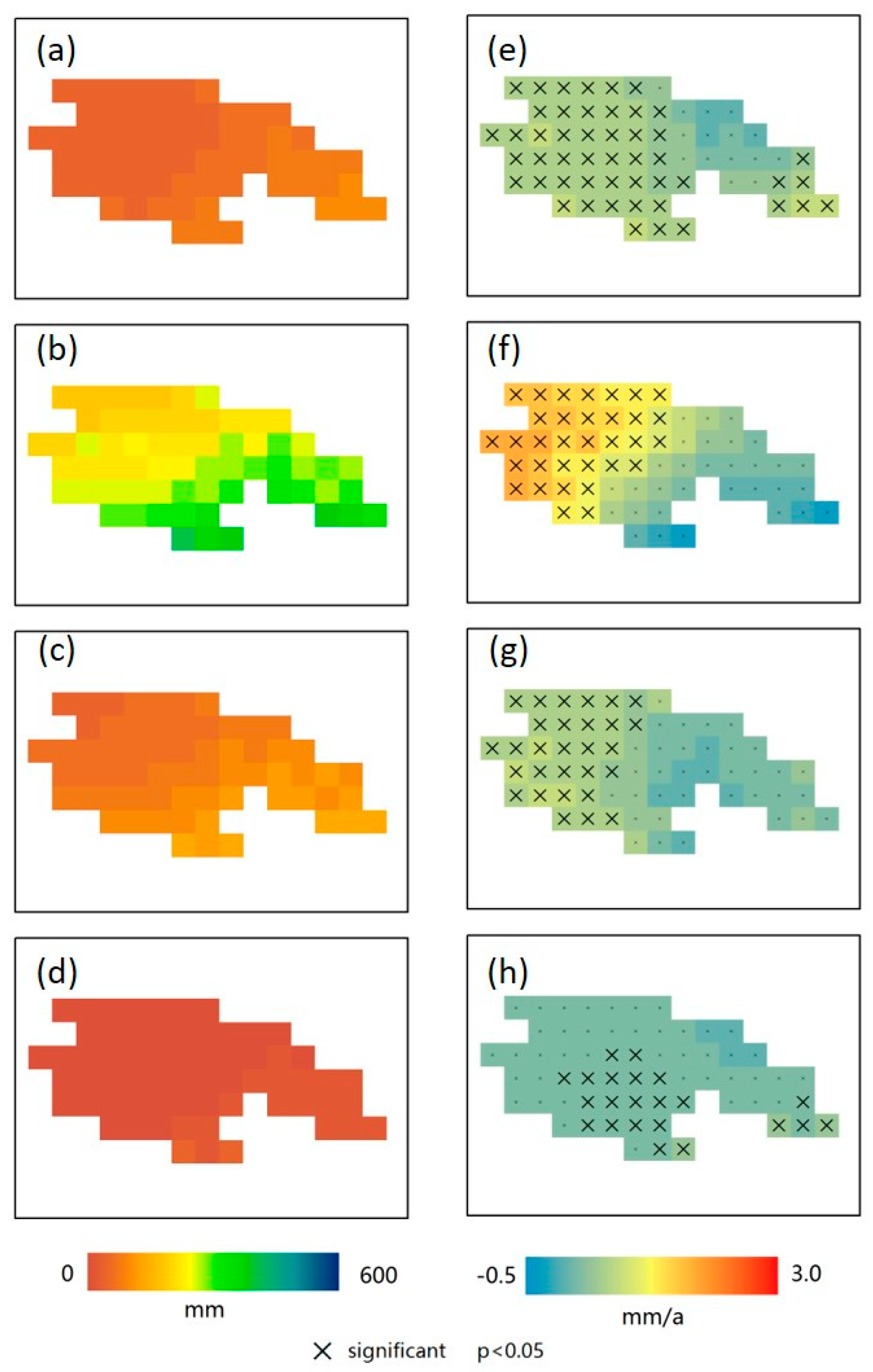
4.1. Precipitation Regime

Located on the Tibet Plateau, the SRYR precipitation showed high topographical dependence. The mean annual precipitation varied markedly over the basin. In general, there was larger precipitation in the southeastern areas that decreased toward the northwestern high elevation areas (from 632.6 to 234.6 mm; Figure 3a). This distribution stemmed from the southeasterly monsoon that weakened as it approached the inland. There was a significantly (p < 0.05) increasing trend in annual precipitation (warming) across the western part (Figure 3b). This trend equaled about 2.3 mm/year for the significant area of the basin.

Mean seasonal precipitation had an average range of 26.4 to 95.1 mm for spring (Figure 4a), 166.4 to 405.7 mm for summer (Figure 4b), 37.0 to 136.6 mm for autumn (Figure 4c), and 3.7 to 23.8 mm for winter (Figure 4d). In general, the largest precipitation for all seasons was observed over the south and southeast part of SRYR, while the driest areas were located in the northwestern parts. The seasonal precipitation for SRYR showed a very high variability during the period (1961–2015).

Trend analysis of seasonal mean precipitation showed both increasing and decreasing tendencies, but only increasing trend was statistically significant (p < 0.05). The significantly (p < 0.05) increasing trend in spring (Figure 4e) ranged from 0.3 to 0.7 mm per year and occurred over the western parts and in the eastern corner. During summer (Figure 4f), a statistically significant increasing trend (p < 0.05) only occurred over the western part, in the range of 0.8 to 1.9 mm per year. Autumn (Figure 4g) mean precipitation also showed a significant increase over the western part but with a smaller area than in summer. The general range of significantly increasing trend in autumn precipitation was between 0.3 and 0.7 mm per year. For winter (Figure 4h), mean precipitation displayed a significantly increasing trend (range 0.1 to 0.8 mm per year) over the central area and a small area in the southeast.

4.2. Predictor Evaluation

4.2.1. Principal Component Analysis (PCA)

PCs for the original precipitation dataset were used as simulating targets instead of the original data. In this way, the number of targets was reduced from 64 grids to three PCs, and overfitting was avoided since noise was filtered out. The similarity between each model was minimized because PCs are uncorrelated. Thus, time series at 64 grids over the basin for seasonal precipitation anomalies were subjected to PCA. The leading three PCs for different seasons explained about 91%, 92%, 90%, and 87% (

Table 1. Explained variance of leading principal components (PCs) for seasonal precipitation.

%	PC1	PC2	PC3	Cumulative
MAM	71.4	11.2	8.1	90.7
JJA	64.3	19.6	8.5	92.4
SON	65.6	15.4	9.2	90.2
DJF	63.1	14.0	10.0	87.1

) of the total variance, respectively. These were retained for further analysis.

Spatial patterns of these three PCs are illustrated in Figure 5. The first PC for MAM, JJA, SON, and DJF has high loading for grids covering the entire SRYR (Figure 5(a₁,b₁,c₁,d₁), which shows variation affecting the region as a whole with maximum loadings in the center of the basin, and hence represents rainfall events common for all grids. This PC represents the most important component of the total precipitation variance, with an explained variance of about 71%, 64%1 66%, and 63%, respectively (Table 1). All variables exhibited positive correlations with the first PC. By projecting precipitation anomalies onto PC1, time series representing the most important precipitation variance were retained that can be analyzed together with climate indices.

The second PCs have opposite loadings for the grids in west–east direction (Figure 5(a₂,b₂,c₂,d₂)), with explained variance of about 11%, 20%, 15%, and 14%, respectively (Table 1), indicating that the second most important precipitation variance has opposite variability over the western and eastern part. The zero line between negative and positive loadings extends from northern to the southern part of the basin. The zero line can be interpreted as dividing the basin into two parts: Reduced continental influence (or maritime influence, positive loadings) and strong continental influence (negative loadings). In spring, autumn, and winter, the zero line lies almost straight along the center, while in summer, the zero line leans toward the western part, which covers a larger area with positive loadings. This suggests that strengthening the summer monsoon brings moisture from the Pacific Ocean further into the west part of the basin.

Similarly, the third PC has opposite loadings for grids in the north–south direction (Figure 5(a₃,b₃,c₃,d₃), with an explained variance of about 8%, 9%, 9%, and 10%, respectively (Table 1). The zero line separates the north of the basin from the south and leans more toward the north side in the western part and more toward the south side in the eastern part. This division is due to topographic effects. As the southwestern part is the highest area of the basin, elevation reduces gradually from the southwest to the east (Figure 1). Topography plays an important role when winds bring moisture from the southeast and the Indian Ocean [36].

According to this analysis, spatial variability was retained by principal components that can be used for predictive purposes.

4.2.2. Correlation with Climate Indices

Spearman rank correlation (rho) was calculated to reveal the association between climate indices and spatial PCs. In order to consider nonlinear relationships between regional climate indices and local precipitation, correlation analyses were conducted for both concurrent and lagged time periods. Changing climate indices were assumed to give changes for present or future precipitation patterns.

In spring, the significantly influencing indices for PC1 were NAO, SOI, and POL (

Table 2. Spearman rank correlation between climate indices and leading PCs.

Season	PC	Lag 0						Lag 1
		NAO	PNA	SOI	PDO	SCA	POL	NAO	PNA	SOI	PDO	SCA	POL
MAM	PC1	0.363	---	0.230	---	---	−0.371	---	---	0.312	---	---	---
	PC2	---	---	---	---	---	---	---	---	---	---	---	---
	PC3	0.238	---	−0.391	0.377	0.459	---	---	0.306	−0.450	0.312	---	---
JJA	PC1	−0.274	---	---	---	---	---	---	---	---	−0.302	---	---
	PC2	---	---	---	---	---	---	---	---	---	---	0.342	---
	PC3	---	---	---	---	---	0.456	---	---	---	---	---	---
SON	PC1	---	---	---	---	---	---	---	---	---	---	---	0.275
	PC2	---	---	---	---	---	---	---	---	---	−0.266	---	---
	PC3	---	---	---	---	---	---	---	---	---	---	---	---
DJF	PC1	0.421	0.248	---	---	−0.388	---	---	---	---	---	---	---
	PC2	---	---	---	---	---	---	---	---	---	---	---	−0.271
	PC3	-0.231	---	---	---	---	---	---	---	---	---	---	---
Season	PC	Lag 2						Lag 3
		NAO	PNA	SOI	PDO	SCA	POL	NAO	PNA	SOI	PDO	SCA	POL
MAM	PC1	---	---	0.305	---	---	---	−0.352	---	---	---	---	---
	PC2	---	---	---	---	---	---	---	---	---	---	---	---
	PC3	---	---	−0.464	0.396	---	---	---	---	−0.262	0.243	---	---
JJA	PC1	---	---	0.365	−0.282	---	---	---	---	0.366	−0.270	---	---
	PC2	---	---	−0.250	---	---	---	---	---	−0.229	---	---	---
	PC3	---	---	---	---	---	---	---	---	---	---	---	---
SON	PC1	---	---	---	---	---	---	---	---	---	---	---	---
	PC2	---	---	0.305	−0.360	---	---	---	---	0.297	−0.335	---	---
	PC3	---	---	---	---	---	---	---	---	---	---	---	---
DJF	PC1	---	---	−0.236	0.298	---	---	0.273	---	---	0.371	---	−0.254
	PC2	---	---	---	---	---	---	---	---	---	---	---	---
	PC3	---	---	---	---	0.236	---	---	---	---	---	---	---
Season	PC	Lag 4
		NAO	PNA	SOI	PDO	SCA	POL
MAM	PC1	---	---	---	---	---	−0.278	Lag 0 = current quarter
	PC2	---	---	---	−0.254	---	---	Lag 1 = one quarter ahead
	PC3	---	---	---	---	---	0.253	Lag 2 = two quarters ahead
JJA	PC1	---	---	0.273	−0.261	---	---	Lag 3 = three quarters ahead
	PC2	---	0.270	---	---	---	---	Lag 4 = four quarters ahead
	PC3	---	---	---	---	---	---	Red background: (+) significant at p < 0.05
SON	PC1	---	---	---	---	---	---	Yellow background: (+) significant at p < 0.10
	PC2	---	---	0.277	−0.244	---	---	Green background: (-) significant at p < 0.05
	PC3	---	---	0.286	---	---	−0.296	Blue background: (-) significant at p < 0.10
DJF	PC1	0.240	---	---	0.357	---	---	---: not significant at p = 0.10
	PC2	---	---	---	---	---	---
	PC3	−0.234	---	---	---	---	---

). A significant positive correlation was found (p < 0.05) between PC1 and spring NAO (lag 0), but a negative correlation with NAO in previous autumn (lag 2) was revealed. A positive correlation (p < 0.10) with SOI from spring to last autumn (lag 0 to lag 2) was also present, with the most significant influence occurring in the previous winter (lag 1, p < 0.05). A significant negative correlation (p < 0.05) with POL was found for both spring (lag 0) and previous spring (lag 4). As seen in Table 2, no significantly influencing factors were found for PC2 among the indices. For PC3, SOI showed a significant negative correlation (p < 0.05) with PC3 and the current season (lag 0) and to three seasons ahead (lag 2). A significant correlation with SCA (lag 0), PDO (lag 0 to lag 2), and PNA during the last winter (lag 1) was also revealed. For predictor selection, only significant correlation was considered (p < 0.05).

In summer, the significantly influencing indices for PC1 were NAO, SOI, and PDO (Table 2). A positive significant association between PC1 and current summer NAO was found (lag 0, p < 0.05). SOI from last winter to last year’s summer (lag 2 to lag 4, p < 0.05) showed significant positive influence, while the most significant correlation occurred for the last autumn (lag 3). A negative significant correlation with PDO from last spring to last autumn (lag 1 to lag 3, p < 0.05) was found, while the most significant correlation occurred last spring (lag 1). For PC2, a positive correlation with last summer’s PNA (lag 4, p<0.05) and last spring’s SCA (lag 1, p < 0.05) was found. A negative correlation with SOI was found, but it was not significant (lag 2 to lag 3, p < 0.10). For PC3, the only significant influence among the examined indices was the current summer POL (lag 0, p < 0.05) with positive correlation.

In autumn, a significant influence for PC1 was only found with last summer’s POL (lag 1, p < 0.05) and positive correlation (Table 2). For PC2, positive associations with SOI from last spring to autumn last year (lag 2 to lag 4, p < 0.05) were detected, and the most significant correlation occurred for last spring (lag 2). Negative associations with PDO from last summer to last winter (lag 1 to lag 3, p < 0.05) were found, and the most significant correlation also occurred for last spring (lag 2). For PC3, the only significant influence among the examined indices was the last autumn SPO (lag 4, p < 0.05), with a positive correlation.

In winter, the significantly influencing indices for PC1 were NAO, PDO, and SCA (Table 2). A positive correlation with NAO was found for the current winter and last spring (lag 0 and lag 3, p < 0.05). A positive correlation with PDO existed from last summer to last winter (lag 2 to lag 4, p < 0.05), with the most significant influence occurring for last spring (lag 3). A negative correlation with SCA was detected only for the current winter (lag 0, p < 0.05). For PC2, a negative correlation was found with last autumn POL (lag 1, p < 0.05). For PC3, a negative correlation with NAO for both current winter and last winter (lag 0 and lag 4, p < 0.10) was found but with weak significance.

Based on the Spearman rank correlation results above, the most significantly influencing lag of each significant climate index can be selected as potential predictor (p < 0.05). For spring (MAM), SOI_1, NAO_0, and POL_4 are the most significant indices for PC1. Lag correlations are better than concurrent correlations for prediction purpose, as the lead time avoids additional uncertainty of using forecasted climate indices. Therefore, NAO_3 was selected instead of NAO_0. For summer PC1 (JJA), NAO_0, PDO_1, SOI_3 are the most significant indices. The only potential predictor for autumn (SON) PC1 is POL_1. For winter (DJF), SCA_0, NAO_0, PDO_3 can be used to predict PC1. Similarly, predictors for PC2 and PC3 can be selected, while spring PC2 and winter PC3 have no available predictor among the studied climate indices. Since PC1 for each season represented the largest precipitation variance, potential predictors for PC1 are essential for the success of prediction. In this case, spring PC2 and winter PC3 were removed from the predictands, and the loss of variance was included in the final performance of predicting model. All potential predictors were used as initial inputs for simulation in ANN and MLR models. For the MLR model, a stepwise method was used for further selection among the potential predictors. The list of predictors is shown in

Table 3. Average mean absolute error (MAE), root mean square error (RMSE), and correlation between observations and simulation results (R) for three-fold cross-validation for ANN and multiple linear regression (MLR) model.

Predictand		Predictor	ANN			MLR
			$\overline{\mathit{M}\mathit{A}\mathit{E}}$	$\overline{\mathit{R}\mathit{M}\mathit{S}\mathit{E}}$	$\overline{\mathit{R}}$	$\overline{\mathit{M}\mathit{A}\mathit{E}}$	$\overline{\mathit{R}\mathit{M}\mathit{S}\mathit{E}}$	$\overline{\mathit{R}}$
MAM	PC1	SOI_1,NAO_3,POL_4	0.337	0.388	0.489	0.318	0.400	0.362
	PC3	SCA_0,PNA_1,SOI_2,PDO_2	0.266	0.350	0.449	0.270	0.354	0.320
JJA	PC1	NAO_0,PDO_1,SOI_3	0.379	0.475	0.492	0.390	0.498	0.275
	PC2	SCA_1,PNA_4	0.285	0.395	0.371	0.300	0.394	0.321
	PC3	POL_0	0.325	0.439	0.533	0.321	0.417	0.466
SON	PC1	POL_1	0.363	0.471	0.407	0.346	0.443	0.207
	PC2	SOI_2,PDO_2	0.293	0.416	0.334	0.324	0.420	0.143
	PC3	SOI_4,POL_4	0.327	0.416	0.400	0.324	0.408	0.347
DJF	PC1	SCA_0,NAO_0,PDO_3	0.401	0.501	0.579	0.385	0.478	0.314
	PC2	POL_1	0.217	0.312	0.496	0.274	0.359	0.254
Ave			0.319	0.416	0.455	0.325	0.417	0.301

Note: Italic denotes predictors that were eliminated during stepwise process in MLR model.

.

4.3. Model Simulation

The performance of ANN and MLR was compared by three-fold cross-validation (Table 3). The average performance (MAE, RMSE, and R) of three tests avoids uncertainty caused by sample selection, and results are shown in Table 3. Judging from MAE and RMSE, each model has its advantages in different seasons. The average performance for all predicted variables gave ANN an edge over MLR, as both MAE and RMSE for ANN were smaller (0.319 to 0.325, and 0.416 to 0.417, respectively). From the view of R (correlation coefficient), ANN was clearly superior to MLR, as R for each predicted variable was higher for ANN. As a result, ANN was selected to be the best predictive model for precipitation in SRYR.

The ANN model was trained using the entire dataset, and the structure for the optimal model was: Levenberg-Marquardt as the training algorithm, 2 to 4 as the neuron numbers (

Table 4. Performance and structure of the predictive ANN model.

Season	Predictand	Predictor	ANN Prediction
			Structure (Input/Hidden/Output)	MAE	RMSE	R
MAM	PC1	SOI_1,NAO_3,POL_4	3/4/1	0.062	0.106	0.969
	PC3	SCA_0,PNA_1,SOI_2,PDO_2	4/4/1	0.024	0.044	0.993
JJA	PC1	NAO_0,PDO_1,SOI_3	3/4/1	0.070	0.127	0.962
	PC2	SCA_1,PNA_4	2/3/1	0.018	0.033	0.996
	PC3	POL_0	1/2/1	0.183	0.288	0.764
SON	PC1	POL_1	1/2/1	0.201	0.300	0.729
	PC2	SOI_2,PDO_2	2/3/1	0.043	0.085	0.977
	PC3	SOI_4,POL_4	2/3/1	0.110	0.168	0.918
DJF	PC1	SCA_0,NAO_0,PDO_3	3/4/1	0.037	0.051	0.995
	PC2	POL_1	1/2/1	0.146	0.246	0.652

), tansig as the activation function for the hidden layer, and linear activation function for the output layer. The performance of the ANN models is shown in Table 4. Based on R between target and simulated records, all predictands simulated by ANN showed good performance with significant R (p < 0.05) for all PCs. For PC1 in each season, the results of R were above 0.9, indicating high prediction capacity.

To validate the performance of the models with regard to spatial distribution, simulated precipitation was derived by reconstruction using simulated PCs in Table 4. Pearson correlation coefficients between the target dataset (seasonal precipitation anomalies) and simulated datasets are shown in Figure 6. Correlation coefficients for all seasons (Figure 6a–d) showed significant results over the whole basin (p < 0.05), with a mean coefficient of 0.872 for spring, 0.922 for summer, 0.762 for autumn, and 0.881 for winter. This shows the overall capability of capturing the spatial distribution of precipitation using PCA-ANN models. With these results, the ranking of PCA-ANN model performance was summer>winter>spring>autumn. The results in summer provided powerful support that the PCA-ANN model is capable of application in SRYR, as summer is the rainy season with 80% of the annual precipitation. In winter and spring, as less precipitation occurred during this season, the precipitation pattern was less complicated compared to other seasons, by which the model was able to capture the variability efficiently. In autumn, the models showed less good performance, possibly because of the complex conditions of atmospheric circulation during this season. Autumn was characterized by a transformation of the atmospheric circulation between southeasterly winds (summer) to northwesterly winds (winter). In any case, we can conclude that the PCA-ANN model is capable of predicting precipitation in the SRYR with good results. The ability to predict seasonal precipitation using climate indices provides an alternative and improved way of accessing the precipitation regime in SRYR. Thus, the PCA-ANN model provides a significant tool that can contribute to better water resource management in this area.

5. Discussion

This study showed that the most important climate indices for precipitation in the SRYR vary depending on the season and spatial location. The NAO, POL, SOI, and SCA events have an influence on precipitation in the SRYR during the cold season, while NAO, PDO, and SOI are more important for the warm season. These results confirmed the results of previous research for the study area. Cuo et al. [37] found that precipitation change in winter for the northern Tibetan Plateau can be attributed to changes in the East Asian westerly jet, NAO, and ENSO. Liu et al. [38] showed that NAO greatly controls the variability of summer precipitation between the northeastern and the southeastern Tibetan Plateau by modifying the atmospheric circulation over and around the Tibetan Plateau. Yan [39] found that POL was positively associated with winter precipitation in China. Lin [40] showed that POL is negatively correlated with precipitation in North China. Ouyang et al. [41] found that precipitation in the North China Plain is less during the warm PDO phase and more plentiful during the cool phase. Fu et al. [42] showed that during a warm PDO phase, precipitation is less than normal in most parts of China, especially in northern China and along the Yangtze River Valley. In winter, this can be attributed to the strengthening of the Aleutian low, indicating northern warming versus southern cooling pattern in China that brings less precipitation in most parts of China. In summer, due to the weakening of the East Asian summer monsoon, water vapor transport from the Bay of Bengal, South China Sea, and western Pacific increases to southern China while it decreases to northern China, inducing a rainfall decrease in north of China. Xiao et al. [13] concluded that ENSO is the leading driver of seasonal precipitation variability over the Yangtze River Basin, and spring precipitation is influenced by the PDO and ENSO. Summer and autumn precipitation are influenced by ENSO and winter precipitation influenced by the ENSO and NAO. Hartmann et al. [17] investigated associations of SCA and POL with summer precipitation in the Yangtze River Basin and found that a positive phase of the SCA pattern in summer is correlated with below-average precipitation in central and southern inland region of China, and positive phase of the POL pattern is correlated with above-average precipitation in the Yangtze Delta region and with negative precipitation anomalies in China’s southern inland regions.

Another important outcome of this study is the spatiotemporal model for predicting grid precipitation. Our results showed that the PCA-ANN model was capable of predicting precipitation in SRYR using climate indices for the gridded dataset. By reconstruction of PCs, the model provided a simulated dataset with the same number of grids as the original dataset. Based on the model evaluation, the PCA-ANN model showed good performance in terms of both temporal variability and spatial distribution following the rank summer>winter>spring>autumn. Based on our results, a small basin with a large number of variables/grids is recommended for the PCA-ANN model. In addition, it should be noted that in our results, not all predictors were lagged climate indices. The current climate indices demanded additional variables when predicting precipitation. Although the potential predictability of these climate indices is uncertain, recent studies have shown confidence in short-term forecasting up to eight months [43,44,45,46]. Based on these results, we were able to use synchronized climate indices to predict seasonal precipitation anomalies in the SRYR.

It is worth noting that besides the atmospheric circulation patterns that affect the seasonal variation of precipitation, other factors, including land surface processes and anthropogenic effects, are also important [47,48,49]. Further studies on the nonlinear interactions between atmospheric circulation patterns, anthropogenic activities, and the integrated effects on precipitation anomalies are, in any case, necessary.

6. Conclusions

This study aimed to develop a multi-space model for seasonal precipitation prediction applied to the SRYR with a minimum loss of information. The SRYR analysis of precipitation showed a significantly increasing trend (p < 0.05) in different areas depending on the season: The western part and the eastern corner in spring; western part in summer and autumn; and the central part and a small part in the southeast in winter. These results confirmed the wetting trend of the Tibetan Plateau [50] and showed the necessity to take spatial variability into account when predicting precipitation anomalies. Predictors for the models were selected considering the different spatial location. The influence from northern hemisphere teleconnections and tropical Pacific on precipitation in SRYR with different lags for different seasons was confirmed by evaluating the correlation between SOI, NAO, PDO, PNA, SCA, and POL and precipitation. The correlation revealed that the number of lags varied among spatial components. The PCA-ANN models showed a better performance than the PCA-MLR models under cross-validation and was selected as the best predictive model for the study area. The PCA-ANN models showed good performance in terms of both temporal variability and spatial distribution following the rank summer>winter>spring>autumn in SRYR. Following this, it can be concluded that the PCA-ANN model is capable of predicting precipitation in SRYR using climate indices for gridded data. This can improve water resources management in the area using the high-resolution predictions.

References

1. Cayan, D.R.; Dettinger, M.D.; Diaz, H.F.; Graham, N.E. Decadal variability of precipitation over western North America. J. Clim. 1998, 11, 3148–3166. [Google Scholar] [CrossRef]
2. Xoplaki, E.; Gonzalez-Rouco, J.F.; Luterbacher, J.; Wanner, H. Wet season Mediterranean precipitation variability: Influence of large-scale dynamics and trends. Clim. Dyn. 2004, 23, 63–78. [Google Scholar] [CrossRef]
3. Kripalani, R.H.; Oh, J.H.; Kulkarni, A.; Sabade, S.S.; Chaudhari, H.S. South Asian summer monsoon precipitation variability: Coupled climate model simulations and projections under IPCC AR4. Theor. Appl. Climatol. 2007, 90, 133–159. [Google Scholar] [CrossRef]
4. Khandu; Awange, J.L.; Kuhn, M.; Anyah, R.; Forootan, E. Changes and variability of precipitation and temperature in the Ganges-Brahmaputra-Meghna River Basin based on global high-resolution reanalyses. Int. J. Climatol. 2017, 37, 2141–2159. [Google Scholar] [CrossRef]
5. Higgins, R.W.; Silva, V.B.S.; Shi, W.; Larson, J. Relationships between climate variability and fluctuations in daily precipitation over the United States. J. Clim. 2007, 20, 3561–3579. [Google Scholar] [CrossRef]
6. Genxu, W.; Guodong, C. Eco-environmental changes and causative analysis in the source regions of the Yangtze and Yellow Rivers, China. Environmentalist 2000, 20, 221–232. [Google Scholar] [CrossRef]
7. Zhou, H.; Zhao, X.; Tang, Y.; Gu, S.; Zhou, L. Alpine grassland degradation and its control in the source region of the Yangtze and Yellow Rivers, China. Grassl. Sci. 2005, 51, 191–203. [Google Scholar] [CrossRef]
8. Leathers, D.J.; Yarnal, B.; Palecki, M.A. The Pacific/North American Teleconnection Pattern and United States Climate. Part I: Regional Temperature and Precipitation Associations. J. Clim. 1991, 4, 517–528. [Google Scholar] [CrossRef]
9. Bueh, C.; Nakamura, H. Scandinavian pattern and its climatic impact. Q. J. R. Meteorol. Soc. 2007, 133, 2117–2131. [Google Scholar] [CrossRef]
10. Beranova, R.; Huth, R. Time variations of the effects of circulation variability modes on European temperature and precipitation in winter. Int. J. Climatol. 2008, 28, 139–158. [Google Scholar] [CrossRef]
11. Kosaka, Y.; Xie, S.P.; Nakamura, H. Dynamics of Interannual Variability in Summer Precipitation over East Asia. J. Clim. 2011, 24, 5435–5453. [Google Scholar] [CrossRef]
12. Casanueva, A.; Rodriguez-Puebla, C.; Frias, M.D.; Gonzalez-Reviriego, N. Variability of extreme precipitation over Europe and its relationships with teleconnection patterns. Hydrol. Earth Syst. Sci. 2014, 18, 709–725. [Google Scholar] [CrossRef]
13. Xiao, M.; Zhang, Q.; Singh, V.P. Influences of ENSO, NAO, IOD and PDO on seasonal precipitation regimes in the Yangtze River basin, China. Int. J. Climatol. 2015, 35, 3556–3567. [Google Scholar] [CrossRef]
14. Wang, N.; Zhang, Y. Evolution of Eurasian teleconnection pattern and its relationship to climate anomalies in China. Clim. Dyn. 2015, 44, 1017–1028. [Google Scholar] [CrossRef]
15. Chan, J.C.L.; Shi, J.-E. Prediction of the summer monsoon rainfall over South China. Int. J. Climatol. 1999, 19, 1255–1265. [Google Scholar] [CrossRef]
16. Kim, M.-K.; Kim, Y.-H. Seasonal prediction of monthly precipitation in china using large-scale climate indices. Adv. Atmos. Sci. 2009, 27, 47. [Google Scholar] [CrossRef]
17. Hartmann, H.; Becker, S.; King, L. Predicting summer rainfall in the Yangtze River basin with neural networks. Int. J. Climatol. 2008, 28, 925–936. [Google Scholar] [CrossRef]
18. Yuan, F.; Berndtsson, R.; Uvo, C.B.; Zhang, L.; Jiang, P. Summer precipitation prediction in the source region of the Yellow River using climate indices. Hydrol. Res. 2016, 47, 847–856. [Google Scholar] [CrossRef]
19. Montazerolghaem, M.; Vervoort, W.; Minasny, B.; McBratney, A. Spatiotemporal monthly rainfall forecasts for south-eastern and eastern Australia using climatic indices. Theor. Appl. Climatol. 2016, 124, 1045–1063. [Google Scholar] [CrossRef]
20. Peel, M.C.; Finlayson, B.L.; McMahon, T.A. Updated world map of the Köppen-Geiger climate classification. Hydrol. Earth Syst. Sci. 2007, 11, 1633–1644. [Google Scholar] [CrossRef]
21. Hutchinson, M.F. Interpolation of Rainfall Data with Thin Plate Smoothing Splines—Part I: Two Dimensional Smoothing of Data with Short Range Correlation. J. Geogr. Inf. Decis. Anal. 1998, 2, 139–151. [Google Scholar]
22. Zhao, Y.; Zhu, J.; Xu, Y. Establishment and assessment of the grid precipitation datasets in China for recent 50 years. J. Meteorol. Sci. 2014, 34, 414–420. [Google Scholar]
23. Shi, F.; Zhao, S.; Guo, Z.; Goosse, H.; Yin, Q. Multi-proxy reconstructions of May–September precipitation field in China over the past 500 years. Clim. Past 2017, 13, 1919–1938. [Google Scholar] [CrossRef]
24. Wang, Z.; Zeng, Z.; Lai, C.; Lin, W.; Wu, X.; Chen, X. A regional frequency analysis of precipitation extremes in Mainland China with fuzzy c-means and L-moments approaches. Int. J. Climatol. 2017, 37, 429–444. [Google Scholar] [CrossRef]
25. Barnston, A.G.; Livezey, R.E. Classification, Seasonality and Persistence of Low-Frequency Atmospheric Circulation Patterns. Mon. Weather Rev. 1987, 115, 1083–1126. [Google Scholar] [CrossRef]
26. Washington, R.; Hodson, A.; Isaksson, E.; MacDonald, O. Northern Hemisphere teleconnection indices and the mass balance of Svalbard glaciers. Int. J. Climatol. 2000, 20, 473–487. [Google Scholar] [CrossRef]
27. Kenney, J.F.; Keeping, E.S. Linear Regression and Correlation. Math. Stat. 1962, 15, 252–285. [Google Scholar]
28. Rana, A.; Uvo, C.B.; Bengtsson, L.; Sarthi, P.P. Trend analysis for rainfall in Delhi and Mumbai, India. Clim. Dyn. 2012, 38, 45–56. [Google Scholar] [CrossRef]
29. Uvo, C.B. Analysis and regionalization of northern european winter precipitation based on its relationship with the North Atlantic oscillation. Int. J. Climatol. 2003, 23, 1185–1194. [Google Scholar] [CrossRef]
30. Fazel, N.; Berndtsson, R.; Uvo, C.B.; Madani, K.; Kløve, B. Regionalization of precipitation characteristics in Iran’s Lake Urmia basin. Theor. Appl. Climatol. 2017. [Google Scholar] [CrossRef]
31. Gocic, M.; Trajkovic, S. Analysis of trends in reference evapotranspiration data in a humid climate. Hydrol. Sci. J. 2014, 59, 165–180. [Google Scholar] [CrossRef]
32. Myers, J.L.; Well, A.D. Research Design and Statistical Analysis; Routledge: New York, NY, USA, 2003; p. 508. [Google Scholar]
33. He, X.; Guan, H.; Zhang, X.; Simmons, C.T. A wavelet-based multiple linear regression model for forecasting monthly rainfall. Int. J. Climatol. 2014, 34, 1898–1912. [Google Scholar] [CrossRef]
34. Draper, N.R.; Smith, H. Selecting the “Best” Regression Equation. In Applied Regression Analysis; John Wiley & Sons, Inc.: Toronto, ON, Canada, 2014. [Google Scholar] [CrossRef]
35. Haykin, S. Neural Networks: A Comprehensive Foundation; Prentice Hall PTR: Upper Saddle River, NJ, USA, 1994; p. 768. [Google Scholar]
36. Cao, Q.; Hao, Z.; Yuan, F.; Su, Z.; Berndtsson, R.; Hao, J.; Nyima, T. Impact of ENSO regimes on developing- and decaying-phase precipitation during rainy season in China. Hydrol. Earth Syst. Sci. 2017, 21, 5415–5426. [Google Scholar] [CrossRef] [Green Version]
37. Cuo, L.; Zhang, Y.; Wang, Q.; Zhang, L.; Zhou, B.; Hao, Z.; Su, F. Climate Change on the Northern Tibetan Plateau during 1957–2009: Spatial Patterns and Possible Mechanisms. J. Clim. 2013, 26, 85–109. [Google Scholar] [CrossRef] [Green Version]
38. Liu, H.; Duan, K.; Li, M.; Shi, P.; Yang, J.; Zhang, X.; Sun, J. Impact of the North Atlantic Oscillation on the Dipole Oscillation of summer precipitation over the central and eastern Tibetan Plateau. Int. J. Climatol. 2015, 35, 4539–4546. [Google Scholar] [CrossRef]
39. Yan, Y.Y. Temporal and Spatial Patterns of Seasonal Precipitation Variability in China, 1951–1999. Phys. Geogr. 2002, 23, 281–301. [Google Scholar] [CrossRef]
40. Lin, Z. Intercomparison of the impacts of four summer teleconnections over Eurasia on East Asian rainfall. Adv. Atmos. Sci. 2014, 31, 1366–1376. [Google Scholar] [CrossRef]
41. Ouyang, R.; Liu, W.; Fu, G.; Liu, C.; Hu, L.; Wang, H. Linkages between ENSO/PDO signals and precipitation, streamflow in China during the last 100 years. Hydrol. Earth Syst. Sci. 2014, 18, 3651–3661. [Google Scholar] [CrossRef] [Green Version]
42. Fu, C.; Jiang, Z.; Guan, Z.; He, J.; Xu, Z.-F. Regional Climate Studies of China; Springer Science & Business Media: Berlin, Germany, 2008; pp. 105–110. [Google Scholar]
43. Collins, M.; Frame, D.; Sinha, B.; Wilson, C. How far ahead could we predict El Nino? Geophys. Res. Lett. 2002, 29, 130-1–130-4. [Google Scholar] [CrossRef]
44. Visbeck, M.H.; Hurrell, J.W.; Polvani, L.; Cullen, H.M. The North Atlantic Oscillation: Past, present, and future. Proc. Natl. Acad. Sci. USA 2001, 98, 12876–12877. [Google Scholar] [CrossRef] [Green Version]
45. Miller, R.L.; Schmidt, G.A.; Shindell, D.T. Forced annular variations in the 20th century Intergovernmental Panel on Climate Change Fourth Assessment Report models. J. Geophys. Res. Atmos. 2006, 111. [Google Scholar] [CrossRef]
46. Lapp, S.L.; St. Jacques, J.-M.; Barrow, E.M.; Sauchyn, D.J. GCM projections for the Pacific Decadal Oscillation under greenhouse forcing for the early 21st century. Int. J. Climatol. 2012, 32, 1423–1442. [Google Scholar] [CrossRef]
47. Peng, J.; Yu, Z.; Gautam, M.R. Pacific and Atlantic Ocean influence on the spatiotemporal variability of heavy precipitation in the western United States. Glob. Planet. Chang. 2013, 109, 38–45. [Google Scholar] [CrossRef]
48. Yang, T.; Zhang, Q.; Chen, Y.D.; Tao, X.; Xu, C.-Y.; Chen, X. A spatial assessment of hydrologic alteration caused by dam construction in the middle and lower Yellow River, China. Hydrol. Process. 2008, 22, 3829–3843. [Google Scholar] [CrossRef]
49. Sutton, R.T.; Hodson, D.L.R. Ocean science: Atlantic Ocean forcing of North American and European summer climate. Science 2005, 309, 115–118. [Google Scholar] [CrossRef] [Green Version]
50. Du, Y.H.; Berndtsson, R.; An, D.; Zhang, L.; Hao, Z.C.; Yuan, F.F. Hydrologic Response of Climate Change in the Source Region of the Yangtze River, Based on Water Balance Analysis. Water 2017, 9, 115. [Google Scholar] [CrossRef] [Green Version]
Figure 1. Location of the source region of the Yangtze River (SRYR) and grid net used for simulations.
Water 11 02440 g001
Figure 2. Flow chart of the principal component analysis and artificial neural network (PCA-ANN) model.
Water 11 02440 g002
Figure 3. (a) Mean annual precipitation in the source region of the Yangtze River; (b) trend in mm per year.
Water 11 02440 g003
Figure 4. Spatial pattern for mean seasonal precipitation and its trend in the SRYR. (a,e) Spring (MAM), (b,f) summer (JJA), (c,g) autumn (SON), and (d,h) winter (DJF), significant area (p < 0.05) represented by bold cross.
Water 11 02440 g004
Figure 5. Spatial patterns for the leading three PCs of seasonal precipitation anomaly. (a1a3) PCs of Spring (MAM), (b1b3) PCs of Summer (JJA), (c1c3) PCs of Autumn (SON), (d1d3) PCs of Winter (DJF).
Water 11 02440 g005
Figure 6. Pearson correlation between target dataset and simulated dataset: (a) Spring, (b) summer, (c) autumn, and (d) winter.
Water 11 02440 g006