Improving the Performance of Water Distribution Networks Based on the Value Index in the System Dynamics Framework


1
Unit of Environmental Engineering, University of Innsbruck, 6020 Innsbruck, Austria
2
School of Civil Engineering, College of Engineering, University of Tehran, Tehran 1417466191, Iran
*
Authors to whom correspondence should be addressed.
Water 2019, 11(12), 2445; https://doi.org/10.3390/w11122445
Submission received: 18 October 2019
/
Revised: 14 November 2019
/
Accepted: 14 November 2019
/
Published: 21 November 2019
(This article belongs to the Section Urban Water Management)
Abstract
:This study proposes an algorithm for the improvement of water distribution networks (WDNs) performance using system dynamics. In the first part, the hydraulic and environmental performance of WDNs is investigated. The hydraulic performance is assessed based on the pressure of nodes and the flow velocity in pipes. Furthermore, using life cycle assessment, an environmental performance index is proposed to examine the environmental impacts of WDNs. Moreover, in order to evaluate the overall performance in regards to the costs, a value index in the system dynamics framework is proposed. Then, based on the developed framework, improvement strategies for a WDN are assessed by applying scenarios according to constraints and requirements of the network. The considered scenarios are as follows: (1) reducing per capita water demand of the WDN; (2) decreasing the average pressure in the WDN; (3) reducing the mean age of the system by its renewing; and (4) a combination of reducing the per capita water demand and average pressure in the WDN. The results indicate that the best solutions for increasing the value index in this network are: (a) to reduce the pressure of the pressure reducing valves (PRV) from 30 to 28 m; (b) to reduce the per capita water demand by the annual rate of 0.5% and 1% and decreasing the pressure of the PRV valves together. Therefore, it is shown how the developed algorithm is a purposeful approach for evaluating and improving the performance of WDNs based on the value index.
1. Introduction
Water scarcity in urban areas as a major problem is increasing rapidly in many regions of the world [1,2]. Overcoming the problem of water scarcity in cities requires proper management of urban water supply systems, which consist of different components. Water Distribution Networks (WDNs) are one of the vital parts of urban water supply systems. The main objective of WDNs is to deliver demanded water with the desired quality and pressure to consumers. With regards to the limitations of water resources, population growth, and growing per capita water demand, existing WDNs, especially those that are under operation for more than 30 years, are exposed to the considerable stress. On the other hand, WDNs are complex infrastructures that require substantial costs for construction and rehabilitation purposes. Furthermore, the pipe aging of WDNs not only does increase the costs of operation but also causes an increase in the rate of pipe breaks and water loss. For example, 2500–3000 break/year resulted in losses of about $3 billion per year in the United States [3]. As a result, in addition to WDNs’ performance, it is necessary to consider the economic aspects of their operation.
WDNs consist of different variables that have multiple feedbacks and are changing during the time. Moreover, the relationships between some of these variables are nonlinear. System Dynamics (SD) is an appropriate method to consider the interactions among different components of WDNs and it can be applied for evaluating the performance and costs of these infrastructures. SD modeling as a suitable systematic tool describes the behavior of complex systems that arises from feedbacks and interactions of the systems’ components over time [4]. Using SD, it is possible to conduct multi-scenario analyses involving dynamic interactions, which can lead to several improvement strategies for a system [5].
In the past years, various studies have employed SD approach for simulation of different parts of water systems. For instance, some researchers analyzed the water resources policies using SD [6,7,8,9,10,11]. Furthermore, SD modeling has been used in the water reuse studies [12], water quality modeling [13,14], and investigating the effects of climate change on water resources [15,16,17]. Salvitabar et al. [18] proposed a model to assess the resources and consumptions of water in Tehran based on SD method. The results concluded that the population growth would be one of the main challenges for the future water supply. Zarghami and Akbariyeh [5] simulated an urban water system using SD approach. The main parts of the proposed model include water supply resources, demand for water resources, and management tools. The results showed that using management tools like demand management and water transfer, reduction the water shortage up to 45% would be achievable in 2020. Karamouz et al. [19] proposed an algorithm for assessing the reliability of an urban water supply system using SD. Accordingly, different climate change scenarios were used to simulate system changes. Dawadi and Ahmad [20], using SD approach, evaluated impacts of the population growth and climate change on water resources of Las Vegas valley, USA. The results illustrated that with regards to the population growth, if demand management policies were not implemented, the studied area would not be able to supply water demand in the near future. Wu et al. [21] developed a SD model and simulated the water supply and demand process in order to evaluate the water resources vulnerability of a region in China. The results of the scenarios demonstrated that reducing irrigation water demand is the best solution for decreasing the vulnerability of the system. Wei et al. [22] proposed a SD urban water management model, considering the social and economic impacts on the urban water systems. The effects of the climate factors on water demand were also taken into account. The results indicated that population size was the main driving force for the urban water demand of Macau, China. Moreover, the precipitation and temperature changes obviously affected the water demand. Chen et al. [23] investigated the water resource management scenarios in the northwest of China. In this study, considering the effects of climate change from 2006 to 2030, a supply and demand model was developed using SD. The results concluded that three main challenges of the water resources were low efficiency in utilizing the water resources, low water reuse, and increasing the industrial demand. Zarghami et al. [24] performed a comprehensive review of journal papers to investigate the application of SD method in the water sector. They concluded that SD approach has been widely used in the water resource field whereas, the performance of WDNs has not taken into consideration using SD. They suggested that the behavior of WDNs should be investigated in future researches for modeling the interactions of different variables of these systems.
In contrast to the SD approach, using the value index is a relatively new topic in water systems. Karamouz et al. [25], based on the value engineering method, proposed an algorithm for evaluation of a water resources development project and concluded that the efficiency enhancement in the irrigation system could be an effective way for the economic aspects of the study area. Li et al. [26] investigated the usage of the value engineering method in water distribution systems. Cuimei and Suiqing [27] suggested a value index to evaluate the performance of a WDN, based on the value engineering. This index examined the performance of the network components relative to their costs. Another value index was proposed by Askarzadeh Farahani [28] for a WDN based on the hydraulic performance and life cycle cost of each pipe. In that study, the costs of leakage and water loss were neglected. Furthermore, Li et al. [29] compared the advantages and disadvantages of the value engineering method and hydraulic evaluation method for a WDN. They considered simple indicators and parameters for assessing the performance of WDNs.
The main goal of the present study is to develop an algorithm based on the interactions among the different variables of WDNs in order to improve the performance of these infrastructures from the point of environment, hydraulic, and economic views. To this end, a new value index in the SD framework is proposed based on the environmental evaluation, hydraulic assessment, and costs of the networks. Value index is a suitable indicator for evaluating the performance of WDNs. Unlike other indicators that were proposed in the previous studies, the costs of water loss and the environmental impacts of WDNs are considered in this index. At the end, according to the trend of value index and requirements of the system, scenarios are applied to improve a WDN’s performance using SD, which shows how the developed algorithm is a purposeful approach for enhancing the performance of WDNs.
2. Materials and Methods
In this paper, different methods are applied to improve the performance of WDNs. Life Cycle Assessment (LCA) is used to develop a new Environmental Performance Index (EPI) for WDNs. Moreover, a Hydraulic Performance Index (HPI) is presented based on the pressure of nodes and flow velocity in pipes. Furthermore, according to the operation and maintenance costs at each SD time step, a Cost Index (CI) is calculated. Then, the Performance of the system is examined by evaluating a Total Performance Index (TPI) relative to CI, which is actually called Value Index (VI). Then, the feedbacks and interactions of the variables are determined in the SD framework in order to enhance the VI of a WDN based on the constraints and requirements of the system.
2.1. Environmental Assessment
LCA is applied for assessing the environmental effects of WDNs. LCA is defined as an evaluation of the environmental impacts of a product, service, or activity over their lifetime [30]. According to the International Organization for Standardization (ISO) [30], LCA stages are as follows: 1. Goal and Scope Definition; 2. Life Cycle Inventory; 3. Life Cycle Impact Assessment; and 4. Interpretation of the results.
2.1.1. Goal and Scope Definition
The main goal of the LCA part of this paper is developing an EPI to analyze the environmental impacts of WDNs over time. In this study, the system boundaries consist of the activities and processes carried out in the production, transportation, installation, and operation phases of networks. Summary of the included and excluded items is indicated in the Supplementary Materials (Table S1). In addition, the Functional Unit (FU) is defined at this stage. FU is a certain amount of a product or service on which all the determined inputs and outputs are based on. This study considers “one meter construction of networks” as FU in the production, transportation, and installation phases. In addition, in the operation phase, FU is defined as “pipe break in a specified diameter”. That is because the effects of pipe breaks are considered in the operation phase and the equipment tools needed to repair each pipe are dependent on the type and diameter of pipes.
2.1.2. Life Cycle Inventory
This step includes collecting data and inventories to evaluate the environmental impacts of inputs and outputs of the system. The data in different phases of LCA was collected from Tehran Province Water and Wastewater Company (TPWWC) [31]. The inventory dataset is modeled applying Ecoinvent database [32] and Simapro 8 [33]. As an illustration, the registered inventory data for a ductile iron pipe with a diameter of 200 mm in Simapro software and the characteristics of considered trenches in the installation phase are shown in the Supplementary Materials (Table S2, Figure S1).
2.1.3. Life Cycle Impact Assessment
In this step of LCA, using inventory data, magnitude, and importance of environmental impacts are quantified. There are different methods which assess the environmental effects of products or processes. To evaluate the environmental impacts of WDNs and proposing a new environmental index, Eco-Indicator 99 (EI 99) and Tool for the Reduction and Assessment of Chemical and other environmental Impacts TRACI methods [33] are used in this paper. More details about these methods can be found in the Supplementary Materials.
2.1.4. Environmental Performance Index
Based on the defined information in the previous LCA stages, a new index is suggested. Since there is no specific threshold for assessing the environmental impacts of WDNs, most previous studies have defined environmental indices based on engineering judgment. Furthermore, in most of these indices, the cumulative was considered as the impacts representative, so other environmental impacts were neglected [34]. This research applies EI 99 method [33] in which 11 groups of the environmental impacts are integrated into a dimensionless index called Eco-indicator. Aging components of WDNs will increase environmental impacts. As these impacts have negative effects even at the low levels, the proposed index (EPI) is decreasing over time. EPI is a number between zero and one, which evaluates the impacts of the operation phase relative to the impacts of network reconstruction with the most environmentally friendly materials. The most favorable reconstruction (environmentally friendly) is defined as the rehabilitation of the network with the pipes, which have the least environmental impacts in the total three phases of production, transportation, and installation. Therefore, EPI is calculated as follow:
in which is the environmental performance index of WDNs in each time step, is the total Eco-indicator in the operation phase until considered time step and is the Eco-indicator for network reconstruction with the least environmental impacts materials in the total three phases of production, transportation, and installation.
2.2. Hydraulic Assessment
Leakage is one of the important variables in WDNs, which is calculated based on the hydraulic analysis. Since the network leakage is affected by the variables such as pressure of the system, age of the network, etc., leakage modeling is an important part of the proposed SD model. In the following, the leakage calculation framework in the WDN is described. Furthermore, based on the hydraulic variables, HPI is proposed for evaluating the hydraulic performance of WDNs in the SD model.
2.2.1. Leakage Estimation
Minimum Night Flow () method is applied to estimate the leakage of WDNs. This method was established based on measuring minimum input flow to a district metered area when consumption is minimal and leakage has the highest value. The following equation is used to calculate the leakage at the time:
where, is the amount of leakage at the time, is the minimum night flow and is the night uses which is calculated as follows:
where is the normal domestic night use, is the small nondomestic night use, and is the large users. Since data of the is not available, according to the previous studies, the active population during the night time is considered to be 6% of the total population with the consumption of 10 L/person/h [35]. Method used by Nazif et al. [36] and Tabesh et al. [35] is chosen for modeling the leakage. Using this method, the nodal “emitter” option in the EPANET software [37] is applied to simulate the leakage in WDNs. Flow rate of an emitter is a function of the nodal pressure. It is assumed that there are some orifices on each pipe and the leakage from each orifice is calculated by Equation (4).
where is the flow rate, is the emitter coefficient, is the pressure of the orifice and is a power term of pressure which is in the range of 0.5–2.5 [38]. It is assumed that the leakage of these orifices, which are distributed throughout the pipes, is assigned to the start and end nodes. In addition, half-length of the pipe has the same pressure as the nearest node. Thus, the leakage of each node (QL,i) is obtained by the following Equation:
where, is the length of pipe connected to the node and is the number of the pipes connected to the node . Regarding the previous studies, the exponent is assumed a constant value equal to 1.18 [39]. Furthermore, the emitter coefficient is calculated by the following Equation [35]:
where, is the amount of leakage at the MNF time which is obtained from Equation (2). After calculating , the first estimation for the C factor is calculated based on the pressure independent discharge (demand), which is obtained by deducting the leakage from the total inflow. For this purpose, the pressure independent discharge is allocated to each node in order to calculate the nodal pressure at the MNF time. After calculating the first estimation, the C factor is put as the emitter coefficient in EPANET. The model calculates the pressure-dependent discharge, using Equation (5). By adding the pressure-dependent part to the demand of nodes, the pressure values of nods are changed and consequently, regarding Equation (6), the C factor is changed. However, the emitter tool repeats the hydraulic analysis as long as the nodal pressure becomes fix. At the end, the total dependent pressure discharge must be equal to the total amount of the network leakage at the MNF time, otherwise, the C factor must be corrected using Equation (7) [35]:
in which is the calculated coefficient in the previous step, is the leakage at the MNF time, is the calculated leakage with , and is the corrected coefficient.
2.2.2. Hydraulic Performance Index
Proposed penalty curves by Tabesh and Zia [40] were employed to develop a hydraulic index in the SD framework. As shown in Figure 1, these curves indicate the different performance levels against the flow velocity in pipes and the pressure of nodes. The value of one shows the excellent level of performance and 0.75, 0.5, 0.25 describe the suitable, acceptable, and unacceptable performance of the system, respectively. In Figure 1a, is the minimum suitable pressure for which the demand is satisfied. The values of , , and are the pressures in which the outflows are equal to 0.25, 0.5, and 0.75 of the required nodal demand and are considered as:. In Figure 1b, the maximum and minimum flow velocity, which are described in the standard codes, are shown by and , respectively. Furthermore, the domain of the optimum velocity is indicated by and [40].
The performance indices, which are obtained from the penalty curves, are related to the elements of WDNs. In the next step, the performance of each node and pipe are generalized to the entire network. For this purpose, the following functions are used [40]:
where is the pressure performance index of the network, is the number of the nodes, is the pressure performance index of the node , is the required nodal demand of the node , is the velocity performance index of the network, is the number of the pipes, is the velocity performance index of the pipe , and is the volume of the pipe .
According to the standard codes [41], the values of and are considered 30 and 50 m, respectively. In addition, the values of , , and are defined 0.3, 2.5, 0.8, and 1.2 m/s, respectively. The desired values of pressure and velocity in these approaches are based on the defined standard values in Iran. These approaches are chosen because the authors evaluate the applicability of the proposed method for a part of Tehran’s WDN. However, it is worthwhile to mention that the developed SD framework makes it possible to consider other performance indexes and standard values for pressure and velocity and enables managers to evaluate their systems based on the defined boundaries in different countries without changing the overall method.
In the next step, regarding the dynamics of the hydraulic variables in WDNs, HPI is developed. In the SD model, due to the changes of pressure and velocity during the simulation time, PIP and PIV are changing in each time step. Since these indices are depended on the required demand and volume of the pipes, they would not depict the hydraulic performance of the whole system completely. Thus, HPI is introduced, which is dependent on the average pressure and average velocity of WDNs in the SD model, to combine the hydraulic variables of the whole system and WDNs’ components (pipes, nodes). HPI is calculated as follows:
where is the hydraulic performance index, is the pressure performance index, is the velocity performance index, is the total number of the nodes, is the number of the nodes with the pressure of less than 30 m, is the number of the nodes with the pressure of more than 50 m, is total number of the pipes, is the number of the pipes with the flow velocity less than 0.8 m/s, and is the number of the pipes with the flow velocity exceeding 2.5 m/s. The coefficients α and β are calculated with respect to the average pressure and the coefficients γ and δ are obtained based on the average flow velocity. Average values of the pressure and velocity are simulated in the SD model based on the variables affecting the system. In other words, these coefficients are representative of the average pressure and velocity of the system, while PIP and PIV are representative of the pressure of the nodes and the flow velocity of the pipes.
2.3. Value Index
The main goal of the proposed VI is to achieve desirable performance with regards to the costs. Therefore, this index represents the system’s performance and the costs spent on this performance. The trend of VI during the operation time can provide useful information on the performance of the WDNs. This index is calculated using Equation (11):
where is the value index, is the total performance index, and is the cost index. is calculated based on the following Equation:
where is the hydraulic performance index, is the environmental performance index, is the weight of HPI, and is the weight of EPI. These weights are considered equally in this paper. Furthermore, in each time step is calculated as follow:
where is the repairs costs, is the maintenance costs, is the water loss costs, and is the reconstruction costs of the network in each time step. In fact, CI evaluates the operation costs of WDNs regarding rebuilding cost, in each SD time step. The repairs costs are collected from case studies. The maintenance costs include inspection and indirect costs, which are usually expressed as the percentage of construction costs [42]. According to the previous studies [42], the annual maintenance costs are considered 3% of the construction costs of WDNs. The water losses costs are obtained based on the drinking water price, and the volume of water losses. This water volume is determined in each time step in the SD model. The reconstructing costs of the network are calculated according to the annual price list [43] and the price of the network components (pipes, valves, and installation equipment) in each time step.
2.4. System Dynamics
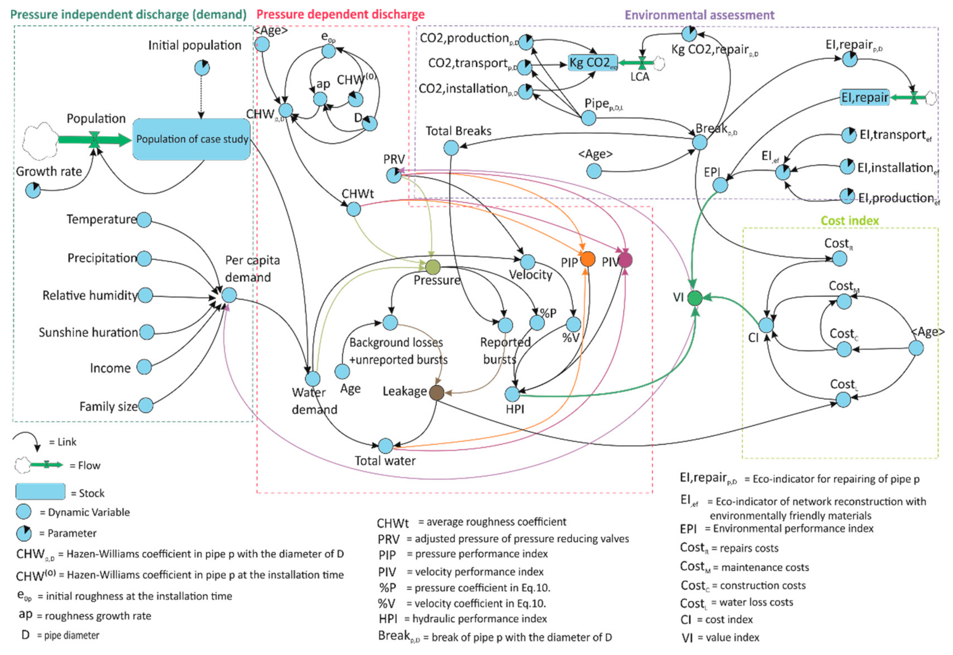
The framework of the developed SD model for WDNs is illustrated in Figure 2. AnyLogic7 software is used to simulate the feedbacks and interactions between the variables. According to Figure 2, this framework consists of different parts, including: pressure independent discharge (demand), pressure-dependent discharge, environmental assessment, and CI model. Some of the empirical equations, which are considered in the models, are shown in Table 1. In the demand model, the pressure independent discharge (demand) is calculated considering the climate, economic, and social variables. To develop a relationship between demand and these variables, the pressure independent discharge is calculated regarding the total inflow data and estimated leakage (Section 2.2.1). For this purpose, according to Equation (6), the emitter coefficient (C) is obtained and then is put in EPANET. On the other hand, if the total inflow is available, it is possible to compare the summation of leakage and demand of all nodes which are calculated in the hydraulic model, with the total inflow data. Using this method, the pressure independent discharge (demand) and the pressure-dependent discharge (leakage) are obtained in each time step. Then, employing the monthly demand, a relationship is introduced to calculate the per capita demand based on the different variables in the SD model. Another part of the SD framework is the pressure-dependent discharge model. In this model, the average pressure of nodes and average flow velocity in pipes are simulated. The average pressure and flow velocity are the functions of the following variables:
- Pipe roughness coefficient: hydraulic capacity of pipes decreases over time. In general, reducing hydraulic capacity is the result of increasing roughness in pipes. As roughness of a pipe increases, roughness coefficient decreases. Thus, according to the Hazen–Williams Equation (14), overall head loss increases and pressure decreases as a result. Therefore, the pipes’ roughness coefficients are directly related to the pressure of WDNs. In the SD model, Equation (15) is used to consider the changes in Hazen–Williams coefficient in each pipe [44]. Average roughness coefficient of a network (CHWt) as the representative of the whole system roughness is calculated by weighting the coefficient of each diameter based on its length.
- Demand changes: The pressure independent discharge (demand) is the second variable on which the pressure and velocity of WDNs are dependent. Increasing the demand results in increasing the consumption which reduces the pressure of the nodes and increases the flow velocity in the pipes.
- Adjusted pressure of pressure-reducing valves (PRV): adjusted pressure of PRV valves can have a significant effect on the pressure and velocity of the system.
After determining the average pressure, the real loss is estimated. Real loss in WDNs is categorized into reported bursts, unreported bursts, and background losses. Although reported bursts have a large amount of discharge, due to the low frequency and short duration of them, they usually make a small part of the total leakage in comparison with unreported bursts and background losses. On the other hand, the accurate measurement of unreported bursts and background losses is not possible because of economic or technical constraints [35]. Based on the proposed model and using standard codes, when the accurate real loss data is not recorded, leakage in the SD model is classified into two parts:
- Discharge of the background losses and unreported bursts: it is considered as the function of the average pressure and average age of the system (Equation (18)).
- Discharge of the reported bursts: regarding the guidelines [41], it is considered as the function of total breaks, the flow rate of burst, the average pressure of the system, and the duration of the total breaks (Equation (19)). The break rate of the pipes is calculated based on Equations (20) and (21) [45]. According to the previous studies and guidelines [41,46], the flow rate of burst () is considered 12 . The parameters of A, B, C in Equation (18) and t (the total break duration) in Equation (19) are determined by calibration of these equations with the leakage calculated based on MNF method. For this purpose, OptQuest calibration module [47,48] in AnyLogic software is used. This module minimizes the difference between the simulated and observed leakage. This process is basically an optimization process which its objective function is defined in accordance with Equation (22).
By calculating leakage, the total water flow to the network in each SD time step is equal to the sum of the leakage and water demand. To evaluate the hydraulic performance in the SD model, PIP and PIV are defined based on the total water flow, total roughness coefficient, and the set pressure of PRV valves. Then, to calculate HPI (Equation (10)), the variables of
α, β, γ, and δ are determined by analyzing the network for different values of average pressure and velocity.
Next part of the SD model is the environmental assessment, in which the environmental impacts of WDNs are evaluated. In this model, according to the number of breaks for each diameter and the LCA functional unit in the operation phase, the cumulative in each time step is determined. Besides, for evaluating the environmental impacts of the operation phase, EPI is calculated in the SD model based on Equation (1). Finally, the accuracy of the SD model is evaluated in order to investigate the correlation between the simulated and observed data in the developed model based on the coefficient of determination, Root Mean Squared Error (RMSE), and the ratio of observed and simulated standard deviation. A description of these indices can be found in the Supplementary Materials.
3. Case Study
To illustrate the applicability of the proposed method, a part of Tehran’s WDN, which supplies water for 114,849 inhabitants in an area of about 413 hectares, is selected as the study area. The total length of the pipeline in the considered WDN is about 77 km with an average age of 26 years. The pipe materials installed in the WDN are ductile iron (with the diameters of 150, 200, 250, 400, 500 mm) and steel (with the diameter of 600 mm). In addition, high-density polyethylene (HDPE) pipes have been used for renovating some parts of the system since 2018. The per capita water consumption was reported about 240.7 LPCD (liters per capita per day) in 2015. Data of inflow to the network is available from 2012 to 2016 [31]. Using this data, the performance of the WDN is simulated in the monthly time steps from 2007 to 2016. This case study is comprised of six pressure zone. The characteristics of these pressure zones and schematic of the WDN are shown in the Supplementary Materials (Table S3, Figure S2). There are six valves in this network, which are currently adjusted on the pressure of 30 m. During evaluating the performance, the pressure of these valves remains constant. However, in the performance enhancement scenarios, the effects of changing the pressure of these valves on the system are investigated. According to the defined SD framework (Figure 2), some of the regression equations developed based on the case study data are indicated in Table 1. For instance, considering different climate and socioeconomic variables [49], the per capita demand is simulated according to Equation (23), using the multivariate linear regression model. In addition, in each SD time step, the average pressure and velocity of the network are calculated using Equations (24) and (25). After evaluating the performance of the network in the SD framework, scenarios are applied to improve the value index of the WDN. For this purpose, four scenarios are considered as follows: (1) reducing the per capita water demand; (2) decreasing the average pressure; (3) reducing the age of the system by its pipes renewing; and, (4) a combination of reducing the per capita water demand and reducing the average pressure in the WDN. These scenarios are proposed based on TPWWC’s plans. For instance, since 2014, per capita water demand reduction program has been applied to this WDN. Moreover, due to the high break rate of the pipes, a part of the WDN has been taken in the priority of replacement. Additionally, pressure management is another plan to control the leakage and improve the performance of the network.
4. Results and Discussion
4.1. Environmental Impacts Assessment
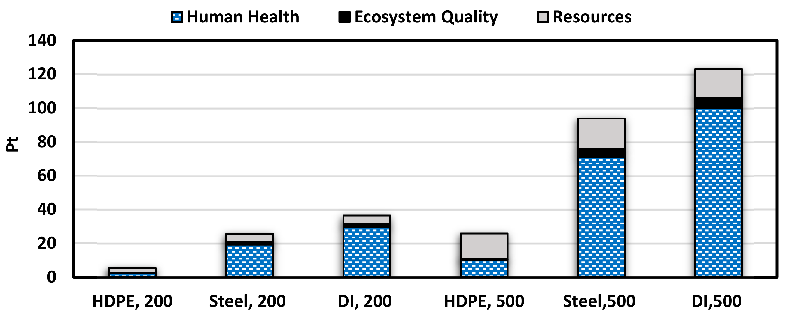
To compare the environmental impacts of different pipes, diameters of 200 and 500 mm are chosen as the representative of the other diameters. Figure 3 illustrates a comparison of the endpoint impacts of different pipes in the total phases of production, transportation, and installation based on the defined functional unit. Figure 3 indicates that HDPE pipes have the least environmental impacts, while ductile iron and steel are the most environmental impacting pipes. One of the main reasons is that more raw materials used in the manufacturing process of ductile iron and steel pipes, compared to other pipes. For instance, 36 kg of materials (including cast iron, cement mortar, bitumen, and zinc oxide) are required for manufacturing one meter of the ductile iron pipe with 200 mm diameter, while needed materials for manufacturing the HDPE pipe with the same length and diameter are 8.5 kg. Since HDPE pipes have the minimum impacts, the term of in the Equation (1) is allocated to the HDPE pipes.
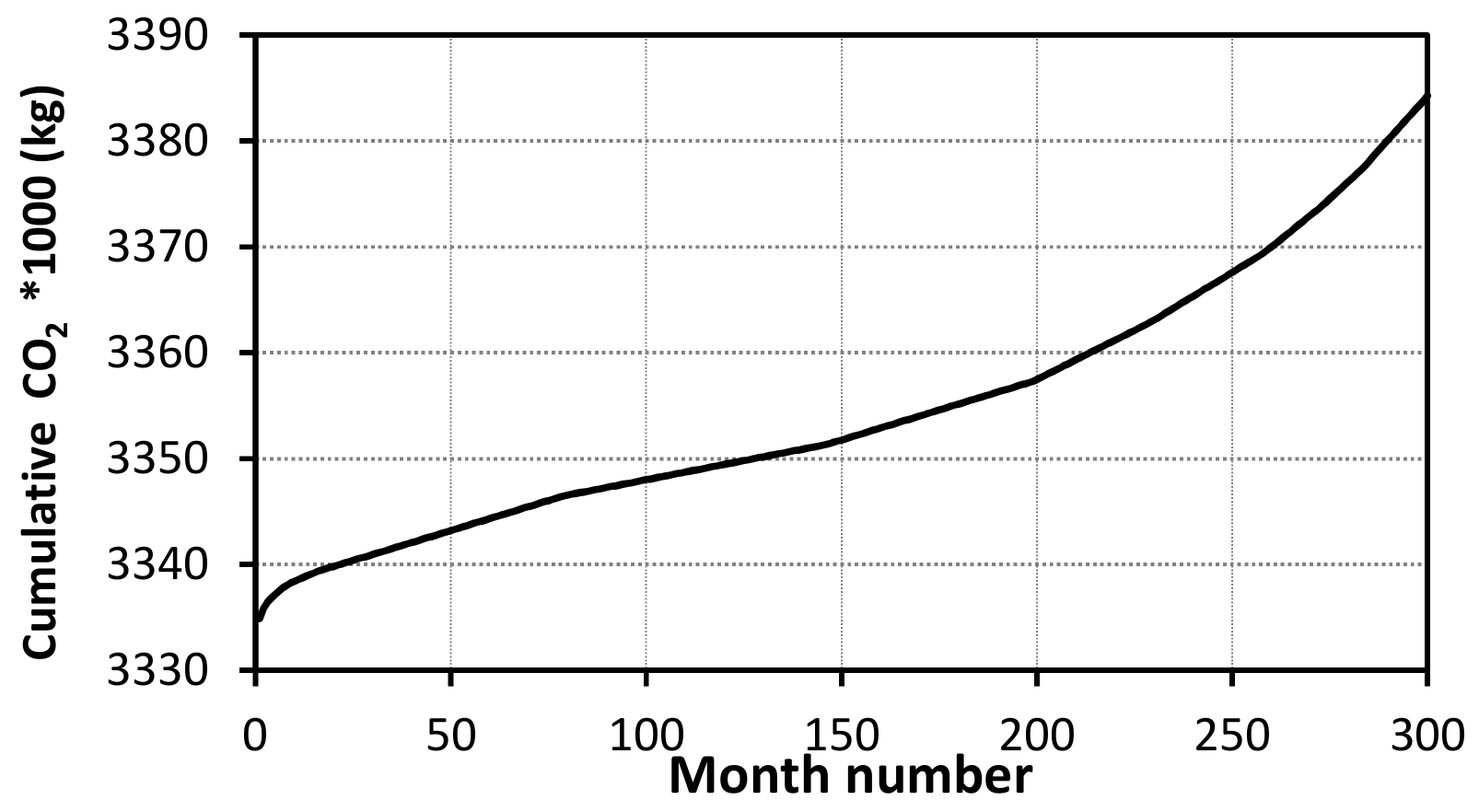
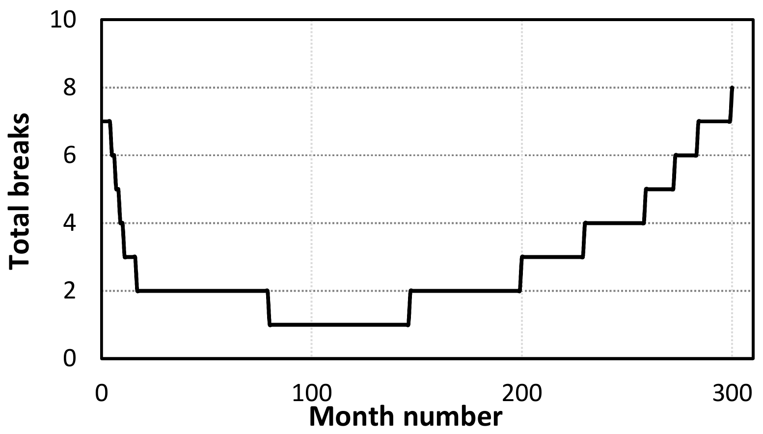
To analyze the environmental impacts during the operation time, the cumulative is assessed in the SD model. Figure 4 illustrates the amount of released cumulative during the construction time (1992) until the end of simulation time with the monthly time steps. In addition, the total number of pipes breaks in each month are shown in Figure 5. In the early months of operating, the failure rate of the pipes is high, so the environmental impacts of the WDN are increased according to Figure 4. On the other hand, as shown in Figure 5, in the middle months, the number of total breaks is reduced and becomes almost constant, thus, there is a steady rise in the cumulative release until month 200 (Figure 4). From month 200 until 300, due to pipes aging, there is a sharp increase in the cumulative release. In WDNs with pumping stations, the main environmental impacts in the operation phase are due to energy consumed for pumping water [50]. Therefore, if there is a pump in the system then a reduction in water consumption could reduce the environmental impact compared to previous time steps. In this paper, since the proposed environmental index is applied for a WDN without pumps, the environmental effects of the operation phase are mainly due to pipes breaks. On the other hand, if less capacity is required in the future, then smaller diameters are needed for redesigning networks, which leads to some positive effects on environmental impacts. However, in this study, in order to develop the model in a simple way, the redesign process of WDNs in the operation phase is not considered. In other words, it is assumed that the system has the same capacity during the operation phase. In this case study, approximately 800 kg of equivalent is released during the 8th year of operation (from 96 until 107 months), while it is raised to around 4100 kg/year in the last year of simulation time (2015–2016).
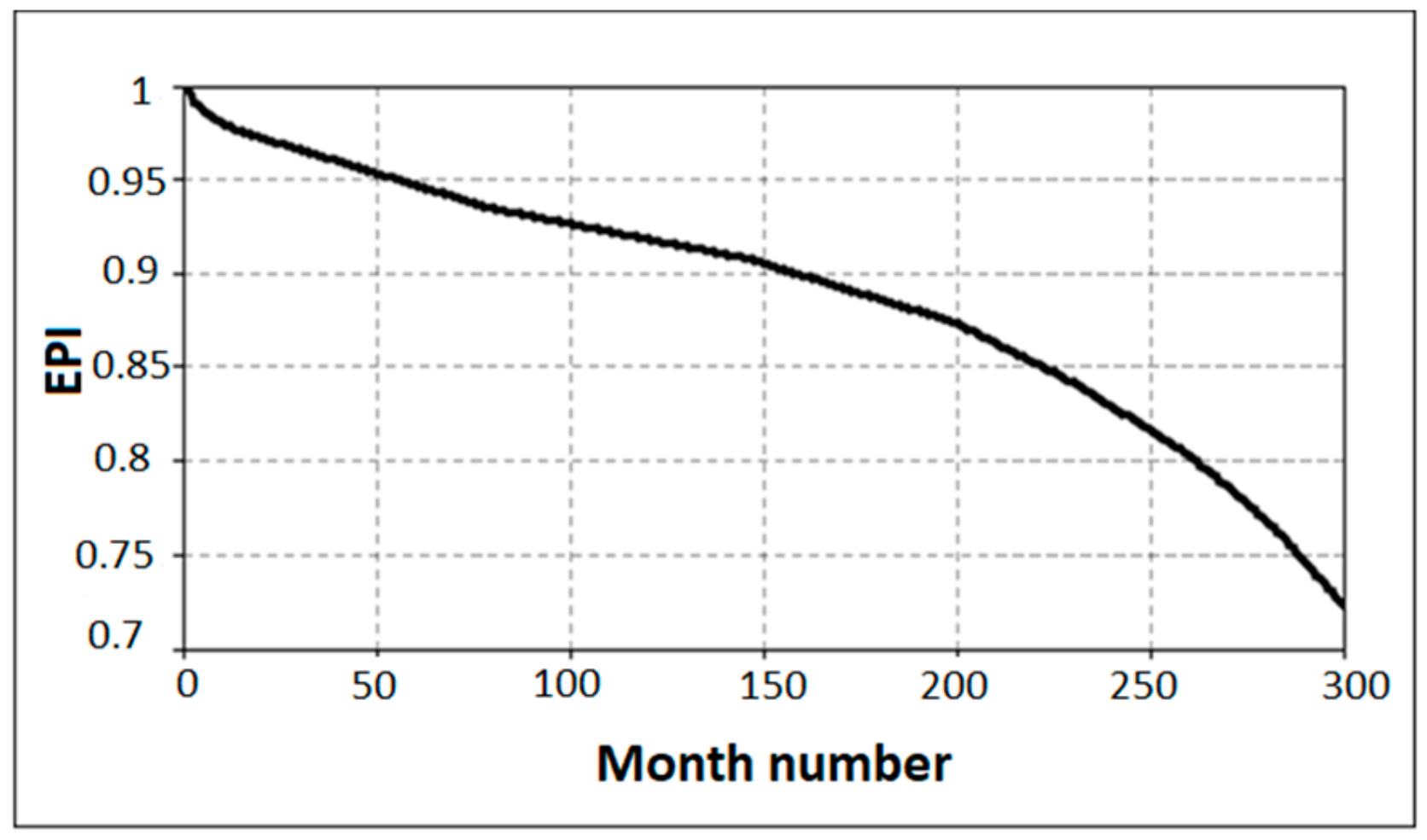
Figure 6, shows changes of EPI since the construction of the network. As illustrated, from month 200, there is a significant drop in EPI compared to the previous months. The reason is that the failure rate of the pipes, from this time step, is raised, which increases the environmental impact of the operation phase and, consequently, decreases EPI. At the end of the modeling time, EPI is higher than 0.7. Since the values of 0.75, 0.5, and 0.25 describe the suitable, acceptable, and unacceptable performance level of the system, respectively, it can be concluded that EPI is in the suitable level in most of the operation time.
4.2. Calibration of the Leakage Equation
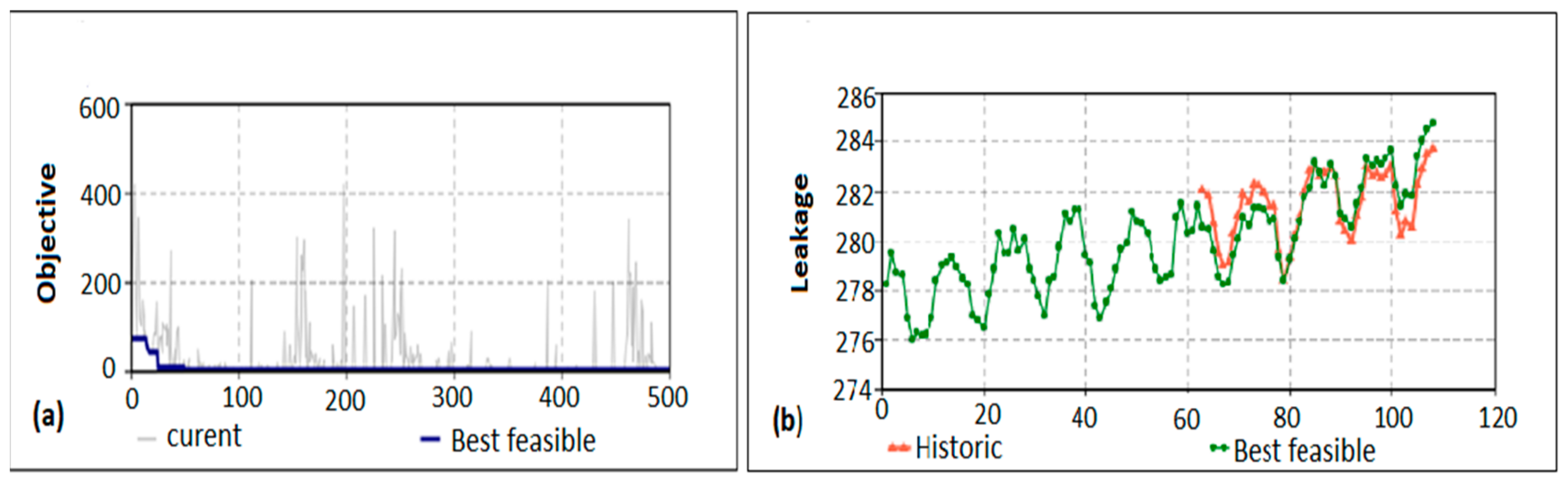
Using OptQuest calibration module in AnyLogic software, parameters of A, B, and C in Equation (18) and t in Equation (19) are calibrated with the leakage calculated based on MNF method from 2012 to 2015. Figure 7a indicates changes of the objective function value (current) at any iteration (Equation (22)), and the optimal value of the objective function until each iteration (best feasible). Moreover, the values of the observed and simulated leakage during the optimization process are demonstrated in Figure 7b. According to Figure 7a, there is a major difference between the observed and simulated leakage until the 20th iteration. However, from the 20th iteration, this difference decreases and the optimal value of the objective function is improved compared to the previous repetitions. Consequently, the convergence process of the objective function is started since the 20th iteration. Since the termination condition is 500 times iterations without improvement in the optimal objective function, the optimization process is stopped at the end of 500 repetitions. The results of the calibration process are presented in Table 2.
4.3. Correlation between the Simulated and Observed Inflow
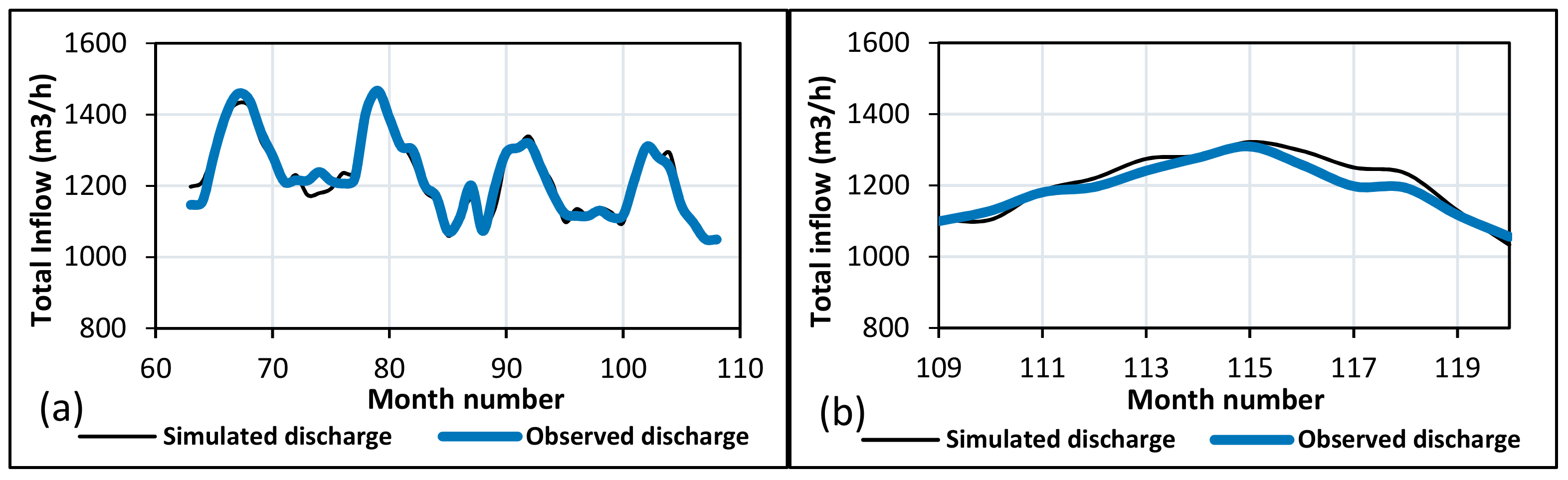
After modeling the pressure-dependent discharge (Leakage) in the SD model, the mean inflow to the network is equal to the sum of the leakage and pressure independent discharge (demand). Available inflow data from 2012 to 2015 are used for calibrating the model. Moreover, inflow data of 2016 is employed for the model validation. Figure 8a indicates the simulated and observed discharge after calibrating the leakage coefficients. Moreover, the total inflow in the validation phase is shown in Figure 8b. According to Table 3, since the values of coefficient of determination (R), and ratio of observed and simulated standard deviation (RS) (see Supplementary Materials) are greater than 0.9, there is a good correlation between the simulated and observed data. Additionally, the value of RMSE after calibration is 24.4 . As the mean inflow is around 1200 , the ratio of RMSE to average discharge is about 2%, which is an acceptable value.
4.4. Evaluation of the Leakage, Pressure, and Inflow of the WDN
Figure 9a demonstrated the simulated leakage of the WDN. Moreover, the values of total inflow and average pressure are indicated in Figure 9b,c. As shown in Figure 9a, there is an increase in the annual simulated leakage over time. The age of the system is increasing which leads to a gradual rise in the leakage according to Equation (18). On the other hand, Figure 9b indicates that total inflow to the WDN is decreased in the demanding months since the 84th month (from 2014), which consequently increases the average pressure in these time steps (Figure 9c). Therefore, as demonstrated in Figure 9a, increasing the average pressure of the system has a significant effect on the leakage since the 84th month (from 2014). Reducing the total inflow is due to the per capita demand reduction in the study area which has been done by TPWWC since 2014.
4.5. Evaluation of the Leakage, Pressure, and Inflow of the WDN
HPI is calculated based on the penalty curves (Figure 1), the percentage of pressure less than 30 m and greater than 50 m , and the percentage of the pipes with the flow velocity less than 0.8 m/s and greater than 2.5 m/s . Changes of these variables in each SD time step are shown in the Supplementary Materials (Figure S3). Figure 10 indicates HPI of the WDN during the simulation time. This figure illustrates that regarding the excess pressure in the network, in months, like month 80, in which the inflow to the WDN is high (Figure 9b) and consequently, pressure is lower (Figure 9c) and velocity is higher than other time steps, HPI is improved. On the other hand, reducing the total inflow to the WDN since the 84th time step, in the demanding month like 102, increases the average pressure, decreases the velocity of pipes, and finally leading to declining HPI.
4.6. Evaluating VI of the System
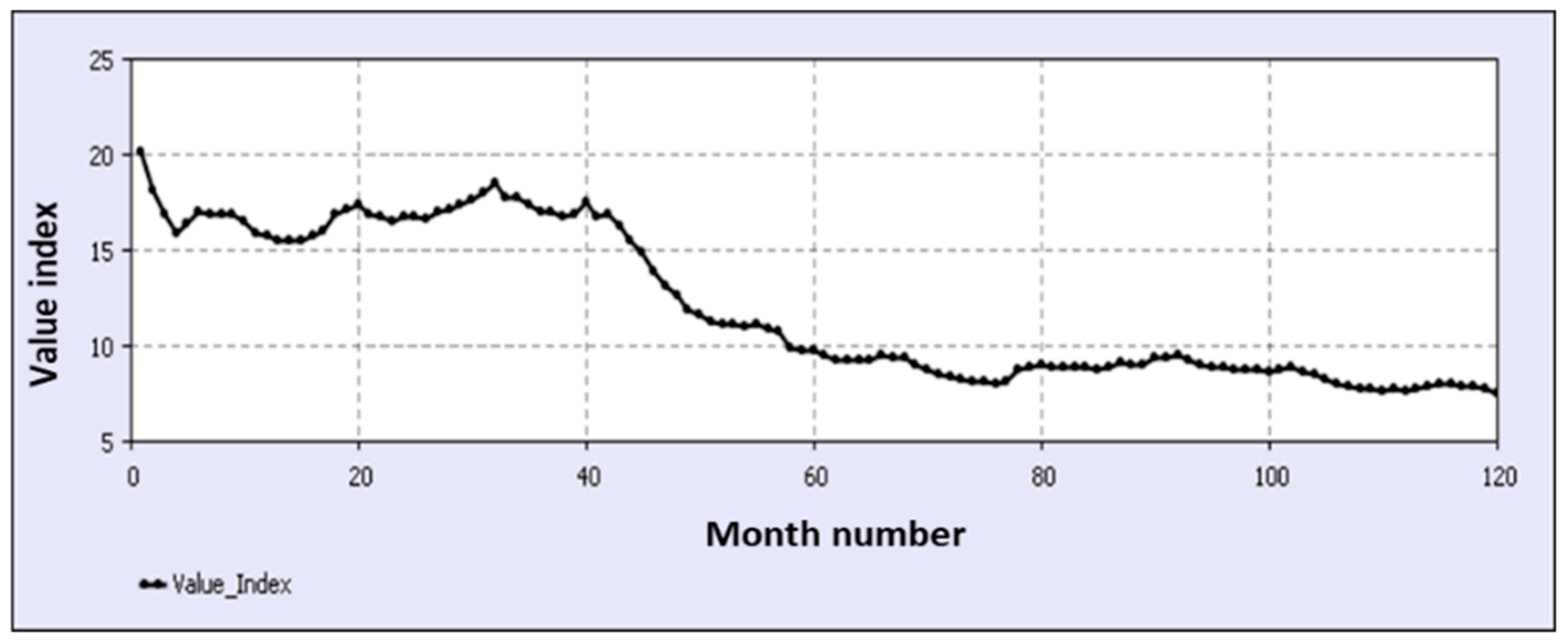
The changes of VI are illustrated in Figure 11. Accordingly, from the 5th to 40th month, the trend of changes of VI is almost ascending in each year. Between the 41st and 76th months, the operation costs of the WDN (costs of maintenance, repairs, and water losses) are increased to more than the reconstruction costs. Therefore, it causes an increase in CI and, subsequently, decreases VI. From month 84 until month 120, as the reconstruction costs increase rapidly, CI decreases. Moreover, due to the excess pressure and aging of pipes, the performance of the WDN is declined. Thus, in this time period, VI remains constant.
4.7. Scenarios for Improvement of VI
As shown in Figure 11, before the 46th time step of system operation, VI is always more than 15 but after this month, it shows a descending trend. However, from the beginning of the 60th month to the end of the modeling time period, VI changes show a steady behavior. Consequently, the enhancement scenarios are considered for the time steps 46–120, which VI is less than 15.
4.7.1. Scenario 1: Reducing the Per Capita Water Demand
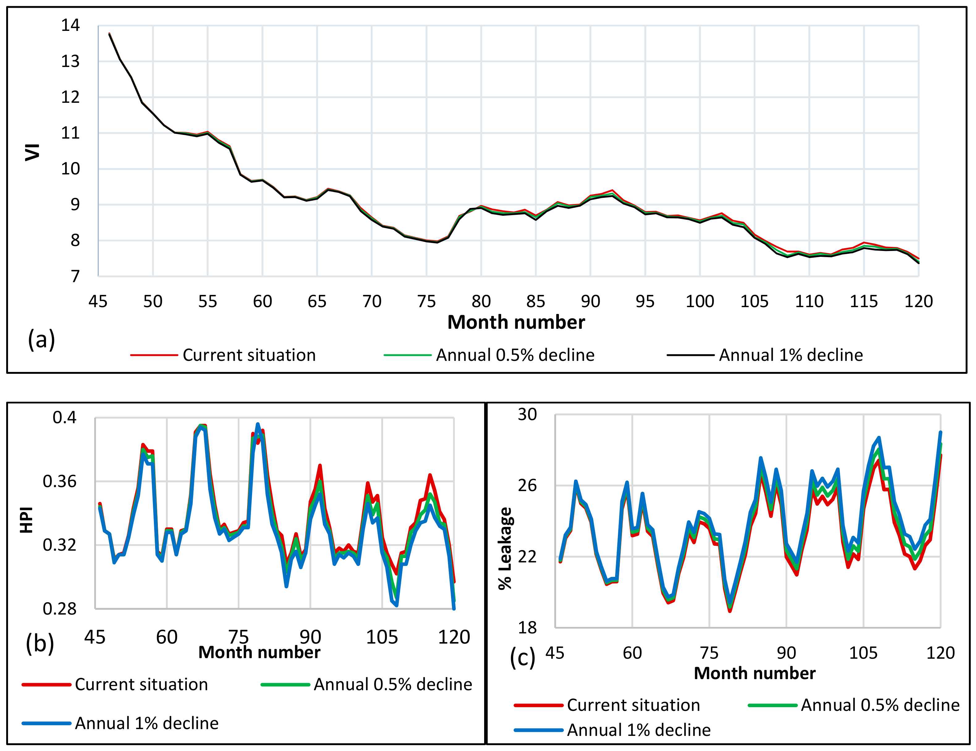
In this scenario, the effects of reducing the per capita water demand program are investigated over time. Since the results of per capita water demand reduction program are gradually observed, the annual reduction of 0.5% and 1% in the per capita water demand is applied from 46th to 120th time steps (during 6 years), in the SD model. As indicated in Figure 12a, in the early months, the annual decline in the per capita water demand does not have a significant effect on VI. However, at the end of the simulation period, it leads to a slight decline in VI. For example, in the final step, the value of VI without applying water demand reduction is 7.49, whereas this amount is 7.41 and 7.37, respectively, when the per capita water demand is reduced by the annual rate of 0.5% and 1%.
As mentioned before, there is surplus pressure in the system. Moreover, flow velocity in most of the pipes is less than the optimum value. Reducing the per capita water demand increases the average pressure of the system and decreases the total inflow. Consequently, as the rate of per capita water demand reduction is increased, HPI is decreased (Figure 12b). On the other hand, because of the increase in the average pressure of WDN, the leakage is raised (Figure 12c) and the water losses costs are increased subsequently. Therefore, VI is reduced during the simulation time. Figure 12c shows that the mean leakage without application of water demand reduction program is 23.2%, whereas, in the annual reduction of 0.5% and 1% of per capita water demand, this amount is 23.6% and 24%, respectively.
4.7.2. Scenario 2: Reducing the Average Pressure
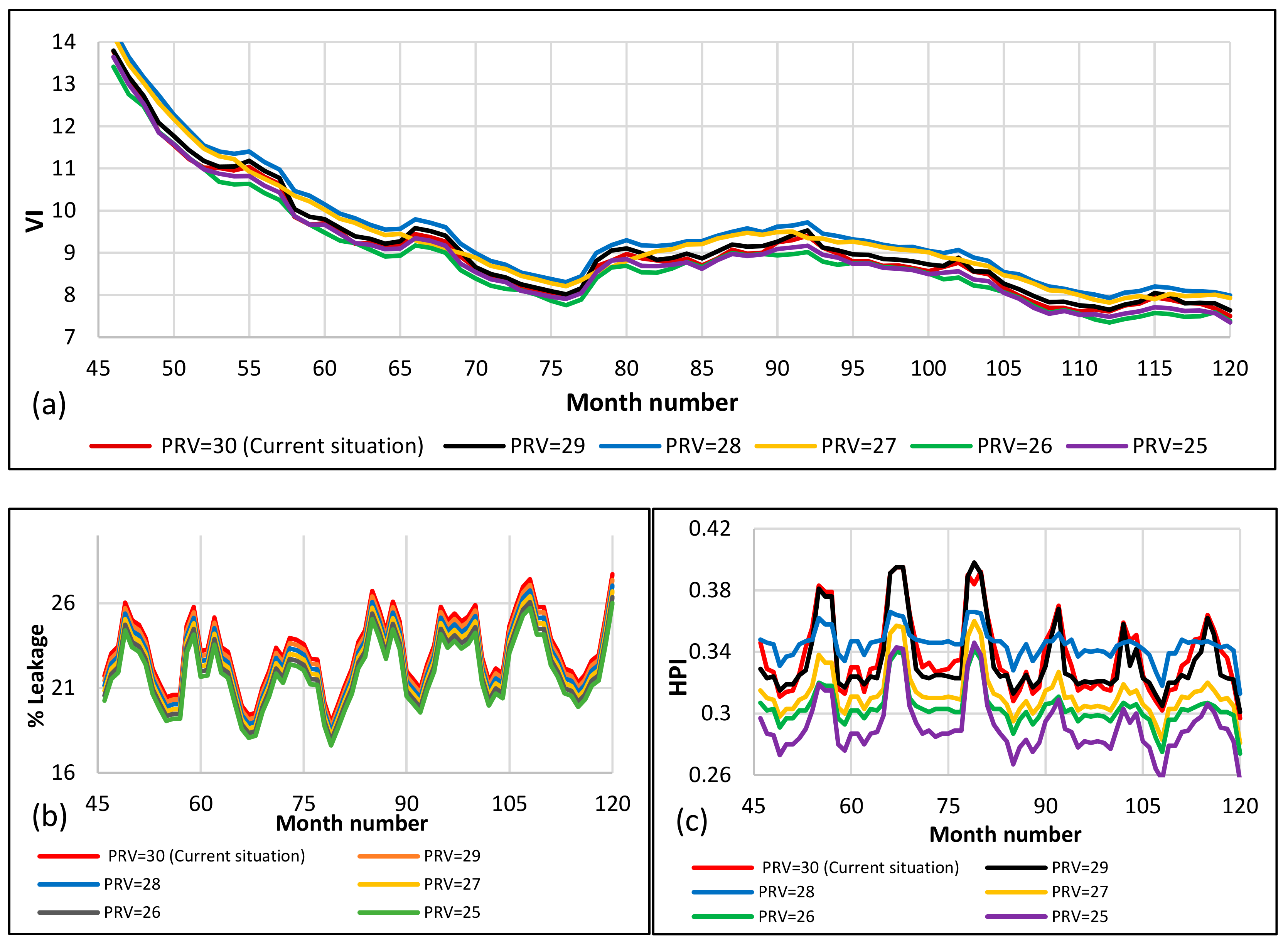
The WDN has six PRV valves that are currently adjusted on the pressure of 30 m. In the current situation, the average pressure of the WDN changes in a range of 37.2 m to 38.3 m (Figure 9c). Considering the value of 30 m as the desired pressure, it can be concluded that there is about 7–8 m excess pressure in the WDN. Therefore, in this scenario, the average pressure of the WDN is decreased by reducing the adjusted pressure of the PRV valves, which is applied from the 46th month and remains constant until the end of the modeling period. As illustrated in Figure 13b, by reducing the average pressure of WDN, the leakage of the system decreases and, consequently, the water loss costs and CI are decreased. Figure 13a indicates that when the pressure of the PRVs are adjusted on 28 m (PRV = 28 m), VI is greater than PRVs = 29 and PRVs = 30. When the PRVs pressure is set on 30 m, the pressure in 9%–15% nodes is greater than 50 m () and the pressure is less than 30 m in about 19% of the nodes ( (Figure S3). However, when the PRVs pressure is set on 28 m, the average pressure of WDN changes in a range of 35.6 m to 36 m in most of the time steps, in which the values of and are 2.5 and 25, respectively. Thus, the pressure reduction of the PRV valves to 28 m reduces the average pressure of the WDN, increases HPI in most of the time steps (Figure 13c), reduces CI in all months (due to the water losses costs reduction), and, finally, increases VI.
Figure 13a shows that by decreasing the adjusted pressures of PRVs until 25 m, VI is reduced compared with when the PRVs are set on 27 m. The reason is that, by reducing the PRVs pressure until 25 m, the percentage of the nodes with the pressure greater than 50 m remains constant (2%), while the percentage of the nodes with the pressure less than 30 m is increased. For instance, when the PRVs are set on 25 m, the average pressures in most of the months changes in a range of 32.5 m to 33 m and the values of and are 2 and 42, respectively. Therefore, in this scenario, the best VI is allocated to the situation in which the PRV valves are adjusted on 28 m.
4.7.3. Scenario 3: Reducing the Age of the System by Renewing Pipe
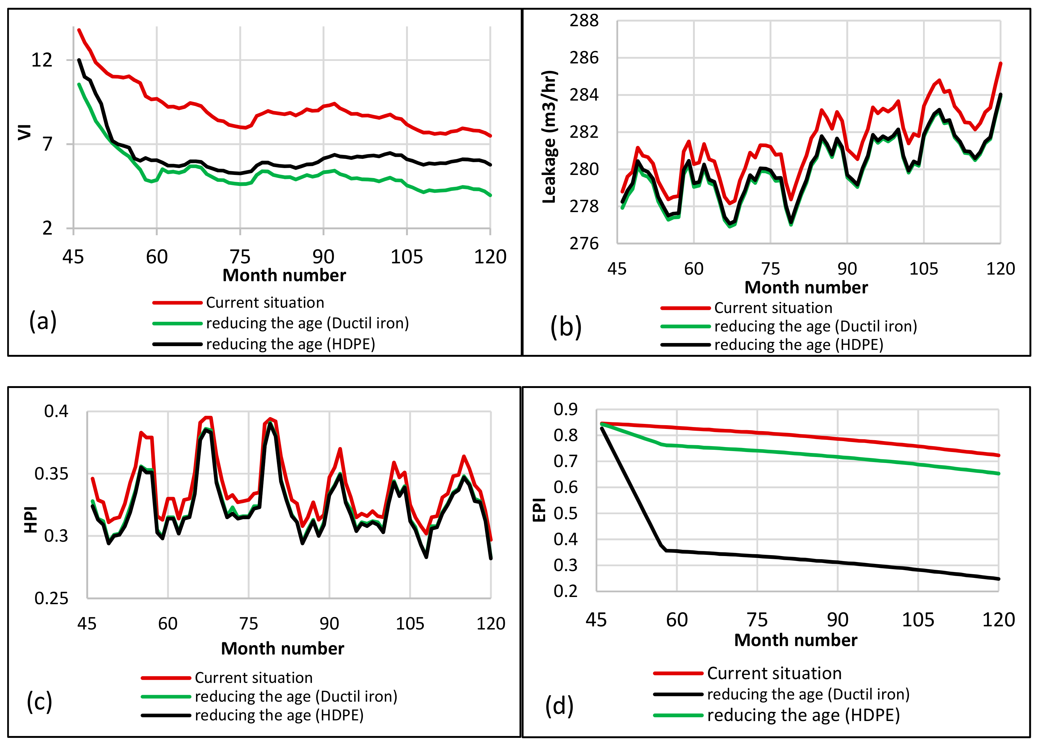
Because of the usage of HDPE (200 mm) pipes for renewing the WDN [31], the effects of replacement of the old ductile iron pipes (200 mm) with new HDPE and ductile iron pipes are investigated in this scenario. It is assumed that the pipes with the diameter of 200 mm are replaced from the 46th month for 12 months. The length of 200 mm pipes is about 3 km, therefore, 250 m of old pipes are substituted with the new pipes in each month.
In this scenario, the average age of the system is reduced four years in the final step. Hence, according to Equation (18), the leakage is decreased. On the other hand, by substituting the new pipes, the average roughness coefficient (CHWt) of the WDN is increased, which causes a slight increase in the average pressure. Nevertheless, this increase is negligible in the average pressure and, consequently, the leakage is decreased due to fewer breaks of pipes (Figure 14b). The Hazen–Williams coefficient of HDPE pipes is higher than ductile iron pipes. Therefore, as demonstrated in Figure 14b, the leakage reduction in renewing the network with the HDPE pipes is less than when the ductile iron pipes are used for renewing. According to Figure 14c, increasing the average pressure causes a reduction in HPI. Moreover, Figure 14d shows that EPI is declined because of the environmental impacts of WDN reconstruction. Finally, as illustrated in Figure 14a, renewing the network with ductile iron or HDPE pipes does not have an effective role in improving VI.
4.7.4. Scenario 4: Reducing the Per Capita Water Demand and Average Pressure
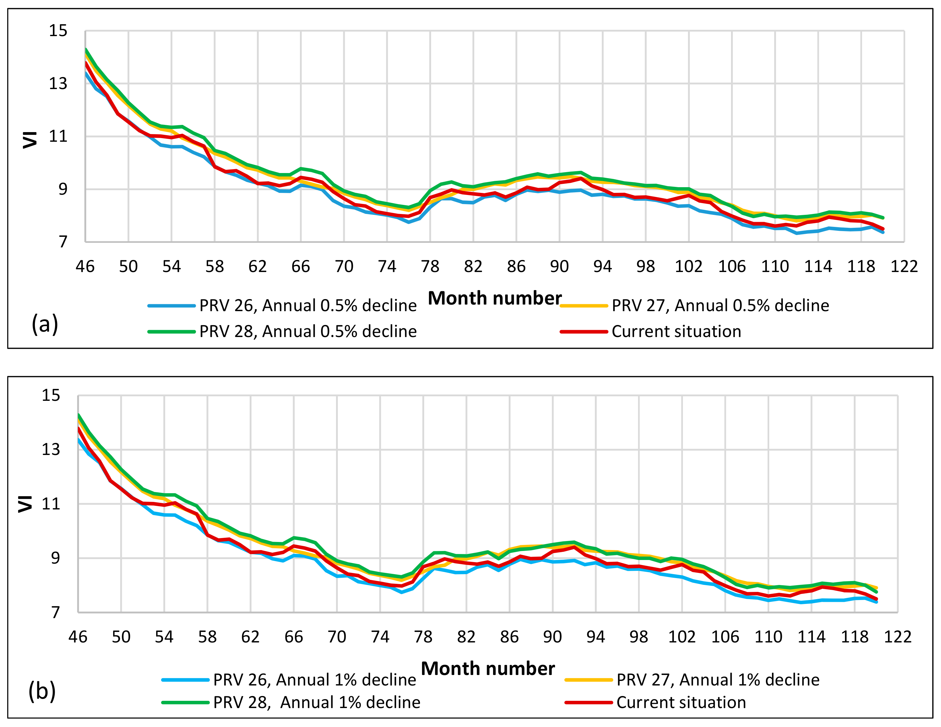
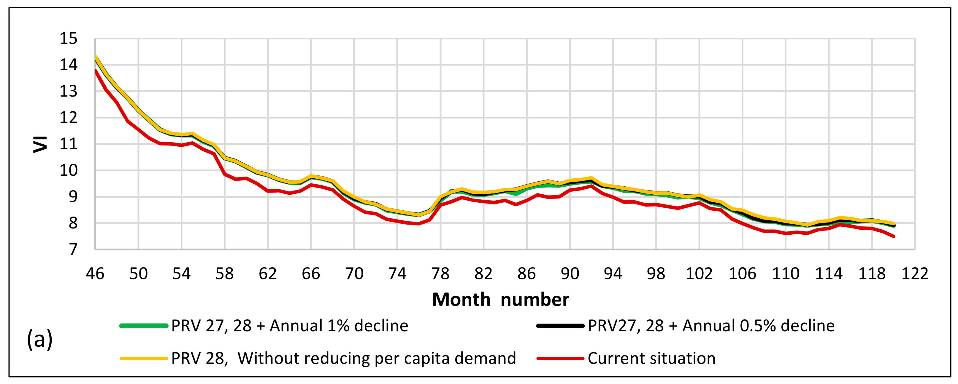
In this scenario, VI changes are examined by reducing the pressure of the PRV valves as well as annual per capita water demand simultaneously. For this purpose, the performance of the WDN is investigated in an annual reduction of 0.5% and 1% of per capita water demand, in which the PRVs are set on the pressure of 28 m, 27 m, and 26 m. According to Figure 15a, up to the time step of 105, the adjusted pressure of 28 m for PRVs has the highest VI in the annual reduction of 0.5% of the per capita water demand. In fact, the reduction of PRVs setting from 30 m (current situation) to 28 m declines the excess pressure, increases HPI, decreases the costs of water losses, and, thus, increases VI. However, from the time steps of 106–110, the adjusted pressure of 27 m has the highest VI. The reason is that the average pressure of the WDN has the highest value in the range of time steps 106–110 (Figure 9c). From the time steps of 111–120, the best VI is achieved when the PRV setting is equal to 28 m. Increasing the rate of per capita water demand reduction from 0.5 to 1% lead to an increase in the number of time steps in which PRVs = 27 m have the maximum values of VI. As demonstrated in Figure 15b, the highest values of VI in the annual reduction rate of 1% are in the time steps of 85–88, 95–100, 106–110, and 119–120, in which the PRV valves are adjusted on 27 m. In other months, the highest values of VI are observed when the PRVs setting is equal to 28 m.
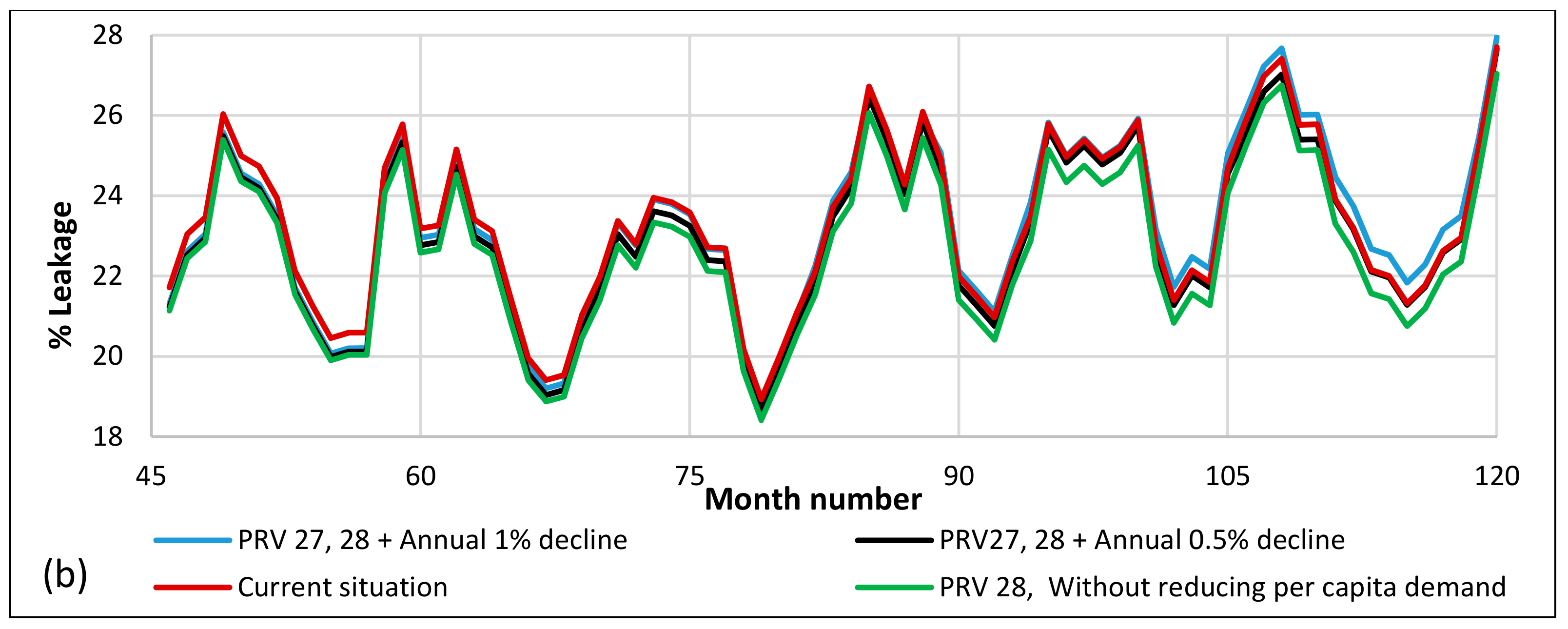
4.7.5. Comparing the Best Scenarios
Comparing the best values of VI in the 2nd and 4th scenarios in Figure 16a, it can be concluded that the effective scenarios in improving VI are very similar. In general, it can be seen that the reduction of PRVs pressure setting to 28 m without reducing the per capita water demand (2nd scenario) has the best effect on enhancing VI in the WDN. Figure 16b demonstrated the percentage of leakage in the scenarios, which have the best VI. The mean leakage in the current situation is 23.2%, whereas, in the annual reduction of 0.5% and 1% of per capita water demand with decreasing the pressure setting of PRV valves, this amount is 23% and 23.2%, respectively. Additionally, the mean leakage is 22.7% in reducing the pressure setting of PRV valves to 28 m (2nd scenario).
5. Summary and Conclusions
In this paper, using SD approach, an algorithm is proposed in order to improve the performance of WDNs. For this purpose, with regard to the hydraulic variables (pressure and velocity) and environmental impacts of WDNs, new hydraulic and environmental indicators are developed. Moreover, CI is presented to evaluate the operation costs of the networks in each SD time step. Then, the performance of the network is assessed based on the VI which evaluates the hydraulic and environmental indices relative to the costs of WDNs. The environmental impacts analyses show that increasing age of pipes causes growth in the rate of failure and, consequently, increases the equivalent emissions of the operation phase from 800 kg in the 8th year to 4100 kg in the final time step. Furthermore, the pipe materials (especially ductile iron) have significant effects on the environmental impacts. The results of the hydraulic performance indicate that the surplus pressure causes large amounts of water loss during the operation time, so that the mean leakage is 23.2% in the case study. Changes in VI during the modeling time demonstrate a downward trend of VI beginning from the 46th time steps. Therefore, the improvement scenarios are considered for the months of 46–120, according to the requirements of the WDN. Based on investigating VI in each scenario, it can be concluded that reducing the per capita water demand and renovating some parts of the network do not have a significant role in performance enhancement. In contrast, the best solution for increasing VI is to reduce the pressure setting of PRV valves from 30 to 28 m. This scenario increases the performance, declines operation costs, and, consequently, increases the average value of VI from 9 to 9.5.
In WDNs some internal and external variables such as population, demand, pipe aging, and pressure affect the performance of the system. The proposed SD framework in this study is comprised of main variables of WDNs which allows managers to apply it for other case studies, considering their own indicators (e.g., resilience, reliability, redundancy). Supplementary to this, the proposed VI in the SD model can be useful for decision-makers to evaluate the performance and costs of WDNs during the operation phase. This is significant because some variables in WDNs like pipe aging not only affects the performance of the system but also cause an increase in the costs of the operation phase.
Supplementary Materials
The following are available online at https://www.mdpi.com/2073-4441/11/12/2445/s1, Table S1: Summary of items included and excluded in the system boundaries, Table S2: Inventory data for 200 mm Ductile Iron (DI) pipe based on the functional units of different phases, Table S3: The characteristics of each pressure zone in the considered WDN, Figure S1: Dimensions of the considered trenches in the installation phase, Figure S2: Schematic of the WDN, Figure S3: Changes of the variables used in Hydraulic Performance Index (HPI) calculation during the simulation time (2007–2016): (a) & ; (b)
Author Contributions
M.H. designed the framework, performed the analysis, and wrote the draft; S.N. supervised the research, helped in developing the model, and edited the writing; R.S. helped in improving the model and editing the manuscript.
Funding
This research was funded by the Austrian Science Fund (FWF): P 31104-N29.
Acknowledgments
The authors gratefully acknowledge Tehran Province Water and Wastewater Company for providing the required data. “Open Access Funding by the Austrian Science Fund (FWF).”
Conflicts of Interest
The authors declare no conflict of interest.
References
- United Nations Educational Scientific and Cultural Organization (UNESCO). The United Nations World Water Development Report 4: Managing Water Under Uncertainty and Risk; United Nations Educational Scientific and Cultural Organization (UNESCO): Paris, France, 2012; Volume 1. [Google Scholar]
- Veldkamp, T.I.E.; Wada, Y.; Aerts, J.; Döll, P.; Gosling, S.N.; Liu, J.; Masaki, Y.; Oki, T.; Ostberg, S.; Pokhrel, Y. Water scarcity hotspots travel downstream due to human interventions in the 20th and 21st century. Nat. Commun. 2017, 8, 15697. [Google Scholar] [CrossRef] [PubMed]
- Grigg, N.S. Main Break Prediction, Prevention, and Control; American Water Works Association: Denver, CO, USA, 2007; Volume 75. [Google Scholar]
- Sterman, J.D. System dynamics modeling: Tools for learning in a complex world. Calif. Manag. Rev. 2001, 43, 8–25. [Google Scholar] [CrossRef]
- Zarghami, M.; Akbariyeh, S. System dynamics modeling for complex urban water systems: Application to the city of Tabriz, Iran. Resour. Conserv. Recycl. 2012, 60, 99–106. [Google Scholar] [CrossRef]
- Ahmad, S.; Simonovic, S.P. Spatial system dynamics: New approach for simulation of water resources systems. J. Comput. Civ. Eng. 2004, 18, 331–340. [Google Scholar] [CrossRef]
- Ahmad, S.; Simonovic, S.P. An intelligent decision support system for management of floods. Water Resour. Manag. 2006, 20, 391–410. [Google Scholar] [CrossRef]
- Madani, K.; Mariño, M.A. System dynamics analysis for managing Iran’s Zayandeh-Rud river basin. Water Resour. Manag. 2009, 23, 2163–2187. [Google Scholar] [CrossRef]
- Rusuli, Y.; Li, L.; Ahmad, S.; Zhao, X. Dynamics model to simulate water and salt balance of Bosten Lake in Xinjiang, China. Environ. Earth Sci. 2015, 74, 2499–2510. [Google Scholar] [CrossRef]
- Sharawat, I.; Dahiya, R.; Dahiya, R.P.; Sreekrishnan, T.R.; Kumari, S. Policy options for managing the water resources in rapidly expanding cities: A system dynamics approach. Sustain. Water Resour. Manag. 2019, 5, 1201–1215. [Google Scholar] [CrossRef]
- Sun, B.; Yang, X. Simulation of water resources carrying capacity in Xiong’an New Area based on system dynamics model. Water 2019, 11, 1085. [Google Scholar] [CrossRef]
- Qaiser, K.; Ahmad, S.; Johnson, W.; Batista, J.R. Evaluating water conservation and reuse policies using a dynamic water balance model. Environ. Manag. 2013, 51, 449–458. [Google Scholar] [CrossRef]
- Venkatesan, A.K.; Ahmad, S.; Johnson, W.; Batista, J.R. Systems dynamic model to forecast salinity load to the Colorado River due to urbanization within the Las Vegas Valley. Sci. Total Environ. 2011, 409, 2616–2625. [Google Scholar] [CrossRef] [PubMed]
- Neto, A.D.C.L.; Legey, L.F.L.; González-Araya, M.C.; Jablonski, S. A system dynamics model for the environmental management of the Sepetiba Bay watershed, Brazil. Environ. Manag. 2006, 38, 879–888. [Google Scholar] [CrossRef] [PubMed]
- Zhang, F.-Y.; Li, L.-H.; Ahmad, S.; Li, X.-M. Using path analysis to identify the influence of climatic factors on spring peak flow dominated by snowmelt in an alpine watershed. J. Mt. Sci. 2014, 11, 990–1000. [Google Scholar] [CrossRef]
- Simonovic, S.P.; Li, L. Methodology for assessment of climate change impacts on large-scale flood protection system. J. Water Resour. Plan. Manag. 2003, 129, 361–371. [Google Scholar] [CrossRef]
- Stojkovic, M.; Simonovic, S.P. System Dynamics Approach for Assessing the Behaviour of the Lim Reservoir System (Serbia) under Changing Climate Conditions. Water 2019, 11, 1620. [Google Scholar] [CrossRef]
- Salvitabar, A.; Zarghami, M.; Abrishamchi, A. System Dynamic Model in Tehran Urban Water Management. J. Water Wastewater 2006, 17, 12–28. [Google Scholar]
- Karamouz, M.; Goharian, E.; Nazif, S. Reliability assessment of the water supply systems under uncertain future extreme climate conditions. Earth Interact. 2013, 17, 1–27. [Google Scholar] [CrossRef]
- Dawadi, S.; Ahmad, S. Evaluating the impact of demand-side management on water resources under changing climatic conditions and increasing population. J. Environ. Manag. 2013, 114, 261–275. [Google Scholar] [CrossRef]
- Wu, G.; Li, L.; Ahmad, S.; Chen, X.; Pan, X. A dynamic model for vulnerability assessment of regional water resources in arid areas: A case study of Bayingolin, China. Water Resour. Manag. 2013, 27, 3085–3101. [Google Scholar] [CrossRef]
- Wei, T.; Lou, I.; Yang, Z.; Li, Y. A system dynamics urban water management model for Macau, China. J. Environ. Sci. 2016, 50, 117–126. [Google Scholar] [CrossRef]
- Chen, C.; Ahmad, S.; Kalra, A.; Xu, Z. A dynamic model for exploring water-resource management scenarios in an inland arid area: Shanshan County, Northwestern China. J. Mt. Sci. 2017, 14, 1039–1057. [Google Scholar] [CrossRef]
- Zarghami, S.A.; Gunawan, I.; Schultmann, F. System Dynamics Modelling Process in Water Sector: A Review of Research Literature. Syst. Res. Behav. Sci. 2018, 35, 776–790. [Google Scholar] [CrossRef]
- Karamouz, M.F.; Elyasi, A.; Ahmadi, A. An Algorithm for Evaluation of Water Resources Development. World Environ. Water Resour. Congr. 2008, 2008, 1–10. [Google Scholar]
- Li, C.; Liu, S.; Tao, T. Value engineering-based methodology of evaluating water distribution systems. Tongji Daxue Xuebao/J. Tongji Univ. Sci. 2006, 34, 646–650. [Google Scholar]
- Cuimei, L.; Suiqing, L. Water Distribution Systems Evaluating Method Based on Value Engineering: Case Study. In Water Distribution Systems Analysis Symposium 2006; American Society of Civil Engineers: Reston, VA, USA, 2008; pp. 1–11. [Google Scholar]
- Askarzadeh Farahani, M. Performance Evaluation of Water Distribution Networks Based on Value Engineering and Fuzzy Sets. Master’s Thesis, University of Tehran, Tehran, Iran, 2014. [Google Scholar]
- Li, C.; Li, S.; Wang, J.; Wang, H.; Zhang, S. The Comparison of the Value Engineering Method and Hydraulic Method on Water Distribution Systems Performance Evaluation. In World Environmental and Water Resources Congress 2011; American Society of Civil Engineers: Reston, VA, USA, 2011; pp. 4514–4522. [Google Scholar]
- International Organization for Standardization (ISO). ISO 14044—Environmental Management—Life Cycle Assessment—Requirements and Guidance; International Organization for Standardization: London, UK, 2006. [Google Scholar]
- Tehran Province Water and Wastewater Company (TPWWC). Statistics Obtained from the Director of Operation; Accessed on January 2017; Tehran Province Water and Wastewater Company (TPWWC): Tehran, Iran, 2017. [Google Scholar]
- Ecoinvent Swiss Centre for Life Cycle Inventories. Ecoinvent Database v3.0. Available online: http://www.ecoinvent.ch/ (accessed on 21 November 2019).
- Pre’ Consultants. SimaPro Database Manual; Pre’ Consultants: Amersfoort, The Nederlands, 2014. [Google Scholar]
- Roghani, B. Estimating the Sewerage Network Performance based on Value Engineering and Environmental Issues. Master’s Thesis, University of Tehran, Tehran, Iran, 2013. [Google Scholar]
- Tabesh, M.; Yekta, A.H.A.; Burrows, R. An integrated model to evaluate losses in water distribution systems. Water Resour. Manag. 2009, 23, 477–492. [Google Scholar] [CrossRef]
- Nazif, S.; Karamouz, M.; Tabesh, M.; Moridi, A. Pressure management model for urban water distribution networks. Water Resour. Manag. 2010, 24, 437–458. [Google Scholar] [CrossRef]
- Rossman, L.A. EPANET2 Users Manual National Risk Management Research Laboratory; US Environmental Protection Agency: Cincinnati, OH, USA, 2000.
- Lambert, A. Pressure Management/Leakage Relationships: Theory, Concepts and Practical Applications; IQPC Seminar: London, UK, 1997. [Google Scholar]
- Germanopoulos, G. A technical note on the inclusion of pressure dependent demand and leakage terms in water supply network models. Civ. Eng. Syst. 1985, 2, 171–179. [Google Scholar] [CrossRef]
- Tabesh, M.; Zia, A. Dynamic management of water distribution networks based on hydraulic performance analysis of the system. Water Sci. Technol. Water Supply 2003, 3, 95–102. [Google Scholar] [CrossRef]
- IRIVSPS (Islamic Republic of Iran Vice presidency for Strategic Planning and Suppervision). Guidline for Determining Effective Parameters an Unaccounted for Water and Water Losses Reduction Schemes; IRIVSPS: Tehran, Iran, 2012. [Google Scholar]
- Goodman, A.S.; Hastak, M. Infrastructure Planning Handbook: Planning, Engineering, and Economics; ASCE: Reston, VA, USA, 2006. [Google Scholar]
- Management and Planning Organization of Iran (MPO). Unit Price List of Water Distribution Network; Management and Planning Organization of Iran (MPO): Tehran, Iran, 2007. [Google Scholar]
- Sharp, W.W.; Walski, T.M. Predicting internal roughness in water mains. J. Am. Water Works Assoc. 1988, 80, 34–40. [Google Scholar] [CrossRef]
- Wang, Y.; Zayed, T.; Moselhi, O. Prediction Models for Annual Break Rates of Water Mains. J. Perform. Constr. Facil. 2009, 23, 47–54. [Google Scholar] [CrossRef]
- Lambert, A.O.; McKenzie, R.D. Practical experience in using the Infrastructure Leakage Index. In Proceedings of the IWA Conference–Leakage Management: A Practical Approach; Water Board of Lemesos: Lemesos, Cyprus, 2002. [Google Scholar]
- Kleijnen, J.P.C.; Wan, J. Optimization of simulated systems: OptQuest and alternatives. Simul. Model. Pract. Theory 2007, 15, 354–362. [Google Scholar] [CrossRef]
- Laguna, M. Optimization of Complex Systems with OptQuest; A White Paper; OptTek Systems Inc.: Boulder, CO, USA, 1997; pp. 1–13. [Google Scholar]
- Tabesh, M. Advanced Modeling of Water Distribution Networks; University of Tehran Press: Tehran, Iran, 2016. [Google Scholar]
- Friedrich, E.; Pillay, S.; Buckley, C.A. Carbon footprint analysis for increasing water supply and sanitation in South Africa: A case study. J. Clean. Prod. 2009, 17, 1–12. [Google Scholar] [CrossRef]
Figure 1.
Modified penalty curves for: (a) pressure and (b) velocity based on the standard codes [40,41].

Figure 2.
System Dynamics (SD) framework in Anylogic 7.

Figure 3.
Comparison of the pipes’ impacts in the total phases of production, transportation, and installation.
Figure 3.
Comparison of the pipes’ impacts in the total phases of production, transportation, and installation.

Figure 4.
Cumulative CO2 release in the operation phase (1992–2016).

Figure 5.
Total number of pipes breaks (1992–2016).

Figure 6.
Environmental Performance Index (EPI) variation over the water distribution network (WDN) operation time (1992–2016).
Figure 6.
Environmental Performance Index (EPI) variation over the water distribution network (WDN) operation time (1992–2016).

Figure 7.
Calibration process: (a) Changes of the objective function during 500 iterations; (b) Observed and simulated leakage during the optimization process (2007–2016).
Figure 7.
Calibration process: (a) Changes of the objective function during 500 iterations; (b) Observed and simulated leakage during the optimization process (2007–2016).

Figure 8.
Correlation between the simulated and observed discharge, (a) Total inflow after calibration of the model (2012–2015); (b) Total inflow in the validation phase (2016).
Figure 8.
Correlation between the simulated and observed discharge, (a) Total inflow after calibration of the model (2012–2015); (b) Total inflow in the validation phase (2016).

Figure 9.
Evaluation of the WDN during the simulation time (2007–2016): (a) Simulated leakage; (b) Total inflow; (c) Average pressure.
Figure 9.
Evaluation of the WDN during the simulation time (2007–2016): (a) Simulated leakage; (b) Total inflow; (c) Average pressure.

Figure 10.
Variation of Hydraulic Performance Index (HPI) over the operation period (2007–2016).

Figure 11.
Variation of VI over the operation period (2007–2016).

Figure 12.
Effects of per capita water demand reduction by the annual rate of 0.5% and 1% on: (a) VI; (b) HPI; (c) Leakage.
Figure 12.
Effects of per capita water demand reduction by the annual rate of 0.5% and 1% on: (a) VI; (b) HPI; (c) Leakage.

Figure 13.
Effect of the adjusted pressure of pressure reducing valves (PRV) on: (a) VI; (b) Leakage; (c) HPI.
Figure 13.
Effect of the adjusted pressure of pressure reducing valves (PRV) on: (a) VI; (b) Leakage; (c) HPI.

Figure 14.
Effects of the renewing pipes on: (a) VI; (b) Leakage; (c) HPI; (d) EPI.

Figure 15.
Effects of reducing the pressure of the PRV valves and (a) annual 0.5% decline of the per capita demand, (b) annual 1% decline of the per capita demand.
Figure 15.
Effects of reducing the pressure of the PRV valves and (a) annual 0.5% decline of the per capita demand, (b) annual 1% decline of the per capita demand.

Figure 16.
Comparison between the best results in the 2nd and 4th scenarios; (a) VI, (b) %Leakage.


Table 1.
Some of the regression and empirical equations considered in the SD model.
| Factors | Empirical Equations | Equation | |
|---|---|---|---|
| Head loss (H) | , | (14) | |
| Remark | H is head loss (m), is flow rate (), L is length of pipe (m), D is diameter (m), and CHW is Hazen–Williams coefficient. | ||
| Roughness coefficient () | , [44] | (15) | |
| Remark | is Hazen–Williams coefficient in pipe p at year t, is initial roughness at the installation time (unit of length), is roughness growth rate in pipe p (unit of length per year), is the diameter of pipe p (unit of length), is the age of pipe p at the present time (year) and t is annual time. , and are calculated using Equations (16) and (17). | ||
| Initial roughness | , | (16) | |
| roughness growth rate () | , | (17) | |
| Remark | is Hazen–Williams coefficient in pipe p at the installation time. | ||
| Background losses + unreported bursts | , | (18) | |
| Remark | is the average pressure in the SD model (m), is the average age (year), A, B, and C are undetermined coefficients. | ||
| Reported bursts | , [41] | (19) | |
| Remark | is the total bursts of pipes in each time step, is the flow rate of burst in the pressure of 50 m (), is the average pressure (m), is the power term of pressure, and is the total time of break (h). | ||
| Break rate of ductile iron and steel pipes | , [45] | (20) | |
| Break rate of plastic pipes | , [45] | (21) | |
| Remark | is the rate of break (), is the length of pipe (m), is the age of pipe (year), and S is pipe diameter (mm). | ||
| Objective function of the calibration module | (22) | ||
| Remark | is the leakage which is calculated based on the MNF, is the leakage which is obtained from the sum of Equations (18) and (19). | ||
| Factors | Regression Equations | Equation | |
| Per capita demand | , | 0.943 | (23) |
| Remark | All the variables are calculated based on the average monthly amount. | ||
| Average pressure | , | 0.997 | (24) |
| Average velocity | , | 0.992 | (25) |
| Remark | is the average monthly demand (), is the average roughness coefficient and is adjusted pressure of the PRV valves (m). | ||
| Pressure performance index (PIP) | , | 0.993 | (26) |
| Velocity performance index (PIV) | , | 0.951 | (27) |
| Remark | is total inflow to the network (), is the average roughness coefficient, and is the pressure of the PRV valves (m). |
Table 2.
Optimum values obtained at the end of the calibration process.
| Parameters | Remark | Optimum Value |
|---|---|---|
| A | Coefficient of the average pressure | 4.472 |
| B | Coefficient of the average age | 0.507 |
| C | Constant number | 99.939 |
| T | Total breaks duration (h) | 24 |
Table 3.
The values of indicators.
| Simulated Phase | R | RS | |
|---|---|---|---|
| After calibration | 0.9516 | 0.97 | 24.4 |
| Validation | 0.9073 | 0.94 | 27.5 |
© 2019 by the authors. Licensee MDPI, Basel, Switzerland. This article is an open access article distributed under the terms and conditions of the Creative Commons Attribution (CC BY) license (http://creativecommons.org/licenses/by/4.0/).
Share and Cite
MDPI and ACS Style
Hajibabaei, M.; Nazif, S.; Sitzenfrei, R. Improving the Performance of Water Distribution Networks Based on the Value Index in the System Dynamics Framework. Water 2019, 11, 2445. https://doi.org/10.3390/w11122445
AMA Style
Hajibabaei M, Nazif S, Sitzenfrei R. Improving the Performance of Water Distribution Networks Based on the Value Index in the System Dynamics Framework. Water. 2019; 11(12):2445. https://doi.org/10.3390/w11122445
Chicago/Turabian StyleHajibabaei, Mohsen, Sara Nazif, and Robert Sitzenfrei. 2019. "Improving the Performance of Water Distribution Networks Based on the Value Index in the System Dynamics Framework" Water 11, no. 12: 2445. https://doi.org/10.3390/w11122445
Note that from the first issue of 2016, this journal uses article numbers instead of page numbers. See further details here.