Spatial-Temporal Differences in Water Footprints of Grain Crops in Northwest China: LMDI Decomposition Analysis

School of Business Administration, Hohai University, Nanjing 210098, China
*
Author to whom correspondence should be addressed.
Water 2019, 11(12), 2457; https://doi.org/10.3390/w11122457
Submission received: 20 October 2019
/
Revised: 11 November 2019
/
Accepted: 19 November 2019
/
Published: 22 November 2019
(This article belongs to the Section Water Use and Scarcity)
Abstract
:Agriculture and crop production is the sector with the highest water demand, and because of water shortages and an unbalanced distribution of natural resources in China, improving the efficiency of agricultural water use is essential. In this study, we quantified the total water footprint (WF) of major crop products in Northwest China using the Penman–Monteith formula. The logarithmic mean divisor index (LMDI) was used to explain the four factors driving the spatial and temporal differences in the WFs of the major crops in five provinces and regions in Northwest China. The results showed that from 2006 to 2015, the total WF of the major crops was increasing overall. From a temporal perspective, the crop area and yield effects, which were the factors driving the overall increase in the WF, positively impacted the overall change in the WF of the major crops in Northwest China. The effects of the virtual water content (VWC) and crop structure were both volatile. The effect of the crop structure made a relatively small contribution, while the effect of the VWC played a significant role in changing the overall WF. From a spatial perspective, the changes in the VWC and crop structure negatively inhibited the increase of the WF, widening the difference between these provinces and regions and Shanxi. The increased yields in Xinjiang most clearly increased the WF, followed by those in Ningxia, Qinghai, and Gansu. In comparison with Shanxi, in all the provinces and regions except Xinjiang, the change in cultivated area was less effective in promoting the WF. Therefore, scientific planting plans should be developed for adapting to climate change, considering the differences in natural features among various provinces and regions. Water conservation and advanced agricultural technology should be promoted to enhance the sustainability of agricultural development.
1. Introduction
Water is the most essential natural resource, playing a vital role in environmental and ecosystem services. As a traditional agricultural country with a large population, China is facing many water problems. Water shortages have become an important bottleneck restricting the economic and social development of Northern China, as the distribution of water resources in China is uneven in time and space [1], with an adequate distribution in the south and a low distribution in the north. Therefore, to guarantee the food security of China’s 1.4 billion people with minimal environmental costs, efficiently evaluating and managing water resource consumption is essential [2]. Although the worldwide water demand from the industrial and household sectors has increased, the agriculture sector still intensely consumes the largest share of water [3,4], accounting for approximately 70% of the total global water demand. For the sustainable use of water resources, we need to effectively alleviate the pressure on water resources due to agricultural production.
Under the trend of increasing consumption and climate deterioration, water use efficiency must be enhanced in a way that adapts to nature rather than challenges nature [5]. The concept of the water footprint (WF) was first proposed in 2002 by Hoekstra and is considered a means by which to address water crises in severely water-scarce regions. A WF is defined as the total volume of water used, directly or indirectly, to produce the goods and services consumed by the inhabitants of a certain geographical region [6]. Instead of measuring the volume of agricultural water used, which traditionally only includes irrigation water, the WF is an indicator measuring the volume of water used during the whole growing cycle at the point of production. It quantifies the impact of natural endowment and climate factors on the agricultural water use efficiency, including natural factors, such as the latitude and longitude, soil types, climate factors like precipitation, maximum and minimum temperatures, etc.
A growing body of literature focuses on the agricultural water use efficiencies of different countries from the WF perspective [7,8,9,10,11,12]. The index decomposition method has been used to study the factors affecting the water consumption or water intensity of actual water bodies. Bruneau decomposed the water intake intensities of Canada from 1981 to 1996 into separate composition and technique effects [13]. Zhi et al. divided the factors driving water production changes in Beijing from 1987 to 2010 into the population, consumption pattern, and per capita consumption volume through improved input-output structural decomposition analysis (IO-SDA) [14]. In terms of virtual water, researchers have deconstructed the factors affecting China’s overall WF to evaluate how humans use water resources [15]. A bottom-up approach has been used in some specific studies focusing on the water use efficiency in the agriculture and crop production sectors, starting from the smallest unit feasible for assessing the WF and aggregating each unit to the desired scale and period [16]. Chunfu and Bin analyzed the forces driving changes in the Chinese agricultural WF from 1990 to 2009 by applying a logarithmic mean divisor index (LMDI) to deconstruct the forces into diet structure effects, efficiency effects, economic activity effects, and population effects [17]. Zhao et al. calculated the green and blue water contents of the main food crops in Suzhou and used the LMDI to study the forces driving changes in the WF during 2001–2010. The drivers were designed to reflect factors related to farmland, such as the yield and crop area [18]. Xu et al. estimated the total water consumption of crop production in Beijing and used the LMDI to quantitatively analyze five driving factors (water-saving technology, plantation structure, production scale, urbanization, and population) of changes in the WF from 1978 to 2012 [19]. Deng et al. quantified the provincial food production water footprint (WF) in China during 1997–2011 and then analyzed its change trends by the LMDI method [20].
The objects of the above studies were countries or regions, and the studies did not consider spatial comparisons. To manage local water demands, further identifying the water use efficiencies of different major grain-producing areas and conducting spatial-temporal analyses are necessary. Thus, the object of this study was five provinces and regions in Northwest China: the Shanxi, Gansu, Qinghai, Ningxia, and Xinjiang regions. There is a prominent contradiction between agricultural production and irrigation water use. These areas are located in a typical water-deficient area in China (Figure 1). This area spans the Guanzhong Plain, with an average annual precipitation of 800 mm, and the Tarim Basin, with annual precipitation of less than 50 mm. The terrain structure is complex, with minimal precipitation with an unbalanced distribution in time and space. Regarding the WF, the proportion of green water relative to precipitation in the northwest region is greater than 70%, which is extremely high [21]. Paradoxically, agriculture accounts for a high proportion of the area’s total production value. Therefore, allocating water resources and improving the water use efficiency of the agricultural and grain production sectors are necessary for the five northwestern provinces and regions. Thus, we calculated the overall WF values of rice, wheat, and maize (the three main staple foods in China) in the five northwestern provinces and regions from 2006 to 2015 using the Penman–Monteith (PM) formula in CROPWAT 8.0. The LMDI method was used to temporally and spatially study the forces driving changes in the crop WFs of the five northwestern provinces and regions during the study period. The drivers included the virtual water content (VWC) effect, yield effect, crop structure effect, and crop area effect.
2. Materials and Methods
2.1. Quantification of the Water Footprint (WF) of Crop Production
The WF concept was first proposed by Hoekstra in 2002 and subsequently elaborated upon by Hoekstra and Chapagain [22,23]. After continuous improvements, the WF concept is now interpreted as the volume of freshwater used during a production process, providing a framework for analyzing the link between human consumption and the appropriation of the world’s freshwater. The total WF consists of the blue WF (the volume of surface and groundwater consumed (evaporated) as a result of the production of a good), green WF (the rainwater consumed), and grey WF (the volume of freshwater required to assimilate the load of pollutants based on existing ambient water quality standards) [24]. In this study, we excluded the estimation of the grey WF since the aim of this paper was to study the volume of agricultural water used at the point of production, while the grey WF is an index describing the number of water resources needed to dilute pollutants discharged from agricultural production to meet local environmental discharge standards and not the actual amount of water consumed in crop production. Additionally, the methods by which to quantify the grey WF are still under debate [25,26].
Water use efficiency studies are an important area in agricultural research, and a variety of methods have been adopted to quantify WFs [25]. In this study, WF accounting was a bottom-up approach based on the method initiated in “The WF assessment manual: setting the global standard” [27], which is applicable to the agricultural cropping patterns in Northern China. The WF of crops is calculated in detail as follows:
where , and refer to the total, green, and blue WF of the crops, respectively; and are the volumes of green and blue water (m3/hm2), respectively, used by the crop during the growing season; is the production of a certain area in a certain year (kg); is the crop yield per unit of crop (kg/hm2) during the same period; and the number 10 is used to convert mm to m3/ha. and are the actual evapotranspiration from effective precipitation and irrigation, respectively, during the growing season (mm), which can be calculated as:
where refers to the crop evapotranspiration (mm), and refers to the effective precipitation during the crop growth period. We used the PM combination method, a well-known method for calculating crop water requirements, as a standard to estimate the crop evapotranspiration.
In Equation (7), denotes the reference evapotranspiration (mm/day), refers to the net radiation at the crop surface (MJ/m2·day), is the soil heat flux density (MJ/m2·day), is the mean daily air temperature at 2 m height (°C), is the wind speed at a 2 m height (m/s), refers to the saturation vapor pressure (k Pa), refers to the actual vapor pressure (k Pa), represents the saturation vapor pressure deficit (k Pa), denotes the slope vapor pressure curve (kPa/°C), and denotes the psychrometric constant (k Pa/°C).
CROPWAT 8.0 is an established software developed by Joss Swennenhuis for the Water Resources Development and Management Service of the Food and Agriculture Organization (FAO), which is widely used in the field of virtual water. It can help calculate evapotranspiration and irrigation water demands in a standard way, which can better reflect the impact of water deficits on crop yields. We used this model to calculate the crop water requirements of rice, wheat, and maize during the period from 2006 to 2015. In this model, the effective precipitation () during the crop growth period could be calculated using precipitation data per month, while the actual evapotranspiration from effective precipitation () and the actual evapotranspiration from irrigation () could be obtained by inputting the latitude and longitude, soil type, climate factors like precipitation, maximum and minimum temperatures, etc.
2.2. LMDI Methodology
The LMDI methodology was developed by Ang in 1998, and it has been widely employed to analyze the driving forces behind changes in CO2 emissions [28,29]. Compared to other decomposition methods, the LMDI method does not leave a residual term and is especially suitable for models with time-series data, so it has been recommended for general use [30]. In recent years, research on water resources has been conducted using the LMDI model, and a few studies have applied it to analyze the WF of agriculture [31,32,33,34,35]. In this study, we used this method to decompose the WF of crops into eight major grain-producing areas in Northwest China.
Based on the LMDI methodology, the total WF of crops can be expressed with the four driving forces as follows:
where is the total WF of wheat, rice and maize; represent the VWC, yield, crop structure, and crop area, respectively, for crop i in province j in year t, where i = 1, 2, and 3 denote rice, maize, and wheat, respectively, and j = 1, 2,…5 denote Shanxi, Gansu, Qinghai, Ningxia, and Xinjiang, respectively. These four effects reflect the interrelationships between the volume of agricultural water used and a complex of artificial selection, natural endowment, and weather factors at the point of production. Among them, the virtual water content (VWC) is the volume of water used to produce a unit of each crop. The yield is the production of a certain area. The crop structure is the proportion of a specific crop area relative to the total planting area of all crops, and the crop area is the total planting area of all crops chosen.
The formula can also be written as follows:
where is the WF of crop i in province j in year t, refers to the production volume of crop i in province j in year t, is the crop area of crop i in province j in year t, and represents the total planting area in province j in year t.
According to the additive decomposition method, the variation in from year 0 to year t can be decomposed into four parts: the variation in caused by the change in the VWC (), the variation in the related to the change in the yield (), the variation in the WF due to the change in the planting structure of province j (), and the variation in the WF caused by the change in the total planting area of province j (), which represent the VWC effect, yield effect, crop structure effect, and crop area effect, respectively. The decomposition step of the time series is shown as follows:
where is the effect when the sign of the variation in a factor is positive, and then, there is a positive effect on the change in the total WF; otherwise, there is a negative effect.
Similarly, the decomposition step of the spatial series can be expressed as follows:
where represents the variation in the total WF of the crops between province j and province i.
2.3. Data Collection
For the calculation of , the CROPWAT 8.0 software requires various climate-related, crop, and soil parameters to calculate the crop water requirements of rice, wheat, and maize. The climate-related parameters include the average maximum and minimum air temperature, relative humidity, wind speed, sunlight, duration, monthly rain, and radiation, all of which were obtained from the National Meteorological Information Center (http://data.cma.cn). The crop and soil parameters were extracted from the default values provided by the FAO. The spatial unit of the above-mentioned data is every weather station in the regions studied. We input the data into CROPWAT 8.0 after calculating the average value of every month from 2006 to 2015 of each region from the values of all weather stations in the region. In addition, the agricultural data related to the LMDI model, including the crop yield and sown area, were extracted from the National Bureau of Statistics of China (http://data.stats.gov.cn).
3. Results and Discussion
3.1. Water Footprint (WF) Accounting
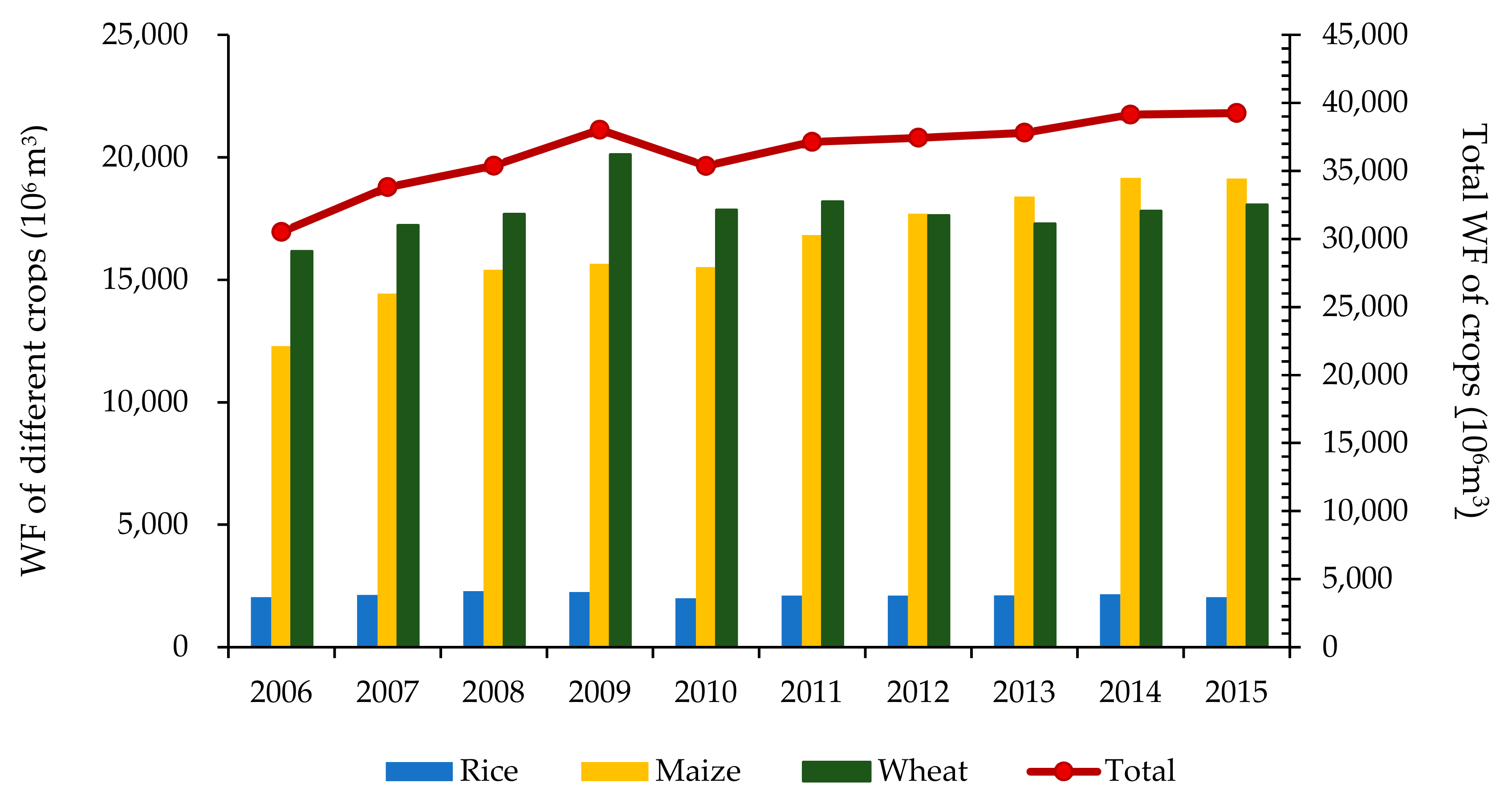
As shown in Figure 2, the total WF of crops in Northwest China experienced a general increasing trend from 2006 to 2015. The total WF increased from 30,506.41 (106 m3) in 2006 to 39,521.64 (106 m3) in 2015, with an average annual growth rate of 2.84%. Specifically, the composition of the total WF of the three staple foods also changed significantly. In 2006, the WF of maize accounted for 40.30% of the total WF; however, this value rose to a peak of 48.96% in 2014. At the same time, the proportion of the WF attributed to wheat decreased gradually during the study period, from 53% in 2006 to 45.50% in 2014. Since rice is not a major crop in these five northwestern provinces and regions, in comparison to those of the other two crops, the WF of rice has always been low, and it changed imperceptibly, with an average proportion of 5.87%.
3.2. Decomposition Analysis from the Perspective of Time
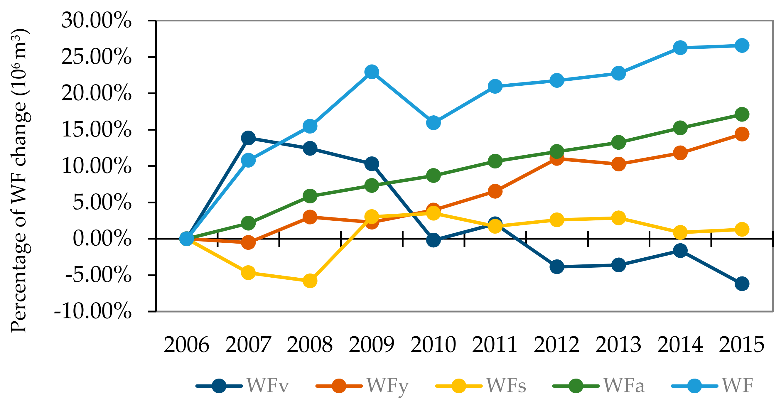
We decomposed the changes of the total WF of crops in the five northwestern provinces and regions from 2006 to 2015 into four effects: the VWC effect, yield effect, crop structure effect, and crop area effect, or WFv, WFy, WFs, and WFa, respectively. As shown in Figure 3, the crop area and yield effects were positive effects that led to an increase in the overall WF of the crops from 2006 to 2015. During the study period, the crop area effect in absolute terms was always positive, while the yield effect was also mainly positive, with 8 out of 9 years showing positive values. The VWC effects changed from positive factors that contributed to the overall increase to negative factors that inhibited such an increase with high volatility, and the VWC effects had negative values in 5 years, totaling −9208.55 (106 m3), and positive values in 4 years, totaling 5862.79 (106 m3). The overall effect of the VWC from 2006 to 2015 was −3345.77 (106 m3), indicating that it inhibited the overall increase of the WF. On the other hand, the impact of the crop structure effect was relatively small, fluctuating sharply between 2006 and 2010, but tended to be stable between 2010 and 2015, producing a gradually weakening inhibition impact on the overall increase. Therefore, in general, the WF reduction due to the VWC and planting structure did not offset the increase in the WF originating from the effects of the crop area and yield. Therefore, the total WF of crops in five northwestern provinces and regions in China showed an increasing trend during the study period.
3.2.1. Virtual Water Content Effect
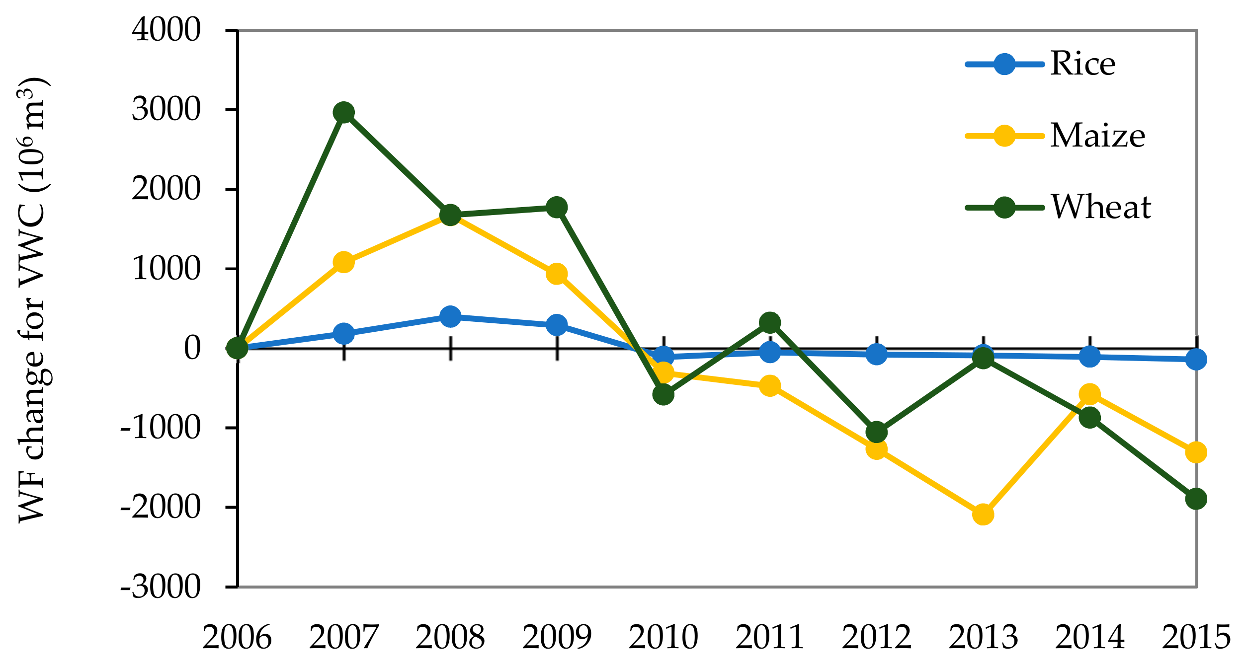
Figure 3 and Figure 4 show that the VWC effect played a significant role in changing the overall WF of the crops in the five northwestern provinces and regions. Wheat, as the main food crop in Northwest China, had the highest contribution, and its total VWC effect reached −1896.21 (106 m3), accounting for 56.68% of the three staple foods. Maize had the next-highest contribution, with a total effect of 1309.5 (106 m3), accounting for 39.14% of the three staple foods. The contribution of the rice VWC effect was the lowest because rice is relatively water-intensive, so it is not suitable for planting in the five northwestern provinces and regions in China. In addition, Figure 3 further illustrates the significant impact of the VWC on the WF, as climatic factors (such as temperature, sunlight and sunshine, and precipitation) and natural features (latitude, longitude, and altitude) changed the crop yield and associated water consumption during the study period. For example, in a study of rice in Sri Lanka, Silva et al. concluded that climate change impacts the demand for irrigation water and the water balance in Sri Lanka [36]. Therefore, calculating the WF using the multi-year average VWC of crops in the past, such as in the study conducted by Liu et al. [37], would lead to calculation bias and affect the research results.
3.2.2. Crop Area Effect
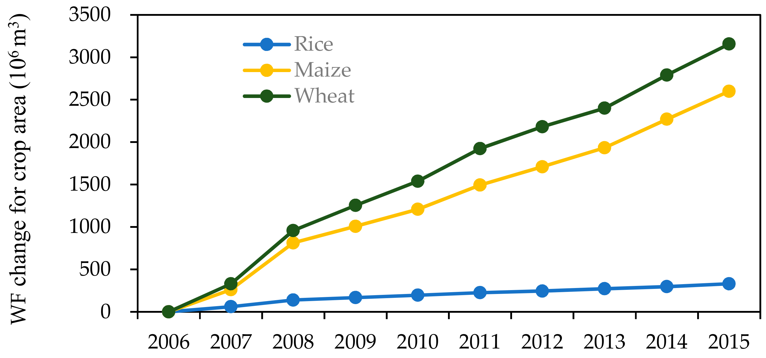
Figure 5 shows that the cumulative contribution of the crop area effect to the WF steadily increased, contributing the most to the overall increase, and its curve was consistent with the curve of the overall WF for crops. From 2006 to 2009, the WF increased sharply with the crop area effect, but in 2010, due to the inhibition effect of the VWC, the WF decreased from 38,020.78 (106 m3) to 35,362.31 (106 m3). Since 2011, the WF has risen modestly under the significant influence of the crop area effect. The above changes were correlated with changes in the planting areas of various crops in Northwest China. Between 2006 and 2010, the planting area of the five northwestern provinces and regions showed a steady and moderate upward trend, from 13.45 million ha in 2006 to 16.09 million ha in 2015, with an average annual growth rate of 2.02%, which stimulated the increased WF. As shown in Figure 4, the crop area effect of wheat had the highest contribution to the overall increased WF among the three staple crops, followed by maize and rice, which was consistent with the planting structure of the five northwestern provinces and regions.
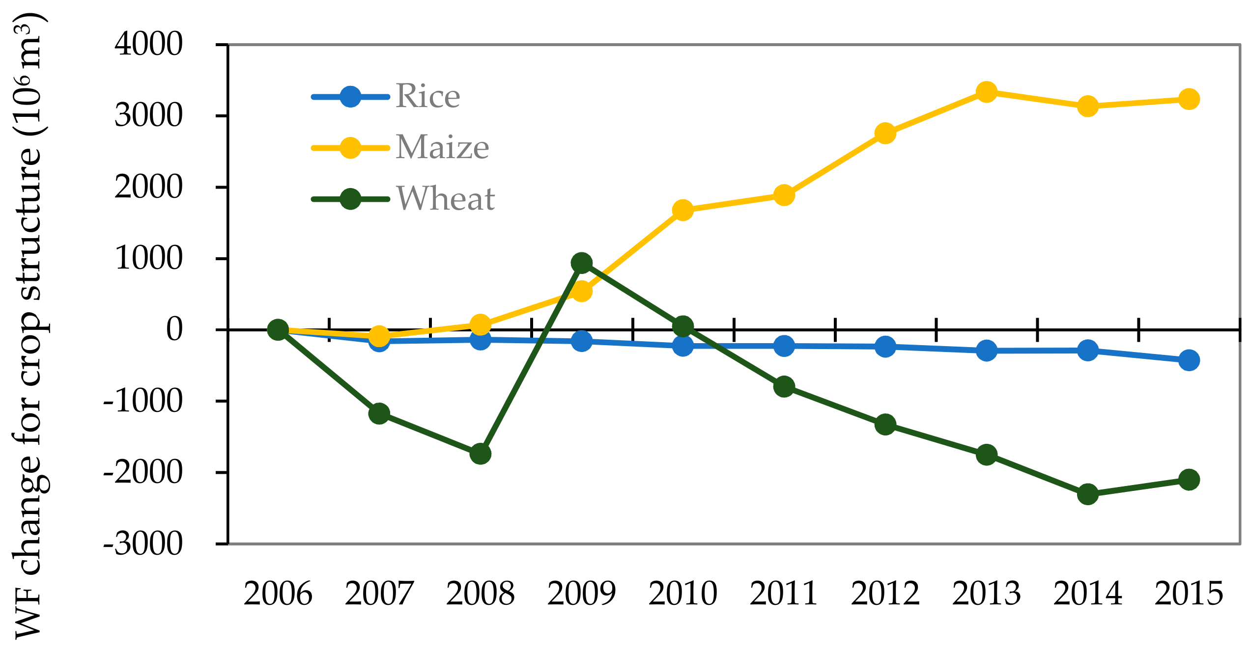
3.2.3. Crop Structure Effect
In general, compared with the contribution of the VWC effect and crop area effect to WF, the overall effect of the planting structure on the crop WF was small during the study period, the cumulative contribution of which only accounted for 8.05% of the total effect. Specifically, as shown in Figure 6, the proportion of wheat planting area among the major crop areas decreased between 2006 and 2015, from an average planting rate of 24.97% in 2006 to 18.22% in 2015. The area proportion of maize increased from 14.38% to 19.27%. This change was particularly evident in Gansu, Qinghai, and Ningxia. As a result, the decreasing crop area proportion of wheat inhibited the increased WF, while the increasing crop area proportion of maize contributed to the increased WF, which led to a canceling effect between the positive and negative values.
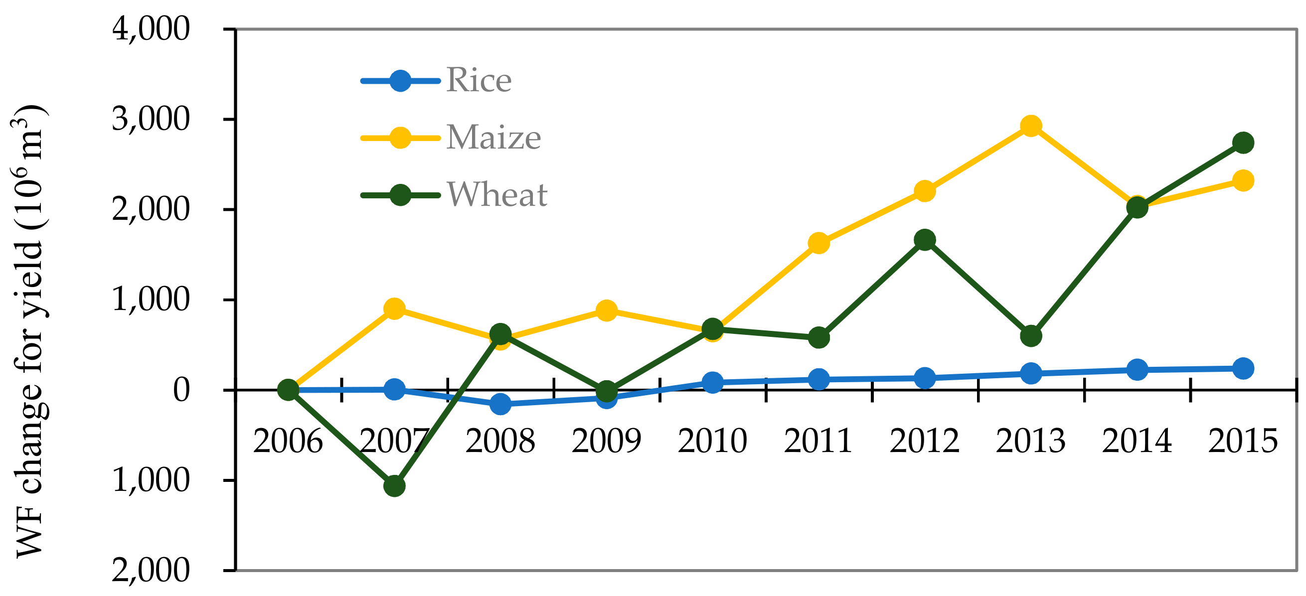
3.2.4. Yield Effect
From 2006 to 2015, the WF in the five northwestern provinces and regions generally increased with increased yields of crops. The yield effects in absolute terms were positive except in 2007, 2009, and 2013, and in general, the WF showed a change in volatility from a decrease to an increase. As shown in Figure 7, the yield effect of wheat contributed the most to the change in the WF, from 7740.39 (kg/ha) in 2006 to 4098.92 (kg/ha) in 2015, with an average annual increase of 1.02%, driving the WF to increase to 2709.95 (106 m3); corn had the second-greatest contribution, driving the WF to increase to 2320.16 (106 m3), while the contribution of rice was the smallest, driving the WF to increase to 238.50 (106 m3).
3.3. Total Water Footprint (WF) in Different Provinces and Regions
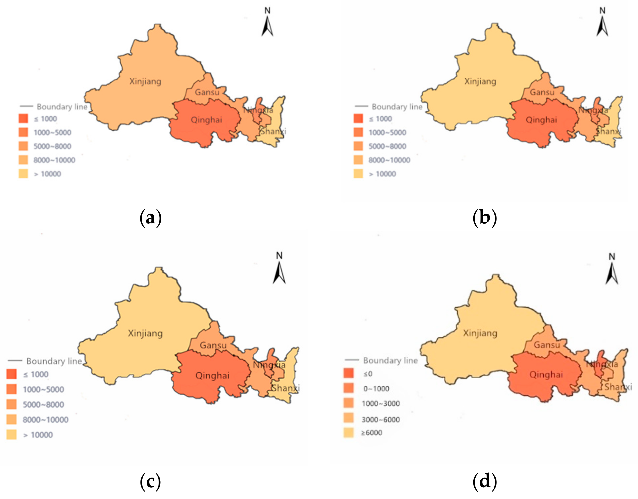
As shown in Figure 8, from 2006 to 2015, the overall WF of the crops in the five northwestern provinces and regions showed an increasing trend but remarkable spatial disparity. The WF in Shanxi was always the greatest, and the WF in Qinghai was the lowest. Compared with the WF in 2006, the WF values in 2010 in Shaanxi, Gansu, and Xinjiang increased, among which Xinjiang had the most significant increase, reaching 5397.14 (106 m3) and accounting for 61.71% of the total increase in these five provinces and regions. This result further indicated a trend exceeding that of Shaanxi. Qinghai’s and Ningxia’s WF declined gently, which had little effect on the overall WF, accounting for only −1.73% and −3.65%, respectively. In general, the change in the WF in the five northwestern provinces and regions showed a trend of “high-low-high” from west to east in the study period. The grain production statuses of Xinjiang and Shaanxi further improved, while the statuses of Ningxia and Qinghai in the central region declined.
3.4. Decomposition Analysis from the Perspective of Space
During the study period, the WF in Shaanxi was the largest among the five northwestern provinces and regions with relatively high growth rates. Therefore, we considered the WF in Shaanxi as the control group and the WFs in other smaller provinces and regions as the comparison group. Then, we compared the WFs among the provinces and regions. According to Equations (15)–(19), we calculated the driving effects and contribution rates for the spatial differences in the WFs in Northwest China from 2006 to 2015, as shown in Table 1.
3.4.1. Gansu-Shanxi
In 2006, 2010, and 2015, the WF in Gansu was 4756.43 (106 m3), 6702.94 (106 m3), and 6380.74 (106 m3), respectively, which was less than that in Shaanxi, and had an increasing trend, with the overall increasing trend being Shaanxi was clearer. Specifically, the VWC effect in absolute terms was positive in 2006 and negative in 2010 and 2015, indicating that the VWC effects on the WF increase in Gansu were first stronger than that in Shaanxi and then weaker, and the gap gradually widened. The yield effect was negative in 2006 and 2010 and positive in 2015, indicating that the contribution of the yield effects to the WF increase in Gansu was stronger than that in Shaanxi. The structure effect and land area effect in absolute terms were always negative, indicating that the contributions of these effects to the WF increase in Gansu were weaker than those in Shaanxi but had a narrowed gap.
3.4.2. Qinghai-Shanxi
In 2006, 2010, and 2015, the WF in Qinghai was 10,345.35 (106 m3), 12,916.74 (106 m3), and 13,048.15 (106 m3), respectively, which was less than that in Shaanxi and showed a significant increasing trend. The overall WF in Qinghai was the lowest among the WFs of the five provinces and regions during the study period, and no rice was planted there. In addition, the planting area and yield of corn and wheat were also small. Specifically, the VWC effect in absolute terms was always negative, indicating that the VWC effects on the WF increase in Qinghai were weaker than those in Shaanxi, and the gap gradually widened. The yield effects were always positive, indicating that the contribution of the yield effects to the WF increase in Qinghai was stronger than that in Shaanxi but with great fluctuations. The structure effect and land area effect in absolute terms were always negative with high values, indicating that the contributions of these effects to the WF increase in Qinghai were weaker than those in Shanxi, but the gap narrowed.
3.4.3. Ningxia-Shanxi
In 2006, 2010, and 2015, the WF in Ningxia was 8684.23 (106 m3), 11,520.94 (106 m3), and 11,725.23 (106 m3), respectively, which was less than that in Shaanxi and showed a significantly increasing trend. The overall increasing trend of the WF in Shaanxi was clearer, and the planting areas of the three food crops in Ningxia were also much smaller than those in Shaanxi. Specifically, the VWC effect in absolute terms was always negative, indicating that the VWC effects on the WF increase in Ningxia were weaker than those in Shaanxi, with a fluctuating increasing trend. The yield effect was positive, indicating that the contribution of yield effects to the WF increase in Ningxia was stronger than that in Shaanxi, but the gap gradually narrowed. The structural effect and the crop area effect were always negative, indicating that the contributions of these effects to the WF increase in Ningxia were weaker than those in Shanxi, which was the main driving factor causing the difference between the WF in Ningxia and Shaanxi.
3.4.4. Xinjiang-Shanxi
In 2006, 2010, and 2015, the WF in Xinjiang was 3584.37 (106 m3), 3805.45 (106 m3), and 908.76 (106 m3), respectively, which was less than that in Shaanxi and showed a decreasing trend. The growth rate of the WF in Xinjiang gradually surpassed that in Shaanxi during the study period. Specifically, the VWC effect in absolute terms was always negative, indicating that the VWC effects on the WF increase in Xinjiang were weaker than those in Shaanxi, and the gap gradually widened. Additionally, the VWC provided a good complement, offering further insights into the influence of regional differences and climate change on the water demand [20]. The yield effect was positive, indicating that the contribution of the yield effect to the WF increase in Xinjiang was stronger than that in Shaanxi and was the main driving factor behind the growth of the WF in Xinjiang. The structural effect was always negative, indicating that the contribution of this effect to the WF increase in Ningxia was weaker than that in Shanxi, but the gap narrowed. The effect of the crop area was always positive and gradually increased, indicating that the contribution of the crop area effect to the WF increase in Ningxia was weaker than that in Shanxi.
4. Conclusions
4.1. Assessing the Ensemble Result of the Driving Effects
We set out to identify the drivers of the WF of grain crops, focusing on the VWC, yield, crop structure, and crop area. The results can be described from two different perspectives, as follows:
From the perspective of the changes in the WF over time, the expansion of the cultivated land area and increase of the unit yield were the major driving factors behind the increase in the WF in Northwest China from 2006 to 2015, especially the increase in cultivated land area. Since the cultivated land area increased steadily with an annual growth rate of 2.02% during the study period in Northwest China, the WF increased consistently with the expansion of the cultivated land area. The change in the VWC also played a significant role in the increased WF and changed from an effect that inhibited the WF increase at the beginning of the study to the effect that contributed to the increase. This scenario occurred because, during the study period, many policies related to water conservation were implemented to lower the VWC per unit, while the contribution of the crop structure effect was less than those of other effects to the WF. Although the food consumption pattern in China changed slightly over the study period, crop, maize, and wheat are still the staple food crops in China. Therefore, there was only a minor adjustment within the crop structure, which led to a canceling effect of the increase in the planting area of maize and the decrease in the area of wheat.
From the perspective of the changes in the WF spatially, the WFs in the five northwestern provinces and regions showed a trend of “high-low-high” from west to east from 2006 to 2015, with the largest WF in Shanxi and the smallest in Qinghai. The VWC effects contributed significantly to increasing the differences among the provinces and regions due to the unbalanced distribution of land, light, and heat resources among these areas. The crop structure and crop area effect were also important factors since the water requirement of wheat was the largest among the three crops, and an increase in the production of wheat was a significant driving factor behind the increase in the WF. In addition, the yield effect was the main driving factor promoting WF growth in Xinjiang due to the construction of high-quality farmland, which led to significant growth of the yield in Xinjiang, indicating that the WF in Xinjiang would gradually surpass that in Shaanxi.
4.2. Implications for Conserving Agricultural Water in Northwest China
Although China’s water use efficiency in the agricultural sector improved over the study period, the water use efficiency is still low when compared with those of other industrialized countries due to inappropriate irrigation management practices and lower investments in infrastructure construction [38]. However, our result doesn’t simply mean that the regions with a low WF should produce more to increase the water use efficiency. The poor natural endowment will lead regions with less water to save more, like improving the water use efficiency by changing irrigation methods, among implementing other changes, so that the blue water footprint will be reduced. But for future consideration and the sustainable use of water, it is not appropriate to arrange high production for regions with less water, considering their natural endowment, since it will lower the environmental carrying capacity eventually. Therefore, a different approach should be taken.
To date, China has gradually carried out campaigns to control water in agriculture sectors from the perspective of supply through water resource reallocation, water pricing, etc. The fact that the VWC values of rice, maize, and wheat were different in different years and the contribution of the crop structure effect to the improved WF in Northwest China, as found in our study, justify the significance of the VWC, we thought it is important to plan and arrange crop planting structures reasonably based on science to control the total WF in Northwest China. In addition, virtual water trade, which allows water-scarce areas to import water-intensive products from water-rich areas, should also be utilized to further improve the efficiency of agricultural water use since this approach can alleviate water shortages in the five northwestern provinces and regions to a certain extent [39]. The grain planting structure, geographical environment, and climate in the five northwestern provinces and regions are similar. However, during the study period, there was a remarkable spatial disparity among the provinces and regions in Northwest China. To achieve a spatial balance, home-grown and grass-roots solutions are needed. For the provinces and regions with large WFs that are under conditions of comparatively good light and heat, such as Shanxi and Xinjiang, it is time to reduce the water and fertilizer application properly [40] and apply linear programming as opposed to simply expanding the cultivated area [41]. In addition, Gansu experiences a challenge involving the shortage of water resources and the high proportion of agriculture in its GDP. Therefore, it is necessary to reallocate the structure of the food and animal husbandry sectors. Provinces and regions that lack water and have a fragile ecological environment, such as Gansu, Ningxia, and Qinghai in Northwest China, are unable to meet the needs for the growth of some crops. Therefore, it is time to abandon broad-scale expansion and emphasize the quality of agricultural development. The yield effect of crops greatly contributes to the changes in the WFs, so we should promote advanced agricultural science and skills to improve the yield of each grain crop to lower the total WF in agricultural production. Furthermore, attention should be paid to strengthening the construction of high-quality farmland.
Author Contributions
Conceptualization, C.S.; Methodology, Y.W.; Supervision, C.Z. and L.Z.
Funding
This research was supported by the National Natural Science Foundation of China (Grant Numbers: 41701613), the Humanities and Social Sciences Foundation of Ministry of Education in China (Grant Numbers: 17YJC790194), and the Fundamental Research Funds for the Central Universities (Grant Numbers:2019B23014).
Conflicts of Interest
The authors declare no conflict of interest.
References
- Cao, X.; Pute, W.U.; Wang, Y.; Zhao, X. Water Footprint of Grain Product in Irrigated Farmland of China. Water Resour. Manag. 2014, 28, 2213–2227. [Google Scholar] [CrossRef]
- Qin, L.; Jin, Y.; Duan, P.; He, H. Field-based Experimental Water Footprint Study of Sunflower Growth in a Semiarid Region of China. J. Sci. Food Agric. 2016, 96, 3266–3273. [Google Scholar] [CrossRef] [PubMed]
- Joshua, E.; Delphine, D.; Christoph, M.; Katja, F.; Markus, K.; Dieter, G.; Michael, G.; Martina, F.R.; Yoshihide, W.; Neil, B. Constraints and potentials of future irrigation water availability on agricultural production under climate change. Proc. Natl. Acad. Sci. USA 2014, 111, 3239–3244. [Google Scholar]
- Shtull-Trauring, E.; Bernstein, N. Virtual water flows and water-footprint of agricultural crop production, import and export: A case study for Israel. Sci. Total Environ. 2018, 622, 1438–1447. [Google Scholar]
- Wu, X.; Degefu, D.M.; Yuan, L.; Liao, Z.; He, W.; An, M.; Zhang, Z. Assessment of Water Footprints of Consumption and Production in Transboundary River Basins at Country-Basin Mesh-Based Spatial Resolution. Int. J. Environ. Res. Public Health 2019, 16, 703. [Google Scholar] [CrossRef]
- Chapagain, A.K.; Hoekstra, A.Y.; Savenije, H.H.G. Water saving through international trade of agricultural products. Hydrol. Earth Syst. Sci. 2006, 10, 455–468. [Google Scholar] [CrossRef]
- Sun, C.Z.; Liu, Y.Y.; Chen, L.X.; Zhang, L. The spatial-temporal disparities of water footprints intensity based on Gini coefficient and Theil index in China. Acta Ecol. Sin. 2010, 30, 1312–1321. [Google Scholar]
- Gonzalez Perea, R.; Camacho Poyato, E.; Montesinos, P.; Garcia Morillo, J.; Rodriguez Diaz, J.A. Influence of spatio temporal scales in crop water footprinting and water use management: Evidences from sugar beet production in Northern Spain. J. Clean. Prod. 2016, 139, 1485–1495. [Google Scholar] [CrossRef]
- Sun, S.K.; Wu, P.T.; Wang, Y.B.; Zhao, X.N. The virtual water content of major grain crops and virtual water flows between regions in China. J. Sci. Food Agric. 2013, 93, 1427–1437. [Google Scholar] [CrossRef]
- Bulsink, F.; Hoekstra, A.Y.; Booij, M.J. The water footprint of Indonesian provinces related to the consumption of crop products. Hydrol. Earth Syst. Sci. 2010, 14, 119–128. [Google Scholar] [CrossRef]
- Yao, L.; Xu, J.; Zhang, L.; Pang, Q.; Zhang, C. Temporal-spatial decomposition computing of regional water intensity for Yangtze River Economic Zone in China based on LMDI model. Sustain. Comput. Inform. Syst. 2019, 21, 119–128. [Google Scholar] [CrossRef]
- Zou, M.; Kang, S.; Niu, J.; Lu, H. A new technique to estimate regional irrigation water demand and driving factor effects using an improved SWAT model with LMDI factor decomposition in an arid basin. J. Clean. Prod. 2018, 185, 814–828. [Google Scholar] [CrossRef]
- Bruneau, J.F.; Renzetti, S. Water Use Intensities and the Composition of Production in Canada. J. Water Resour. Plan. Manag. 2010, 136, 72–79. [Google Scholar] [CrossRef]
- Zhi, Y.; Yang, Z.; Yin, X.-A.; Hamilton, P.B.; Zhang, L. Evaluating and Forecasting the Drivers of Water Use in a City: Model Development and a Case from Beijing. J. Water Resour. Plan. Manag. 2016, 142, 04015042. [Google Scholar] [CrossRef]
- Ma, J.; Wang, D.; Lai, H.; Wang, Y. Water Footprint—An Application in Water Resources Research. Resour. Sci. 2005, 27, 96–100. [Google Scholar]
- Yang, H.; Pfister, S.; Bhaduri, A. Accounting for a scarce resource: Virtual water and water footprint in the global water system. Curr. Opin. Environ. Sustain. 2013, 5, 599–606. [Google Scholar] [CrossRef]
- Chunfu, Z.; Bin, C. Driving force analysis of the agricultural water footprint in China based on the LMDI method. Environ. Sci. Technol. 2014, 48, 12723–12731. [Google Scholar]
- Zhao, X.; Tillotson, M.R.; Liu, Y.W.; Guo, W.; Yang, A.H.; Li, Y.F. Index decomposition analysis of urban crop water footprint. Ecol. Model. 2017, 348, 25–32. [Google Scholar] [CrossRef]
- Xu, Y.; Kai, H.; Yu, Y.; Wang, X. Changes in water footprint of crop production in Beijing from 1978 to 2012: A logarithmic mean Divisia index decomposition analysis. J. Clean. Prod. 2015, 87, 180–187. [Google Scholar] [CrossRef]
- Deng, G.; Xu, Y.; Yu, Z. Accounting and change trend analysis of food production water footprint in China. Water Policy 2018, 20, 758–776. [Google Scholar] [CrossRef]
- Cheng, G.D.; Zhao, W.Z. Green Water and Its Research Progresses. Adv. Earth Sci. 2006, 21, 221–227. [Google Scholar]
- Hoekstra, A.Y.; Chapagain, A.K. Water footprints of nations: Water use by people as a function of their consumption pattern. Water Resour. Manag. 2007, 21, 35–48. [Google Scholar] [CrossRef]
- Chapagain, A.K.; Hoekstra, A.Y. The blue, green and grey water footprint of rice from production and consumption perspectives. Ecol. Econ. 2011, 70, 749–758. [Google Scholar] [CrossRef]
- Mekonnen, M.M.; Hoekstra, A.Y. The green, blue and grey water footprint of crops and derived crop products. Hydrol. Earth Syst. Sci. 2011, 15, 1577–1600. [Google Scholar] [CrossRef]
- Pute, W.U.; Sun, S.; Wang, Y.; Xiaolei, L.I.; Zhao, X. Research on the quantification methods for water footprint of crop production. J. Hydraul. Eng. 2017, 48, 651–660 and 669. [Google Scholar]
- Sun, S.; Wu, P.; Wang, Y.; Zhao, X.; Liu, J.; Zhang, X. The impacts of interannual climate variability and agricultural inputs on water footprint of crop production in an irrigation district of China. Sci. Total Environ. 2013, 444, 498–507. [Google Scholar] [CrossRef]
- Egan, M. The Water Footprint Assessment Manual. Setting the Global Standard. Soc. Environ. Account. J. 2011, 31, 181–182. [Google Scholar] [CrossRef]
- Wang, C.; Chen, J.N.; Zou, J. Decomposition of energy-related CO2 emission in China: 1957–2000. Energy 2005, 30, 73–83. [Google Scholar] [CrossRef]
- Hatzigeorgiou, E.; Polatidis, H.; Haralambopoulos, D. CO2 emissions in Greece for 1990–2002: A decomposition analysis and comparison of results using the Arithmetic Mean Divisia Index and Logarithmic Mean Divisia Index techniques. Energy 2008, 33, 492–499. [Google Scholar] [CrossRef]
- Ang, B.W. Decomposition analysis for policymaking in energy: Which is the preferred method? Energy Policy 2004, 32, 1131–1139. [Google Scholar] [CrossRef]
- Zhang, S.L.; Su, X.L.; Singh, V.P.; Olaitan, A.O.; Xie, J. Logarithmic Mean Divisia Index (LMDI) decompositionanalysis of changes in agricultural water use: A case study of the middle reaches of the Heihe River basin, China. Agric. Water Manag. 2018, 208, 422–430. [Google Scholar] [CrossRef]
- Zhang, L.; Dong, H.J.; Geng, Y.; Francisco, M.J. China’s provincial grey water footprint characteristic and driving forces. Sci. Total Environ. 2019, 677, 427–435. [Google Scholar] [CrossRef] [PubMed]
- Gao, W.; Howarth, R.W.; Swaney, D.P.; Hong, B.G.; Guo, H.C. Enhanced N input to Lake Dianchi Basin from 1980 to 2010: Drivers and consequences. Sci. Total Environ. 2015, 505, 376–384. [Google Scholar] [CrossRef] [PubMed]
- Li, Y.; Lu, L.Y.; Tan, Y.X.; Wang, L.L.; Shen, M.H. Decoupling Water Consumption and Environmental Impact on Textile Industry by Using Water Footprint Method: A Case Study in China. Water 2017, 9, 124. [Google Scholar] [CrossRef]
- Silva, C.S.D.; Weatherhead, E.K.; Knox, J.W.; Rodriguez-Diaz, J.A. Predicting the impacts of climate change—A case study of paddy irrigation water requirements in Sri Lanka. Agric. Water Manag. 2007, 93, 19–29. [Google Scholar] [CrossRef]
- Liu, J.; Zehnder, A.J.B.; Yang, H. Historical Trends in China’s Virtual Water Trade. Water Int. 2007, 32, 78–90. [Google Scholar] [CrossRef]
- Miguel, Á.D.; García, E.; Buestamante, I.D. Estimation of the virtual water trade between two Spanish regions: Castilla-la Mancha and Murcia. Water Sci. Technol. Water Supply 2010, 10, 831–840. [Google Scholar] [CrossRef]
- Yang, G.; He, X.L.; Zheng, T.G.; Maina, J.N.; Li, J.F.; Liu, H.L. Integrated agricultural irrigation management technique in the arid inland area, China. J. Food Agric. Environ. 2012, 10, 736–741. [Google Scholar]
- Zhang, Y.; Zhang, J.; Tang, G.; Chen, M.; Wang, L. Virtual water flows in the international trade of agricultural products of China. Sci. Total Environ. 2016, 557, 1–11. [Google Scholar] [CrossRef]
- Aguilera, E.; Lassaletta, L.; Sanz-Cobena, A.; Garnier, J.; Vallejo, A. The potential of organic fertilizers and water management to reduce N 2 O emissions in Mediterranean climate cropping systems. A review. Agric. Ecosyst. Environ. 2013, 164, 32–52. [Google Scholar] [CrossRef] [Green Version]
- Pongpinyopap, S.; Mungcharoen, T. Bioethanol water footprint: Life cycle optimization for water reduction. Water Sci. Technol. Water Supply 2015, 15, 395. [Google Scholar] [CrossRef]
Figure 1.
Land cover map of the research area.

Figure 2.
Total WF (water footprint) of crops and its composition in Northwest China (2006–2015).

Figure 3.
Driving forces of the total WF for the crops during the study period of 2006–2015.

Figure 4.
The cumulative contribution of the virtual water content to the WF change.

Figure 5.
The cumulative contribution of crop area to WF change.

Figure 6.
The cumulative contribution of the crop structure to the WF change.

Figure 7.
The cumulative contribution of the yield effect to the WF change.

Figure 8.
The total WF of crops and its changes from 2006 to 2015. (a) Total WF of crops in 2006; (b) Total WF of crops in 2010; (c) Total WF of crops in 2015; (d) Change in WF during 2006–2015.
Figure 8.
The total WF of crops and its changes from 2006 to 2015. (a) Total WF of crops in 2006; (b) Total WF of crops in 2010; (c) Total WF of crops in 2015; (d) Change in WF during 2006–2015.


Table 1.
Driving effects and contribution rates of the spatial differences in the WFs in Northwest China from 2006 to 2015 (106 m3).
Table 1.
Driving effects and contribution rates of the spatial differences in the WFs in Northwest China from 2006 to 2015 (106 m3).
| Provinces | Year | WFv | WFy | WFs | WFa | Total Effect |
|---|---|---|---|---|---|---|
| Gansu-Shanxi | 2006 | 730.47 | −814.39 | −3909.69 | −762.83 | −4756.43 |
| −15.36% | 17.12% | 82.20% | 16.04% | 100.00% | ||
| 2010 | −1934.19 | −836.72 | −3447.40 | −484.64 | −6702.94 | |
| 28.86% | 12.48% | 51.43% | 7.23% | 100.00% | ||
| 2015 | −3488.75 | 211.43 | −2963.61 | −139.80 | −6380.74 | |
| 54.68% | −3.31% | 46.45% | 2.19% | 100.00% | ||
| 2006 | −1457.79 | 832.38 | −3608.23 | −6111.72 | −10,345.35 | |
| 14.09% | −8.05% | 34.88% | 59.08% | 100.00% | ||
| Qinghai-Shanxi | 2010 | −2468.22 | 1011.40 | −4321.00 | −7138.93 | −12,916.74 |
| 19.11% | −7.83% | 33.45% | 55.27% | 100.00% | ||
| 2015 | −2154.16 | 421.56 | −3775.10 | −7540.45 | −13,048.15 | |
| 16.51% | −3.23% | 28.93% | 57.79% | 100.00% | ||
| 2006 | −796.04 | 1710.96 | −1493.70 | −8105.45 | −8684.23 | |
| 9.17% | −19.70% | 17.20% | 93.34% | 100.00% | ||
| Ningxia-Shanxi | 2010 | −2531.45 | 1596.71 | −2283.03 | −8303.18 | −11,520.94 |
| 21.97% | −13.86% | 19.82% | 72.07% | 100.00% | ||
| 2015 | −2141.53 | 1115.56 | −2305.43 | −8393.83 | −11,725.23 | |
| 18.26% | −9.51% | 19.66% | 71.59% | 100.00% | ||
| 2006 | −2721.68 | 4994.13 | −6321.59 | 464.77 | −3584.37 | |
| 75.93% | −139.33% | 176.37% | −12.97% | 100.00% | ||
| Xinjiang-Shanxi | 2010 | −5141.07 | 4949.70 | −5178.35 | 1560.27 | −3809.45 |
| 134.96% | −129.93% | 135.93% | −40.96% | 100.00% | ||
| 2015 | −5207.30 | 4996.13 | −4819.70 | 4122.10 | −908.76 | |
| 573.01% | −549.77% | 530.36% | −453.60% | 100.00% |
WFv, WFy, WFs, and WFa represent the VWC effect, yield effect, crop structure effect, and crop area effect respectively.
© 2019 by the authors. Licensee MDPI, Basel, Switzerland. This article is an open access article distributed under the terms and conditions of the Creative Commons Attribution (CC BY) license (http://creativecommons.org/licenses/by/4.0/).
Share and Cite
MDPI and ACS Style
Shi, C.; Wang, Y.; Zhang, C.; Zhang, L. Spatial-Temporal Differences in Water Footprints of Grain Crops in Northwest China: LMDI Decomposition Analysis. Water 2019, 11, 2457. https://doi.org/10.3390/w11122457
AMA Style
Shi C, Wang Y, Zhang C, Zhang L. Spatial-Temporal Differences in Water Footprints of Grain Crops in Northwest China: LMDI Decomposition Analysis. Water. 2019; 11(12):2457. https://doi.org/10.3390/w11122457
Chicago/Turabian StyleShi, Changfeng, Yanying Wang, Chenjun Zhang, and Lina Zhang. 2019. "Spatial-Temporal Differences in Water Footprints of Grain Crops in Northwest China: LMDI Decomposition Analysis" Water 11, no. 12: 2457. https://doi.org/10.3390/w11122457
Note that from the first issue of 2016, this journal uses article numbers instead of page numbers. See further details here.