Streamflow Variability in Mahaweli River Basin of Sri Lanka during 1990–2014 and Its Possible Mechanisms


1
International Center for Climate and Environment Sciences, Institute of Atmospheric Physics, Chinese Academy of Sciences, P.O. Box 9804, Beijing 100029, China
2
University of Chinese Academy of Sciences, Beijing 100049, China
3
Collaborative Innovation Center on Forecast and Evaluation of Meteorological Disasters, Nanjing University of Information Science and Technology, Nanjing 210044, China
*
Author to whom correspondence should be addressed.
Water 2019, 11(12), 2485; https://doi.org/10.3390/w11122485
Submission received: 7 October 2019
/
Revised: 15 November 2019
/
Accepted: 19 November 2019
/
Published: 25 November 2019
(This article belongs to the Section Hydrology)
Abstract
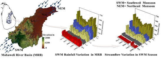
:This study investigates the variation of seasonal streamflow and streamflow extremes in five catchments of the Mahaweli River Basin (MRB) Sri Lanka from 1990 to 2014, and the relationship between streamflow and seasonal rainfall in each catchment is then examined. Furthermore, the influence of Indian Ocean Dipole (IOD) and El Nino and Southern Oscillation (ENSO) on the seasonal rainfall and streamflow in the upper (UMRB) and lower reaches (LMRB) of MRB are explored. It’s found that the rainfall amount in southwest monsoon (SWM) season contributes 29.7% out of annual total rainfall in the UMRB, while the LMRB records 41% of the total rainfall during the northeast monsoon (NEM) season. The maximum streamflow of upper (lower) Mahaweli catchments is observed in the SWM (NEM) season. Catchments in the UMRB (LMRB) recorded strong interannual variability of seasonal overall flow (Q50), Maximum 10-day, and 30-day flows during the SWM (NEM) season. It’s further revealed that the catchment streamflow in the UMRB is closely correlated with the SWM rainfall in the interannual time scale, while streamflow of catchments in the LMRB is closely associated with the NEM rainfall. The effects of ENSO and IOD on streamflow are consistent with their impacts on rainfall for all catchments in MRB, with strong seasonal dependent. These suggested that the sea surface temperature anomalies in the both Indian Ocean and tropical Pacific Ocean are important factors affecting the streamflow variability in the MRB, especially during the SWM season.
1. Introduction
The hydrologic cycle at the watershed scale reflects the complex interactions among climate, land use, and land cover changes (LULC), soil properties, geology, and terrain [1]. Climate change affects the changes in the global hydrological cycle [2] that can lead to severe storms, floods, and droughts [3]. Streamflow is the most important component of the hydrological cycle, which directly links to water resources management. Alterations in the long-term discharge of streamflow can be caused by decadal or inter-decadal climate variability, and anthropogenic activates such as LULC in the upstream basin, construction of reservoirs [4], and diversion of water for irrigation [5,6]. Among them, precipitation variability [7] and LULC [8] in the watershed are the two most likely drivers of long-term discharge modifications in a large river basin. For example, Pascolini-Campbell et al. [9] found that natural precipitation variability influenced by interannual to decadal ENSO variability is the main cause for observed inter-annual variability of Gila River flow. Similarly, Panda et al. [10] revealed that intensified interannual variability of the Mahanadi streamflow is occurred due to the moving variability of rainfall. Furthermore, stronger interannual rainfall signals showed the same pattern as the streamflow variability over West Africa [11]. These facts suggested that annual and seasonal variations in the streamflow associated with the inconsistent atmospheric conditions via variation in rainfall and temperature. The resulting anomalous flow regimes may have caused a series of water resource problems in some regions [12], in terms of quality and quantity [13]. In these situations, altered flow regimes affect hydropower generation, drainage, and irrigation operation [14] as well as freshwater ecosystems. Therefore, the impacts of climate change and anthropogenic perturbations on changes in the streamflow [15] have been widely investigated by the research community in recent years.
As a result of climate change, the earlier studies of streamflow in various parts of the world observed either increased river discharge [5,16] or increased water stress [17]. In addition, some studies identified the changes in streamflow in different seasons [10,18]. Observational studies revealed a decreasing trend in annual flood maxima, despite increases in precipitation [19]. Wasko and Sharma [20] reported that a rise in temperature could cause a rise in precipitation, which leads to an overall increase in streamflow at small catchments. Gudmundsson et al. [21] found that significantly decreasing regional trend in mean, 90th percentile of streamflow, and maximum streamflow in South Asia for the period of 1971–2010 while the observed increasing trend of these streamflow variables in East Asia for the period of 1961–2000. Zhang et al. [22] reported declining trends of streamflow in southern Australia since 1950. Based on these studies, the trend and variability of the streamflow are not the same around the world, which could be largely ascribed to the difference in rainfall trends and variations.
The Mahaweli Development Program (MDP) was implemented based on the Mahaweli River Basin (MRB) since 1977. As the largest and the most extensive physical and human resource development program ever implemented in Sri Lanka, MDP had focused on constructing a series of reservoirs, hydroelectricity plants and to develop a large area of land with irrigation. After implementing MDP, Mahaweli water irrigates in the one-sixth (55% of the dry zone) of Sri Lanka [23] and generates 40% of hydropower to the national grid. In the context of the water-climate-food-energy nexus, the MDP associated with Mahaweli water was demonstrating substantial failures due to the spatial and temporal impacts of climate variability, socioeconomic demands for water allocation and distribution for paddy cultivation in dry zone areas. Therefore, studying the hydro-climatic variability and changes in the Mahaweli River Basin (MRB) is important for effective water management and irrigation. According to the previous studies, most of the research related to MRB address water resource management [23], water pollution [24], agriculture, and soil [25]. Up to date, very limited studies have been focused on investigating seasonal streamflow characteristics, the variation of streamflow extremes, and their linkages with the major climatic variables over MRB. To understand the integral view of the impact of climate variability on the water cycle over a specific region, the study of river discharge evolution is very important, which may be required to present and planned irrigation schemes within the water, energy, and food security nexus. Therefore, this study has been focused to investigate the streamflow variability at the interannual timescale in order to get a better understanding of the year-to-year variation in fundamental flow characteristics. For capturing the year-to-year variation of seasonal streamflow in each catchment, the mean and median of the daily streamflow for a given season are analyzed. In addition, the long-term Max10-day flow, Max30-day flow, Prevalence of flows above 95th percentile of the daily streamflow (PQ95), and Prevalence of flows below 5th percentile of the daily streamflow (PQ5) have been calculated for each catchment to identify the extreme flow characteristics and year to year variation.
Previous studies suggested that El Niño-Southern Oscillation (ENSO) does influence temperature, rainfall, and streamflow in Sri Lanka [23,26,27,28]. Meanwhile, Indian Ocean sea surface temperature also has an impact on rainfall over Sri Lanka through large-scale water vapor convergence in the lower troposphere. In the positive Indian Ocean Dipole (IOD) phase, more rainfall is received over Sri Lanka compared to negative IOD [29,30]. Zubair [27] focused on the influence on Mahaweli streamflow by El Nino-southern oscillation (ENSO) phenomenon, without distinguishing the relationship of rainfall over the UMRB and LMRB with Nino3.4 index in different seasons. For his study, only two river gauges and three rain gauges located in the UMRB are used to identify the influence of ENSO in Mahaweli streamflow and rainfall for the 1943–1993 period. Many studies found that the weakening in the ENSO-monsoon relationship in recent decades is dominated by natural decadal variability rather than the global warming trend [31]. Therefore, there is a timely need to identify the relationship among catchment rainfall, streamflow, and ENSO in different sub-basins of Mahaweli River Basin using more updated hydro-meteorological station observational data. In addition, the impact of the Indian Ocean signal on the MRB rainfall and streamflow has also yet been revealed. Due to the complex terrain and monsoon system in Sri Lanka, the rainfall in the upper reaches of the MRB is mostly affected by the southwest monsoon, while the rainfall in lower reaches of the MRB is affected by the northeast monsoon. Therefore, in this study, the variations of seasonal hydro-climatic variables in the MRB and their relationship with the external ocean signals (i.e., IOD, Nino3.4) are explored for the upper and lower reaches of MRB during the southwest and northeast monsoon period, respectively. The understandings of the streamflow and rainfall variabilities in the MRB and their possible mechanisms will also provide scientific support to sustainable water resource management under the MDP.
2. Dataset and Methods
2.1. Study Area and Dataset
The Mahaweli River is the longest river in Sri Lanka. It flows for 335 km. As the largest river basin, MRB covers an estimated area of about 10,448 km2, which is about 16% of Sri Lanka’s land area [32]. Annually, the basin receives precipitation of 28 × 109 m3 out of that 9 × 10⁹ m3 is discharged to the sea [33]. The mean annual runoff of the Mahaweli is 8.8 × 10⁹ m3 and contributed to one-seventh of the total runoff of all the rivers in Sri Lanka [34]. In the MRB, the rainfall is highly variable in time and space. Hewawasam [35] classified the MRB into upper (UMRB) and lower (LMRB) Mahaweli basins. According to his demarcation, the UMRB belongs to the wet climatic zone and a small patch of the intermediate zone. The upper reaches of the Mahaweli located in the western part of the central highlands, whereas the total annual precipitation is reaching 6000 mm [32,33]. The mean annual precipitation for the lower reaches of the MRB varies from about 1600–1900 mm. Mahaweli water irrigates 3650 km2 of paddy fields in the lowlands, including 10,049 km of canal networks at present. Also, the Mahaweli hydropower complex has seven major power stations with a capacity of 775 MWs, which contributes around 17% electrical energy (40% of the island-wide hydropower potential) to the national grid annually [35]. In the present, approximately 15% of the Sri Lankan population (2.8 million people) inhabits MRB, and about 166,269 households being settled in the Mahaweli settlement areas.
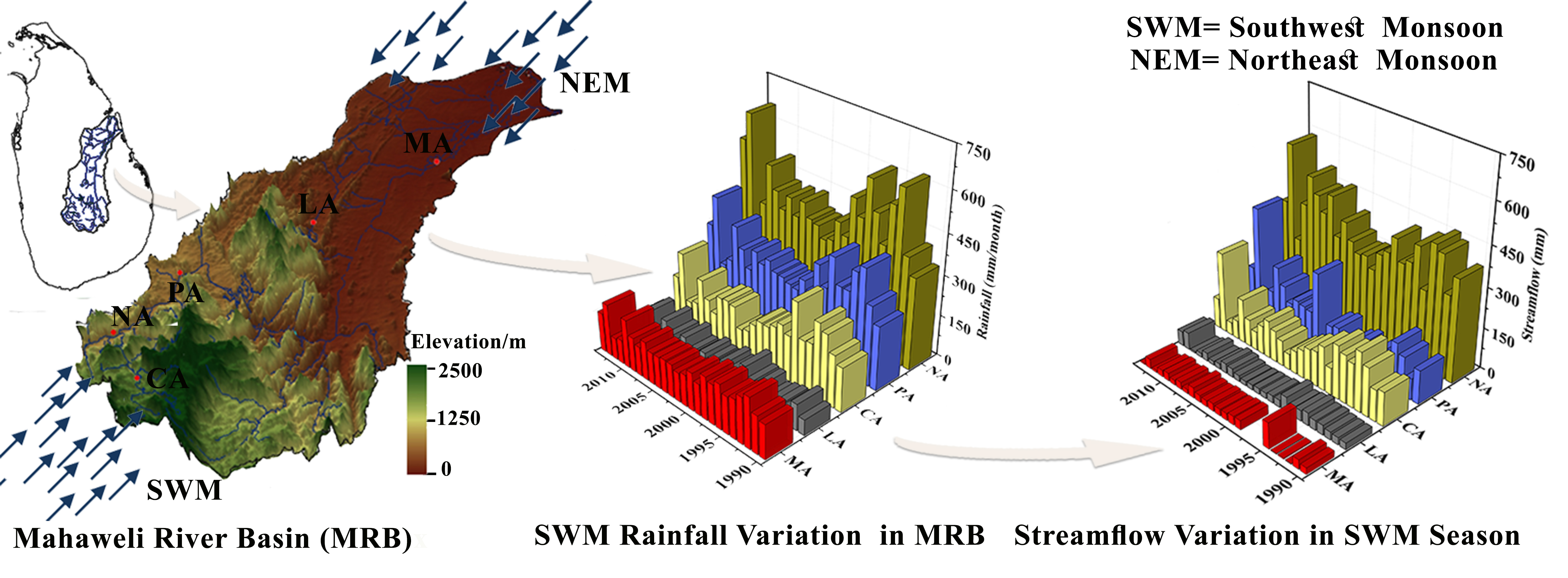
The previously defined boundaries of the UMRB and LMRB [35] are utilized in this study to demarcate two reaches of the river basin. The associated watersheds in six river gauging stations are delineated using the SRTM digital elevation model (Figure 1b). After delineated catchments based on the river gauges, three catchments (Calidoniya-CA, Nawalapitiya-NA, and Peradeniya-PA) are belonging to the upper reaches of MRB (UMRB, 2917.3 km2). There are three catchments, i.e., Laggala (LA), Thaldana (TH), and Manampitiya (MA), located in lower reaches of the MRB (LMRB, 7345.7 km2). Figure 1c shows elevation profile along the main channel of the Mahaweli River. The topography range for CA, NA, and PA catchments are 1327–2060 m, 562–1300 m, and 467–2060 m, respectively. The topography range of LA, TH, and MA catchments are 163–1657 m, 300–1337 m, and 39–2264 m, respectively. As shown in Table 1, the area of CA, NA, PA, and LA catchments are 185.1, 143.7, 1146, and 117.9 km2, respectively. The MA catchment (5929 km2) has comprised the UMRB (2917.3 km2) and part of the LMRB (3011.7 km2). The streamflow in NA and CA catchments in the UMRB and also streamflow at LA and TH catchments in the LMRB are less influenced by human activities such as reservoir operations and water diversion for irrigation. However, the streamflow in PA catchment can be influenced by the reservoir operation for hydropower generation to some extent, and the river diversion can also modulate the streamflow of MA catchment at Pollgolla barrage.
The daily streamflow data recorded in outlets of six catchments over the MRB are obtained from the Department of Irrigation, Sri Lanka, from 1990 to 2014. The spatial distribution of river gauging stations and their characteristics are presented in Figure 1a and Table 1, respectively. Three river gage stations (Nawalapitiya, Peradeniya, and Manampitiya) are located in the main channel of Mahaweli river while Claidoniya, Thaldana, and Laggala river gauges are located in the branches of Mahaweli river are called as Agra Oya, Badulu Oya, and Kalu Gaga, respectively. Thaldana catchment in the LMRB is not used for analysis due to the lack of long-term daily streamflow records. The daily precipitation records from 43 rain gauge stations covering the MRB are provided by the Department of Meteorology, Sri Lanka, for the period of 1990–2014. The SRTM digital elevation model (30 m resolution) is downloaded from the global topography database (http://earthexplorer.usgs.gov/). The present study used 1° × 1° resolution Sea surface temperature (SST) data from the Met Office Hadley Center Sea Ice and Sea Surface Temperature version 1.1 (HadISST1.1) [36] to calculate the Niño3.4 index, which represents the central tropical Pacific ocean conditions. Besides, the Dipole mode index (DMI) has been calculated, which denotes the east-west temperature gradient across the tropical Indian Ocean [37] using the same SST data product.
2.2. Methodology
It’s well known that there are four seasons on Sri Lanka and other South Asian countries, which are defined by the rainfall and circulation patterns over the country, i.e., southwest monsoon (SWM; June–September), northeast monsoon (NEM; December–February), first inter-monsoon (FIM; March-May) and second inter-monsoon (SIM; October–November), respectively [38,39]. The area average annual and seasonal rainfall in delineated catchments, i.e., CA, NA, PA, LA, and MA, are calculated for the period 1990–2014 to investigate the seasonal cycle of streamflow and rainfall and their relationship over MRB. For estimating area average rainfall, the Thiessen polygon (TP) method is widely used in hydrology and meteorology [40,41]. However, the simplistic TP method is suitable for estimating monthly precipitation in the flat terrains [42]. The rainfall amount in the mountainous watershed is also dependent on the local topography. Therefore, the area average rainfall is calculated by combining the TP method with the elevation regression method [42], and this method has been applied to calculate the area average rainfall in mountainous catchment [43]. In this study, the rain gauges data inside the delineated catchment boundary are used to calculate area average precipitation using the above-mentioned method. As there is no rain gauge inside the LA catchment (Table 2), the nearest two rain gauges outside the LA catchment (with distance of 2.6 km and 6.8 km, respectively) are used to calculate the area average rainfall in LA catchment. Noting that the combined method is not applied to calculate the area average rainfall in CA and LA catchments due to the less number of stations (<3). For demonstrating the spatial distribution of seasonal rainfall over MRB, the Cressman interpolation technique [44] is adopted to interpolate the rain gauge data into 0.1 × 0.1 degree grid-cell data.
As an initial stage of analysis, daily streamflow time series with more than 15% missing values within the analysis period are excluded in calculating the monthly average. If there is a one- or two-day gap in the daily dataset, the missing values are interpolated by calculating the average of proceeding and succeeding two days daily streamflow. The low, medium, and high streamflow are widely used as hydrological indicators in water research and management [18]. In this paper, seasonal streamflow characteristics will also be computed and analyzed for the above mentioned four different seasons. In addition, the 5th, 50th, and 95th percentiles of daily streamflow for the different seasons (SWM, NEM, FIM, and SIM) have been calculated for each catchment. The low flow (Q5), median flow (Q50), and high flow (Q95) are related to the 5th, 50th, and 95th percentile value of the daily streamflow, respectively. The Max10-day flow and Max30-day flow, prevalence of flows below Q5 (PQ5), and prevalence flow above Q95 (PQ95) [18,21] are considered as indices to identify the extreme streamflow events. To understand the variability of streamflow extremes, time series of Max10-day flow, Max30-day flow, PQ5, and PQ95 are analyzed. The top 10 and 30 maximum daily streamflow records for the given season in each year are selected to calculate the average of Max10-day and Max30-days flow (m3 s−1), respectively. To calculate the PQ5 in each catchment for different seasons, the numbers of days, which are below the Q5 values, are counted. Similarly, the numbers of days that exceed the Q95 are counted to get PQ95.
3. Result and Discussion
3.1. Seasonal Cycle of Rainfall and Streamflow
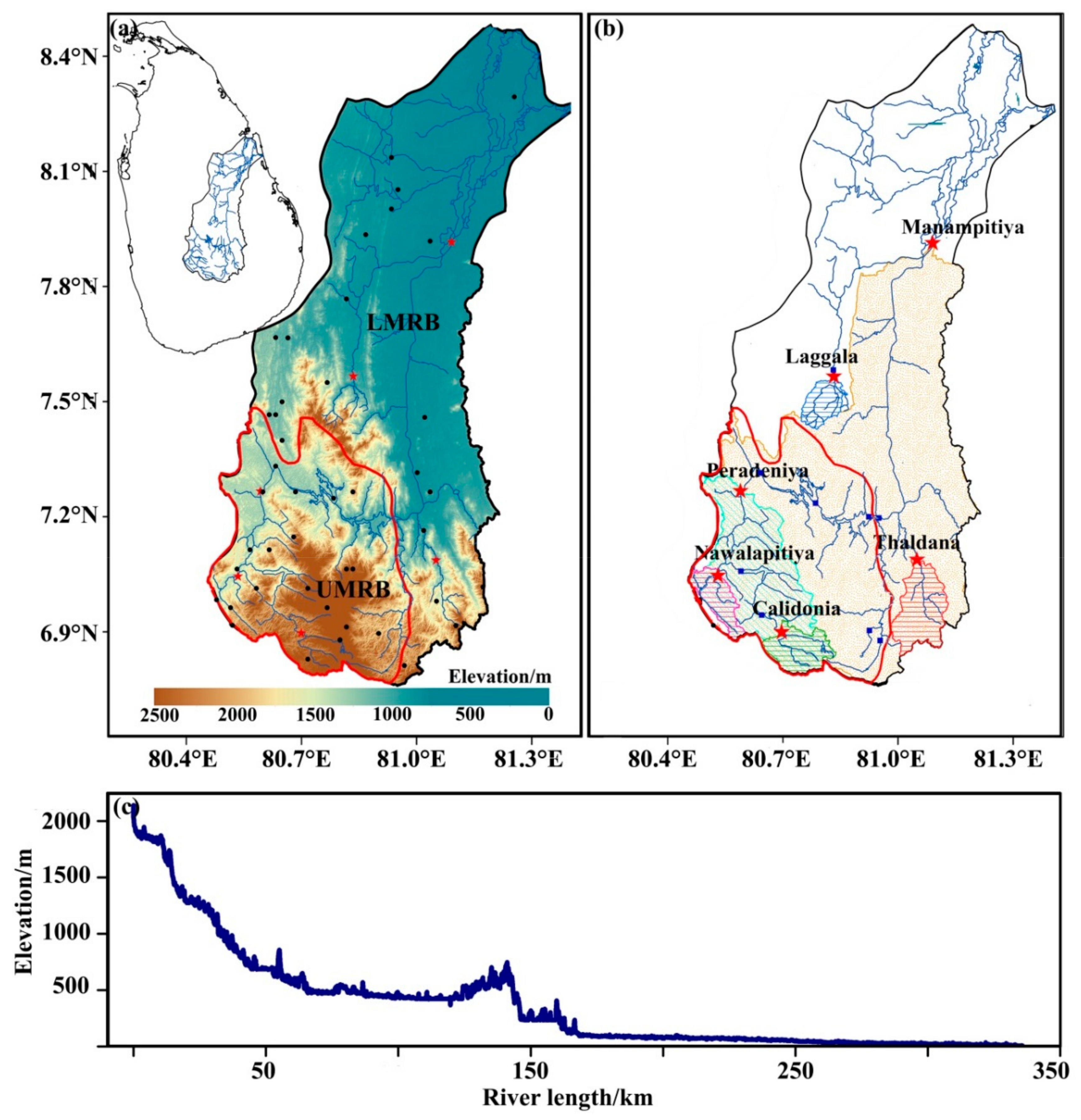
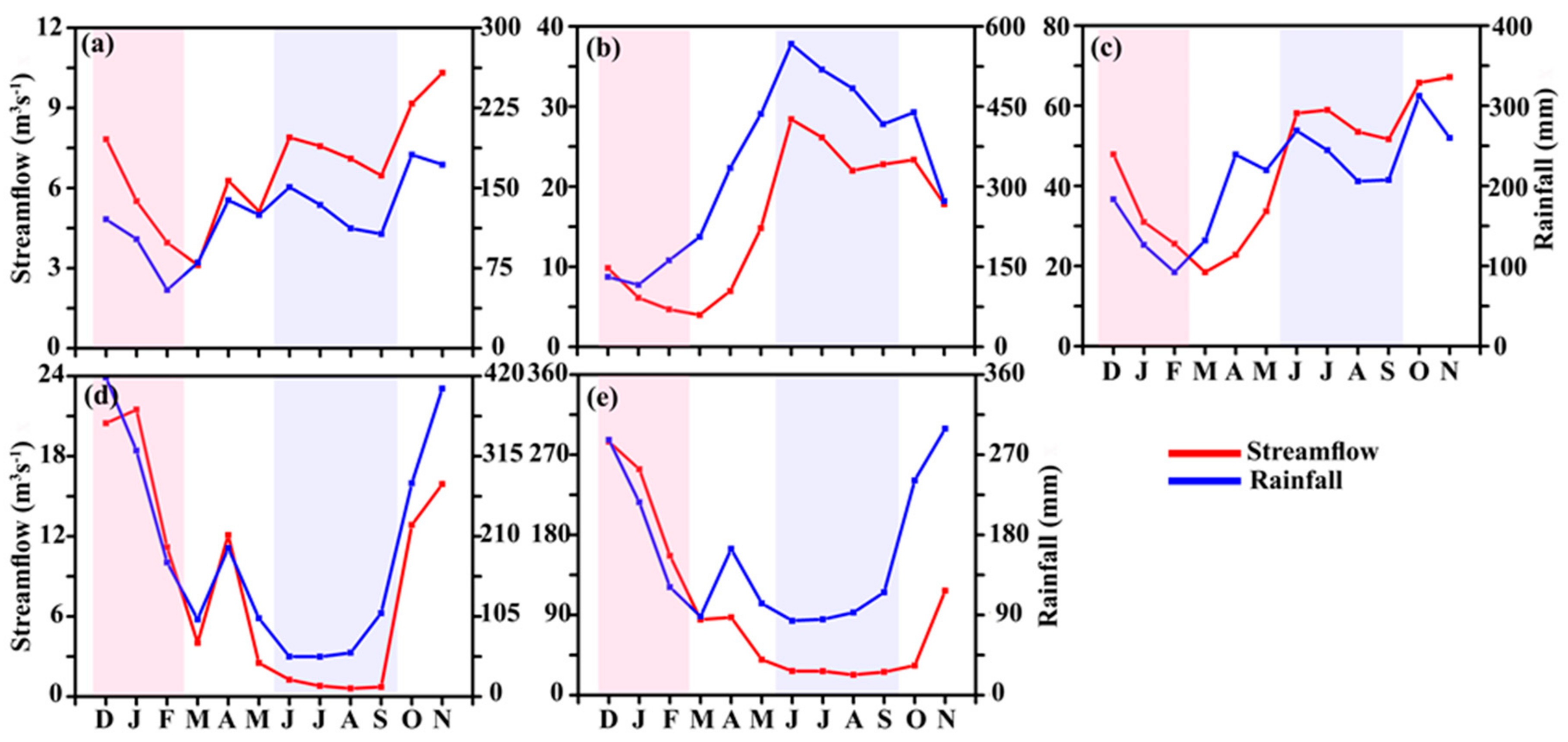
Figure 2 shows the seasonal cycle of mean monthly streamflow and rainfall in CA, NA, PA, LA, and MA catchments of the MRB for the period 1990–2014. The close association between the annual cycle of streamflow and rainfall over catchments in the UMRB and LMRB can be found. For the UMRB, two dominant peaks of rainfall (June and October) are observed in the CA, NA, and PA catchments (Figure 2a–c). During the SWM season (June to September), the maximum rainfall is recorded in June with relatively less rainfall observed during August and September in the UMRB. The lowest rainfall and streamflow of the CA, NA and PA catchments are recorded from December to February (Figure 2a–c), which are responding to the cease of the NEM season.
The LA and MA catchments in the LMRB have recorded more rainfall and streamflow from November and January. According to Figure 2d–e, the lowest streamflow of the LA and MA catchments are observed from May to September, and less rainfall can be found from February to September, except that there are small peaks in April both for rainfall and streamflow. Based on the station data analysis, we can find that the streamflow of each catchment is closely associated with rainfall variation over both the upper and lower reaches of the MRB. For the long-term average (1990–2014) of rainfall in MRB, annual total rainfall of the LMRB and UMRB are estimated to be 1823 and 2158 mm, respectively. Out of these, the LMRB received the highest seasonal rainfall during the NEM season, which is about 41.0% of the annual total. In addition, the LMRB received 30.5%, 16.9%, and 11.6% rainfall during the SIM, FIM, and SWM seasons, respectively. The UMRB recorded more than 50% of the total rainfall during the SWM (29.7%) and SIM (25.9%) seasons. On the other hand, the contributions of the NEM and FIM rainfall to annual total rainfall of the UMRB are 24.3% and 20.1%, respectively.
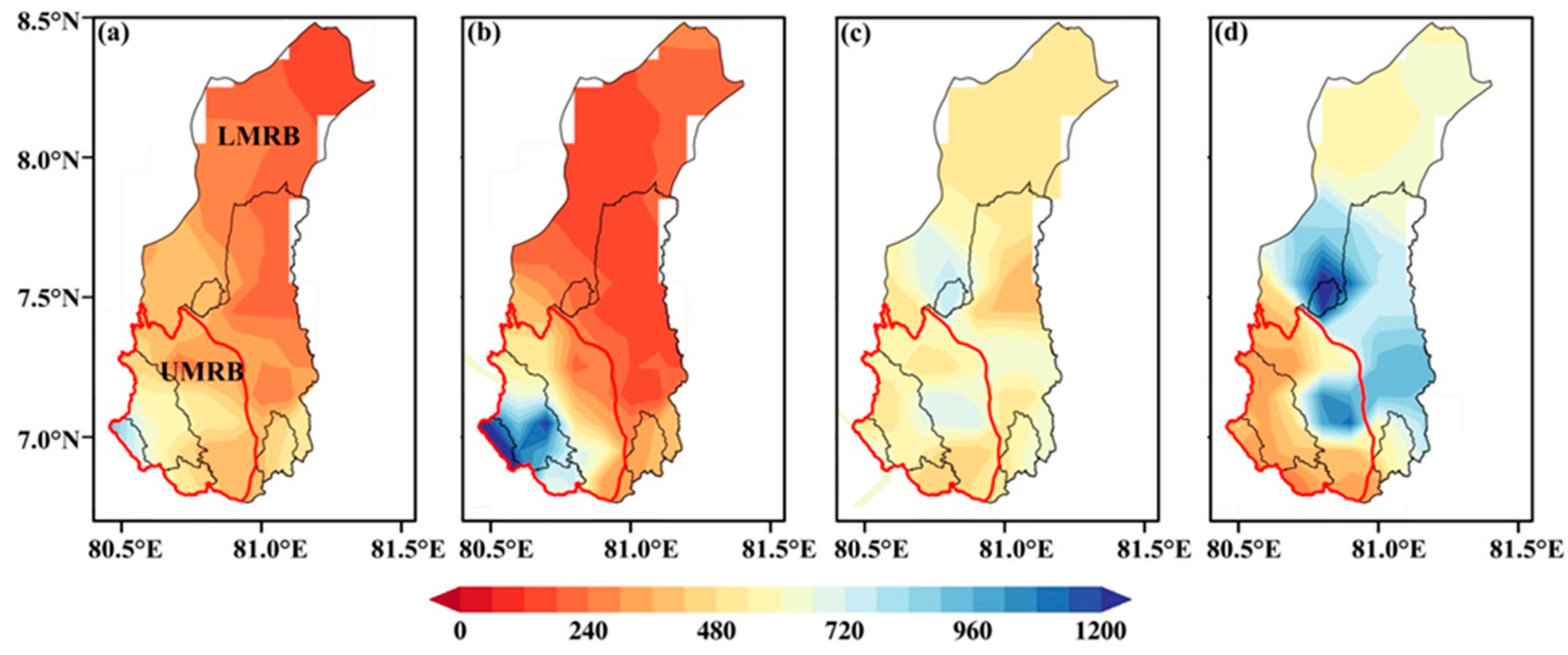
The total rainfall distribution in each season over the MRB during the period of 1990–2014 is displayed in Figure 3. In addition, Table 2 provides the rainfall variation in selected catchments for different seasons. During the FIM season, the total rainfall is higher in the southwestern part of the catchment (NA, 924 mm) than rest of the MRB catchments (Figure 3a), while most of the area received less than 350 mm rainfall in total (Table 2). Due to the orographic rainfall on the windward side of the mountain ridge, the western and southern parts of the MRB receive more rainfall during the SWM season (Figure 3b). The maximum and minimum rainfall during the SWM season is recorded in NA (1987 mm) and LA (271 mm) catchments, respectively.
Figure 3c represents total rainfall distribution in the SIM season. In general, the whole basin receives more than 500 mm in total rainfall during the SIM season, regardless of the orographic influence of central mountains in Sri Lanka. In the SIM season, the NA (712 mm) catchment recorded maximum rainfall, while the lowest rainfall is observed in the CA (353 mm) catchment (Table 2). According to Figure 3d, the total amount of rainfall from the NEM season in the LMRB and eastern part of the UMRB is higher than rainfall received in the western and southern parts of the UMRB. During the NEM season, the LA catchment recorded the highest rainfall (923 mm), and the CA catchment receives the lowest rainfall (277 mm).
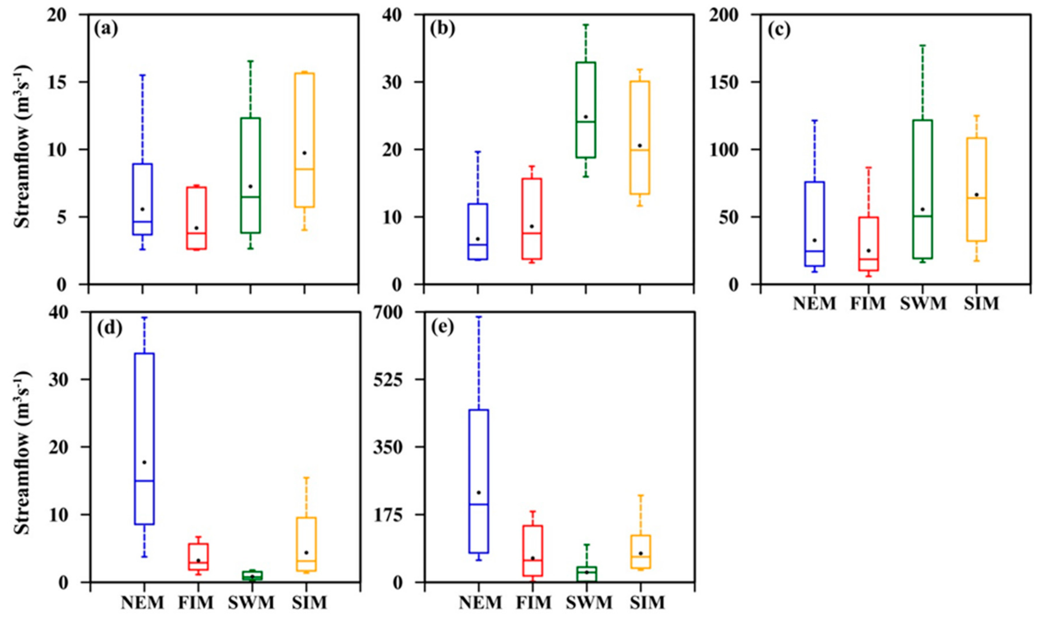
The seasonality of streamflow differs extensively among the basins and is influenced mostly by the local seasonal cycle of precipitation [45]. To identify the seasonality of Mahaweli streamflow, the median, mean, minimum, and maximum, streamflow in each catchment for the four seasons are analyzed (Figure 4). In addition, the 10th and 90th percentile of the seasonal streamflow are displayed by the lower and upper boundary of the box. For the UMRB, CA (9.73 m3 s−1) and PA (66.43 m3 s−1) catchments recorded the larger mean monthly streamflow during the SIM season than the other three seasons (Figure 4a,c). The NA (28.2 m3 s−1) catchment recorded the highest average monthly streamflow during the SWM season (Figure 4b). The mean streamflow of the LA (17.1 m3 s−1) and MA (231.8 m3 s−1) catchments during the NEM season are higher than the other three seasons. Lowest monthly mean streamflow in the LA (0.85 m3 s−1) and MA (22.08 m3 s−1) catchments have been observed in the SWM season (Figure 4d–e).
The large variation between maximum and minimum streamflow is also observed in the SWM season for the UMRB catchments. The difference between minimum (2.6 m3 s−1) and maximum (16.2 m3 s−1) streamflow in the CA catchment during the SWM season is larger than other seasons. For the NA (PA) catchment, the minimum and maximum streamflows are 15.5 (16.4) and 38.4 (180.0) m3 s−1, respectively, which observed during the SWM season. In the same season, both catchments exhibit larger variation of streamflow as compare to other seasons. The LA catchment depicts large variation between maximum (39.1 m3 s−1) and minimum (3.7 m3 s−1) streamflow during the NEM season. Similarly, the MA catchment recorded a large difference between minimum (57.0 m3 s−1) and maximum (687.3 m3 s−1) streamflow during the NEM season compared to other seasons.
The CA catchment recorded the highest 95th percentile streamflow (15.8 m3 s−1) during the SIM season. The NA (32.4 m3 s−1) and PA (116.4 m3 s−1) catchments recorded the highest 95th percentile streamflow during the SWM season. The lowest 10th percentile streamflow for the CA (2.6 m3 s−1), NA (3.9 m3 s−1), and PA (10.3 m3 s−1) catchments are recorded in the FIM season. The highest 90th percentile streamflow in the LA and MA catchments is 33.5 and 441.2 m3 s−1, respectively, that recorded in the NEM season. The lowest 10th percentile streamflow for the LA (0.5 m3 s−1) and MA (39.1 m3 s−1) catchments are observed in the SWM season.
As extreme streamflow indicators, the average Max10-day flow and Max30-day flow for the FIM, SIM, SWM, and NEM seasons are shown in Table 3. The largest average value of Max10-day flow in the CA (21.0 m3 s−1), NA (76.3 m3 s−1), and PA (134.8 m3 s−1) catchments is observed during the SWM season. Compare to the other seasons, the average value of the Max30-day flow also recorded the largest magnitude during the SWM season for catchments in the UMRB. The lowest Max10-day flow and Max30-day flow of the CA and PA catchments are observed in the FIM season. The average Max10-day flow (14.7 m3 s−1) and Max30-day flow (10.9 m3 s−1) events in the NA catchment are lowest, which is recorded during the NEM season. As compared to the maximum value in a different season, the average Max10-day flow (70.0 m3 s−1) and Max30-day flow (38.4 m3 s−1) at LA catchment in the LMRB are observed during the NEM season. For MA catchment, the largest average value of Max10-day flow (Max30-day flow) is 759.1 m3 s−1 (466.7 m3 s−1), which is recorded in the NEM season. The lowest Max10-day flow and Max30- day flow at both catchments in the LMRB are recorded during the SWM season (Table 2). The results clearly show that the high streamflow extremes in the UMRB catchments are mostly found in the SWM season when heavy and very heavy rainfall occurs frequently. In the LMRB catchments, extreme high flow events can be found during the NEM season, the rainy season for the catchments. This is consistent with the result by Groisman et al. [46], i.e., the variations of high and very high streamflow are closely associated with heavy and very heavy precipitation.
3.2. Inter-Annual Variation of Streamflow
Understanding of year-to-year variations in streamflow is important for the development and management of water resources in most regions. Considering the contribution of seasonal rainfall to the total annual rainfall, the SWM season for the UMRB and NEM season for the LMRB are important than the other two inter-monsoonal periods. Meanwhile, maximum streamflow in the UMRB (LMRB) catchments is recorded during the SWM (NEM) season, while the minimum streamflow in the UMRB (LMRB) catchments is observed during the NEM (SWM) season. Therefore, the SWM and NEM seasons are selected in this study.
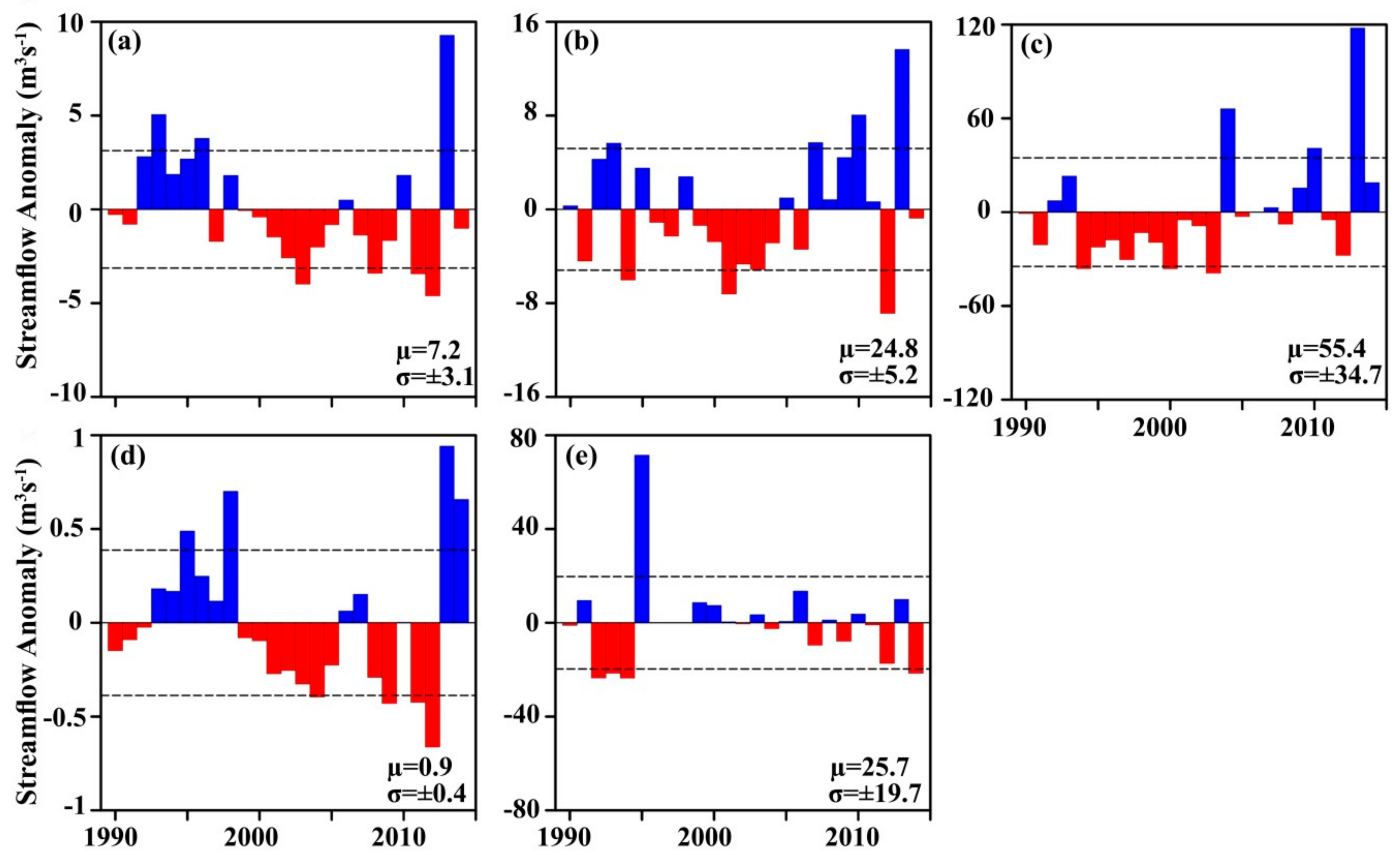
The anomalous streamflow variation of each catchment during the SWM season is depicted in Figure 5. For the UMRB, where rainfall is significantly influenced by the SWM, different features for the interannual variation of seasonally averaged streamflow can be found for different sub-basins. The streamflow of CA catchment indicates a positive anomaly from 1992 to 1996, with streamflow anomalies in 1993, 1996, and 2013 exceeding one standard deviation (σ). Generally, it is noticed that most of the years after 1997 inherited a negative anomaly of streamflow except 1998, 2006, 2010, and 2013 (Figure 5a). The streamflow of the NA catchment shows a negative anomaly from 1991 to 2006 except 1992, 1993, 1995, 1998, and 2005. Among negative anomalies, streamflow anomaly in 1994, 2001, 2003, and 2014 are below the −1σ (5.2 m3 s−1) level. Positive streamflow anomalies can also be found from the 2007–2013 period, except 2012. Furthermore, streamflow anomalies in 2007, 2010, and 2013 can exceed the +1σ level (Figure 5b).
In the PA catchment, streamflow during the SWM season shows a negative anomaly for most years from 1990 to 2008, except for 1992, 1993, 2004, and 2007 (Figure 5c), with the magnitude of anomalies below −1σ (34.7 m3 s−1) level. Based on all catchments in the UMRB, the year 2013 shows a remarkable positive anomaly of streamflow. The streamflow of the LA catchment shows a negative anomaly from 1999 to 2012 except 2006, 2007, and 2010, and 2009, 2011, and 2012 recorded negative anomaly below the −1σ (0.4 m3 s−1). Considering the interannual variation of streamflow anomaly in the LA catchment during the SWM season, the positive streamflow anomalies can be found from 1993 to 1998, and for 2013 and 2014, with large than +1σ (0.4 m3 s−1) positive streamflow anomaly found in 1995, 1998, 2013 and 2014 respectively (Figure 5d). The MA catchment indicates a negative anomaly of streamflow below the −1σ (19.7 m3 s−1) level in 1992, 1993, 1994, and 2014, while the positive anomalies exceeding the +1σ level are recorded only in 1995 (Figure 5e).
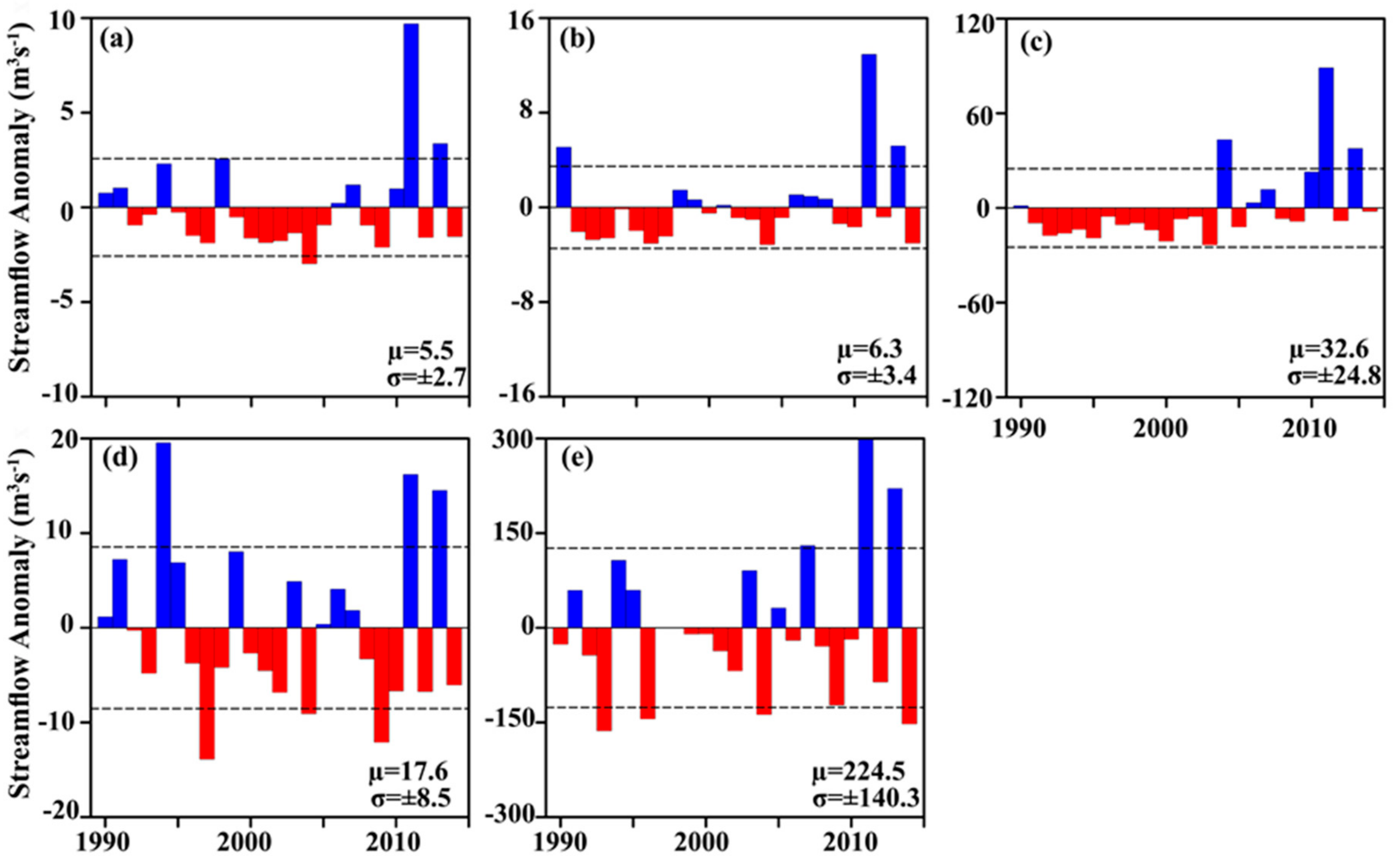
Figure 6 shows the anomalous streamflow at five catchments in the MRB during the NEM season. The magnitude of streamflow anomalies of the UMRB catchments during the NEM season is smaller compared to that during the SWM season (Figure 6a–c). The contrast pattern is observed for the LA and MA catchments (Figure 6d–e). The CA catchment showed the largest positive streamflow anomaly (5.5 m3 s−1) in 2011, followed by 2013, while the year 2004 indicates a negative streamflow anomaly, which is below −1σ (2.7 m3 s−1) level. For the NA catchment, larger than +1σ (3.4 m3 s−1) positive streamflow anomalies are recorded in 1990, 2011, and 2013. In the PA catchment, the negative anomalies of streamflow are observed from 1990 to 2005 except 2004, while positive anomalies that exceed the +1σ (24.8 m3 s−1) level are recorded in 2004, 2010, and 2013 (Figure 6c). The positive streamflow anomaly of streamflow of the LA catchment exceeds +1σ (8.5 m3 s−1) in year 1994, 2011 and 2013, while a strong negative anomaly (below –8.5 m3 s−1) recorded in 1997, 2004 and 2009 (Figure 6d). In the MA catchment, 1993, 1996, 2002, 2008, and 2014 exhibit negative anomalies of streamflow, which exceed the −1σ (140.3 m3 s−1) level, while streamflow for the NEM season in 2011 and 2013 show large positive anomalies exceeding +1σ (140.3 m3 s−1) (Figure 6e).
To identify the variability in each catchment, the variance (σ2) has been calculated for the SWM and NEM seasons. The variance of the streamflow in CA, NA, and PA catchments is 10.24 m6 s−2, 27.04 m6 s−2, and 1207.4 m6 s−2, respectively, for the SWM season. In the NEM season, the variance of the CA (7.29 m6 s−2), NA (11.56 m6 s−2), and PA (615.04 m6 s−2) catchments are smaller than that in the SWM season. Based on variance, the strong interannual variation of mean streamflow at CA, NA, and PA catchments in the UMRB is observed during the SWM season. The strong interannual variation of streamflow during the NEM season is recorded in the LA (72.5 m6 s−2) and MA (19,600 m6 s−2) catchments (Figure 6d–e) compared to the SWM season. As shown in the annual cycle of the rainfall over each catchment (Figure 2), rainfall also showed peaks during the SWM and NEM seasons in the UMRB and LMRB, respectively.
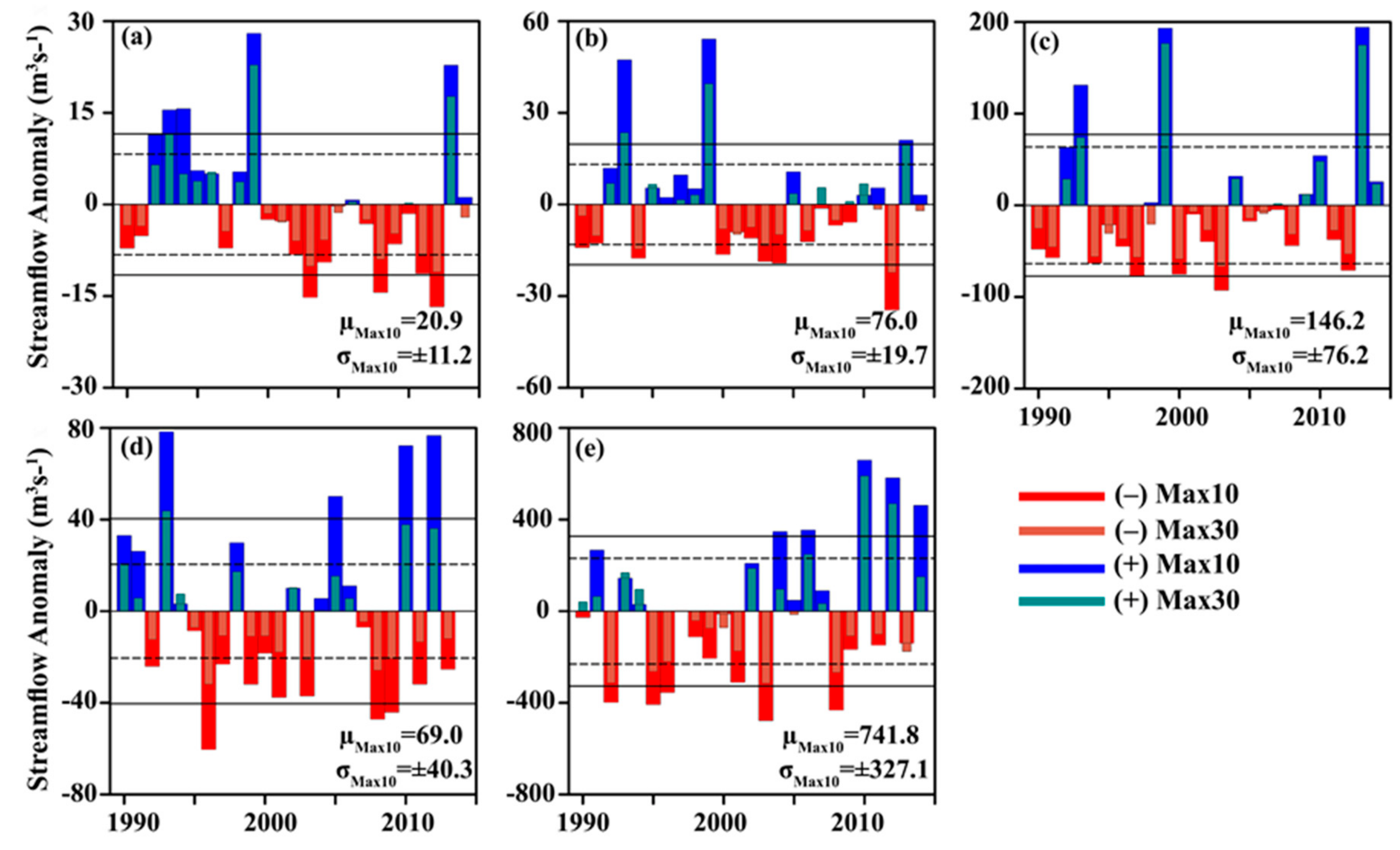
Max10-day flow, Max 30-day flow, PQ5, and PQ95 are selected to analyze the interannual variation of extreme flow events in SWM and NEM season for selected catchments. The variation of Max10-day and Max30-days flows in the CA, NA, and PA catchments during the SWM season are shown in Figure 7a–c. The lower two panels show the interannual variation of the aforementioned extreme flow indices in the LA and MA catchments during the NEM season.
According to the magnitude of an anomaly, Max10-day is larger than Max30-day in each catchment, and the interannual variation of both indices exhibit a similar pattern. In the CA, NA, and PA catchments, the recorded average Max10-day flow (Max30-day flow) are 20.9, 76.0, and 146.2 (14.5, 52.1, and 110) m3 s−1, respectively. In terms of the Max10-day flow and Max30-day flow anomalies of catchments in the UMRB, the year 2003, 2008, 2011 and 2012 showed strong negative anomalies, while 1993, 1999 and 2013 showed positive anomalies (Figure 7a–c). In general, the more negative anomaly of Max10-day and Max30-day flows in the CA catchment is recorded after 2000 except 2013. The same observation is recorded in the NA catchment. The positive anomalies of Max10-days flow in the NA, and PA catchments that exceed the +1σ are observed during the SWM season in 1993, 1999, and 2013 (Figure 7b–c). According to the variation of Max10-day, and Max30-days flow over the study period, catchments in the UMRB recorded more negative anomalies in the SWM season during 1990-2014.
Figure 7d shows the interannual variation of Max10-day and Max30-day flow in the LA catchment during the NEM season. The averaged Max10-day is 69.0 m3 s−1 in the LA catchment, and averaged Max30-day is 38.4 m3 s−1. The anomaly of Max 10-days and Max 30-days flow in the LA catchment exceed the +1σ in 1993, 2005, 2010, and 2012. For 1996, 2008, and 2009, the anomaly of Max10-day and Max30-day flow is below the −1σ (Figure 7d). In the MA catchment, the negative anomaly below the −1σ of Max10-day and Max30-day flow are observed in 1992, 1995, 1996, 2003, and 2008. However, the positive anomalies of these indices in MA catchment are observed in 2004, 2006, 2010, 2012, and 2014 (Figure 7e).
Although there exists strong interannual variability of Max10-day and Max30-day flows at both catchments in the LMRB, the magnitude of the variability is relatively higher after 2005 than that before 2005. This is different from the situation in UMRB, where the interannual variability is relatively larger before 2005. And this could be ascribed to the different changes of interannual variability of SWM and NEM monsoon rainfall.
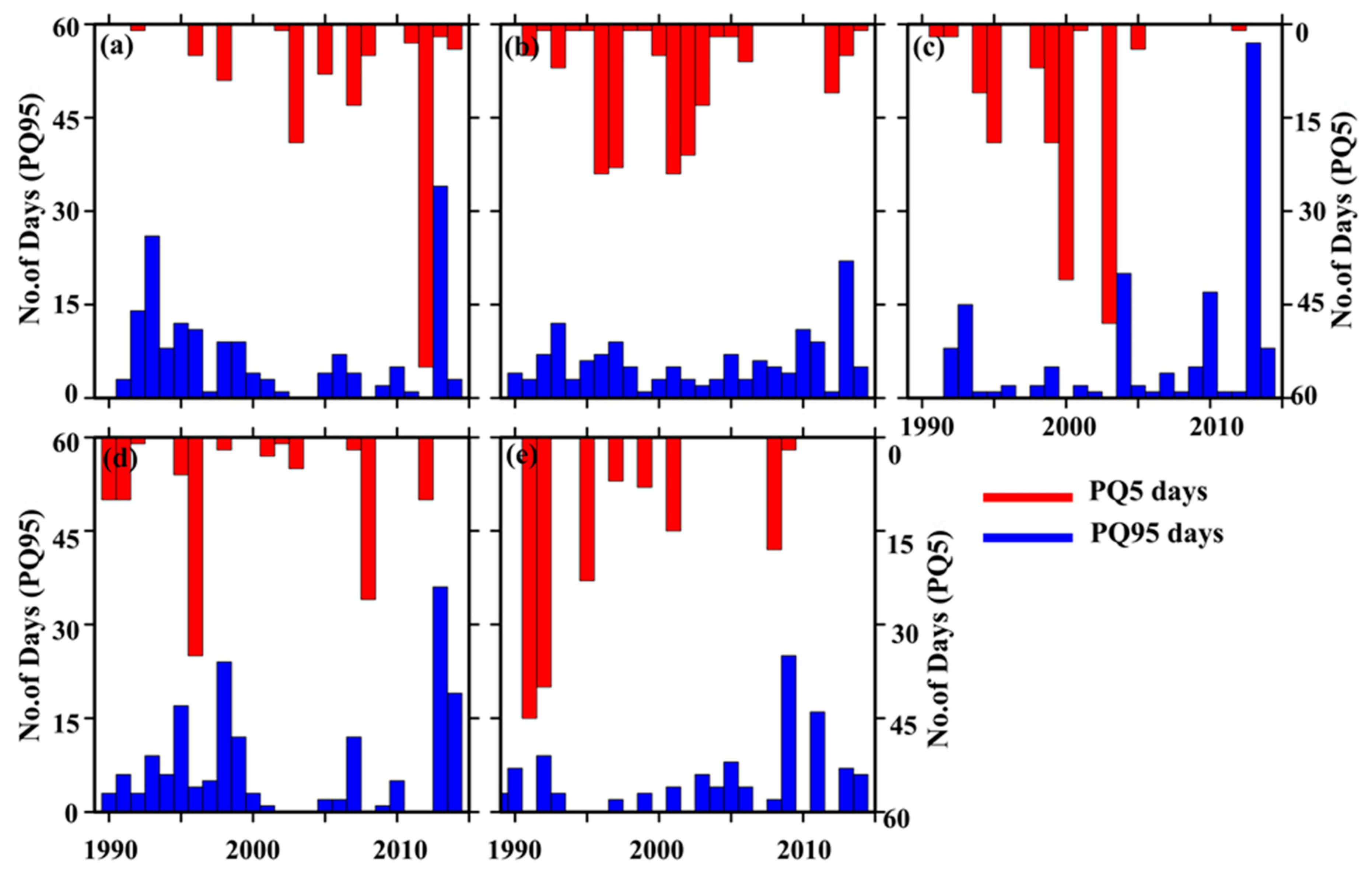
Figure 8a–c shows the interannual variation of the number of low flow days with streamflow below the 5th percentile and high flow days with streamflow larger than the 95th percentile during the SWM season. The lower two panels (Figure 8d–e) are the same as above but for the NEM season. The 5th (95th) percentile flow in the CA, NA, PA, MA, and LA catchments are 2.7 (18.6), 2.1 (65.8), 8.1 (147.3), 10.1 (840.8), and 2.3 (57.3) m3 s−1, respectively. The number of low flow days in the CA catchment is recorded more after 2000, while the number of days recorded high flow events are larger during 1990–2000 than the 2001–2014 periods. It also shows the decadal difference of the PQ5 and PQ95 in the SWM season (Figure 8a). The Q95 flow at NA catchment recorded less than 15 days during the every SWM season. The PQ5 events in the NA catchment are higher during 1990–2005 (Figure 8b) compared to the 2006–2014 period. In the PA catchment, PQ5 during the SWM season is higher in 1990–2005, while the maximum number of high flow days above the Q95 flow threshold in SWM season is observed in 2013 (57 days), followed by 2004 (20 days) and 2010 (17 days) (Figure 8c).
For the NEM season, the prevalence flow above Q95 in the LA catchment shows more events during the 1990–2000. In the year 2013, it recorded the maximum number of days (36 days). The recorded low flow events in the LA catchment during the NEM season are comparatively less in 2000–2014 except for 2008 and 2012 (Figure 8d). Figure 8e shows the prevalence flow of Q5 and Q95 in the MA catchment for the NEM season. In the MA catchment, 45 and 40 days in the year 1991 and 1992 are the recorded number of days, which are below the Q5 percentile flow event. However, most of the years after 2000 have zero-days, which recorded Q5 percentile flow events, except 2008 and 2009.
3.3. The Relationship Between Rainfall and Streamflow
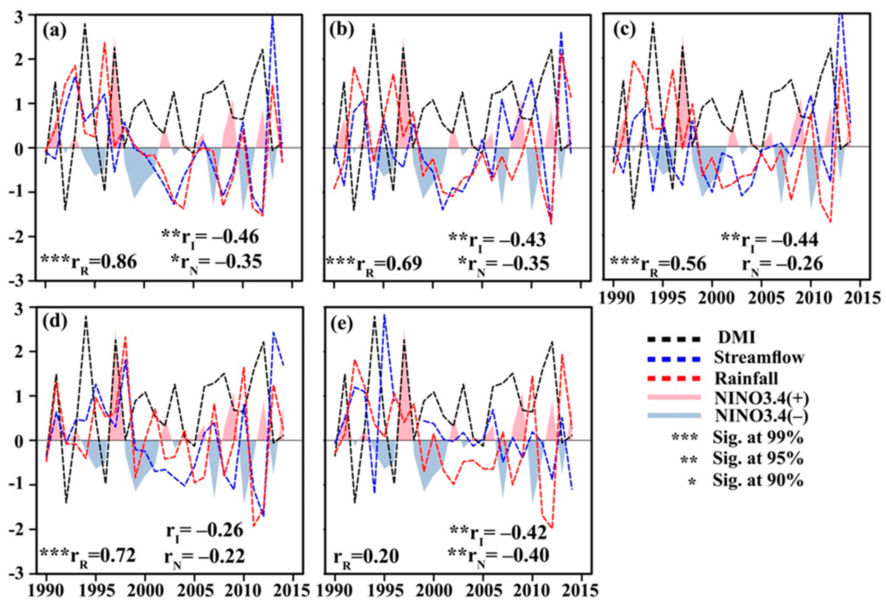
Numerous studies in many different countries have conclusively shown that rainfall changes affect the streamflow [10,47]. In Figure 9, we take a closer look at the correlation between standardized rainfall and streamflow (Q50) in MRB catchments for the SWM and NEM seasons separately (Figure 9 and Figure 10).
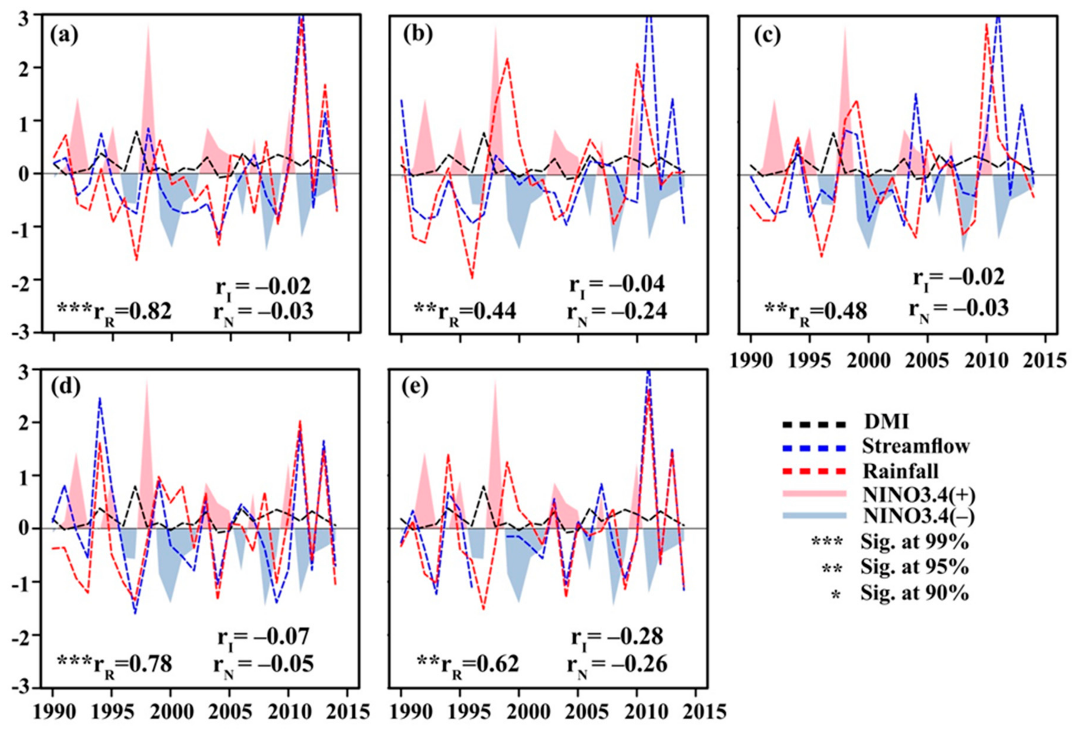
The statistically significant positive correlation between rainfall and Q50 in the CA (0.86), NA (0.69), and PA (0.56) catchments are observed for the SWM season (Figure 9a–c). Considering the LMRB, LA catchment (0.72) recorded a statistically significant positive correlation between rainfall and streamflow for the SWM season (Figure 9d). However, the corresponding correlation is not statistically significant for the MA (0.20) catchment (Figure 9e). For the NEM season, the correlation coefficient of Q50 and rainfall at the CA, NA, and PA catchments in the UMRB are 0.82, 0.44, and 0.48, respectively, while the LA (0.78) and MA (0.62) catchments recorded statistically significant correlation between streamflow and rainfall (Figure 10a–e).
It is interesting to notice that the relationship between rainfall and streamflow in the UMRB during the SWM season is stronger compared to that in the NEM season. However, at the LA and MA catchments in LMRB, the rainfall and streamflow relationship is stronger during the NEM season than in the SWM season.
Abghari et al. [48] found that strong relationships between river discharge and annual precipitation in Iran during the past 40 years. Abeysingha et al. [49] revealed that the significant positive correlation between streamflow and catchment rainfall in the Gomti River basin. When considering the correlation coefficient and year to year variation, it can also be concluded that the rainfall over catchment is the major influencing factor for the streamflow variation in the MRB.
However, the correlation between seasonal rainfall and streamflow in the PA catchment is relatively smaller compared to those catchments in the upper reaches of the Mahaweli basin. Previous studies have suggested that the precipitation–runoff relationship could be modulated by human activities, such as the construction of reservoirs [50] and the hydromechanics project [51]. So the relatively weak rainfall-streamflow correlation could be ascribed to the effects of the construction and operation of the Kothmale (1979–1985) and Upper Kothmale reservoirs in the MRB, which can affect the streamflow in PA catchment. The weak relationship between streamflow and rainfall in the MA catchment is also observed, especially during the SWM season. The main factors, which contribute to show a weak correlation between rainfall and streamflow in the MA catchment, could be the river diversion project for irrigation purpose and reservoirs operation of Mahaweli hydropower complexes.
3.4. Streamflow Response to ENSO and Indian Ocean Dipole
It is noticed that the climate of several countries located in the Indian Ocean, as well as the entire globe, is modulated by the El Niño-Southern Oscillation (ENSO) and Indian Ocean Dipole (IOD) [52]. According to Ward et al. [53], ENSO has significant impacts on streamflow and flooding around the world. To understand the relationship between streamflow and the large scale circulation indices, the concurrent correlation coefficient has been evaluated using the Nino3.4 and DMI indices with streamflow in the SWM and NEM seasons separately.
Figure 9 shows the relationship between streamflow in each catchment and the large-scale SST anomaly signal in the tropical Pacific Ocean (Nino3.4) and the Indian Ocean (DMI) during for the SWM season. The statistically significant negative correlation can be found between the Nino3.4 and streamflow in the CA (–0.35), NA (–0.35), and MA (0.4) catchments for the SWM season. However, the correlation between Nino3.4 Index and streamflow is weak in the PA (–0.26) and LA (–0.22) catchments (Figure 9c,d). The positive mode of the Nino3.4 (El Niño) shows a negative influence on streamflow in MRB, while the contrast response of streamflow in MRB for the negative Nino3.4 (LaNiña) is observed. Similar to our findings, the previous study suggested that the relationship between ENSO indices and Mahaweli streamflow was quite significant from January to September [33] between 1954 and 1993, and El Niño (LaNiña) conditions are also closely associated with annual rainfall and streamflow for January to September in Kelani River basin in Sri Lanka [27]. Furthermore, Ouyang et al. [54] also pointed out that the streamflow during the LaNiña events in different river basins in China was higher compared to the El Niño event. In contrast, the total water flow of the Cauvery river basin in India was lower in the La Niña years than El Niño years as a result of the amount of rainfall received during the La Niña years was lower than rainfall in normal years [55].
A strong negative relationship between the DMI and streamflow in the CA (−0.48), NA (−0.43), MA (−0.44), and NA (−0.48) catchments during the SWM season are observed except streamflow in the LA (−0.26) catchment (Figure 9a–e). It revealed that a positive mode of the DMI shows a negative influence on streamflow in the MRB. For the SWM season, the strong relationship between the DMI and streamflow in the MRB has been observed as compared to the Nino3.4. In contrast, Sahu et al. [56] found a positive correlation (0.36) between the DMI and Citarum River in Indonesia.
As shown in Figure 10, the correlation between the Nino3.4 index and streamflow in each catchment for the NEM season indicates a weak negative correlation. Similarly, the relationship between streamflow and the DMI recorded a negative correlation. Furthermore, it’s found that the influence of the DMI and Nino3.4 on streamflow in MRB is stronger in the SWM season than in the NEM season. Moreover, the influence of the ENSO on streamflow in UMRB catchments during the SWM season is relatively dominant than the influence on streamflow in the LMRB catchments. The predominance of the observed significant correlation suggests that the phase and magnitude of the ENSO and DMI indices could be one of the factors of the streamflow variability in the Mahaweli River basin during the SWM season.
3.5. Influence of ENSO and DMI on Rainfall in MRB
The UMRB received more rainfall during the SWM season, which contributes to the enhanced streamflow in the Mahaweli River. However, the dry zone in Sri Lanka, including the Mahaweli development zones (MDZ), exhibits severe water shortage as a result of less rainfall over the area during the same monsoon period, so the Mahaweli water resource is diverted at Pollgolla barrage to overcome the water scarcity in the dry zone and MDZ. So it’s very important to understand the influence of SST anomalies on the SWM rainfall pattern in the Mahaweli river basin, in order for better water resource management. Therefore, the correlation between SWM rainfall in the UMRB and LMRB and SST is analyzed in this section. During the NEM season, the LMRB receives 41% total rainfall. Therefore, recognizing the relationship between two ocean indices is also beneficial to the NEM rainfall prediction and water resource management.
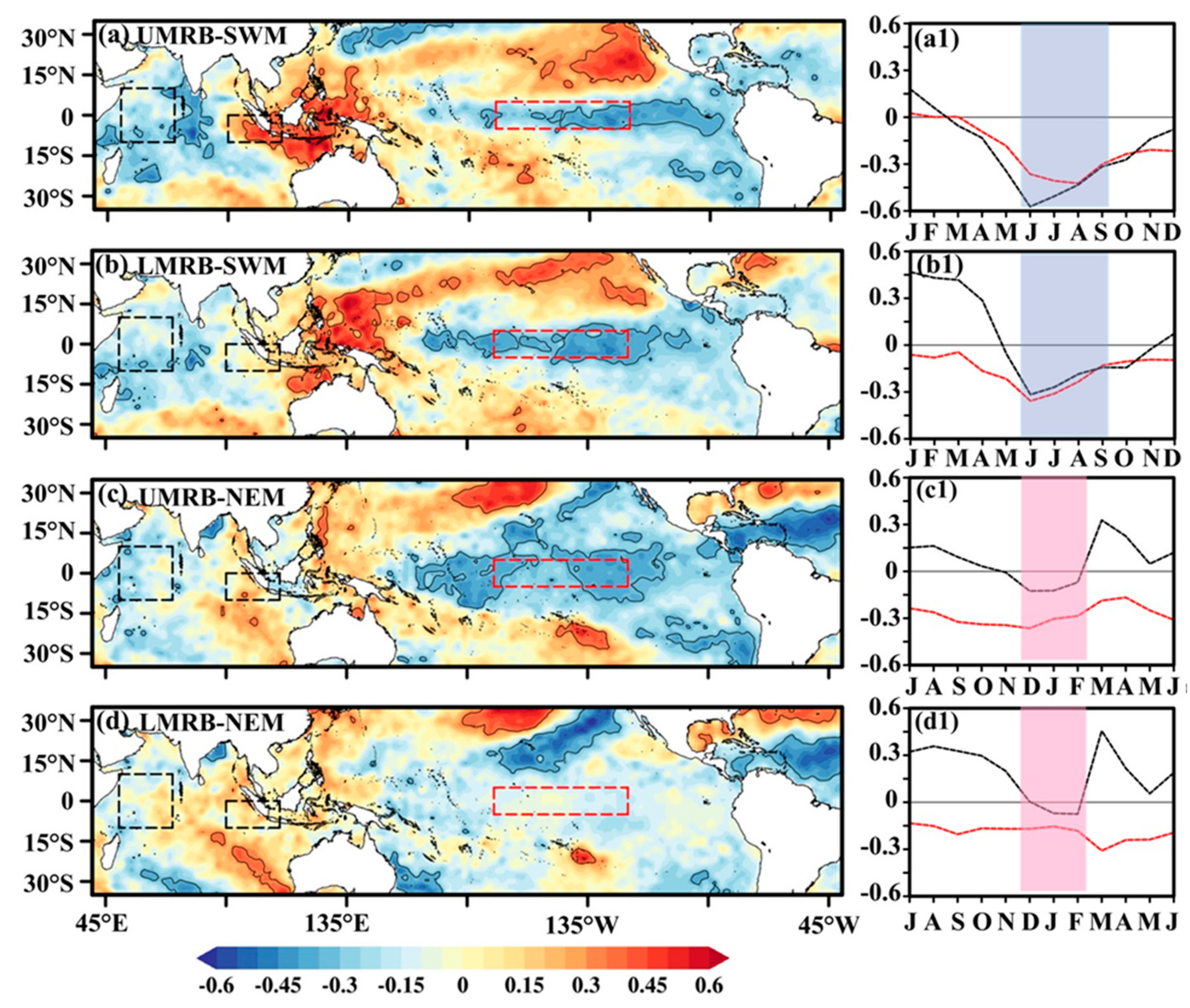
Figure 11a shows the correlation of the SWM rainfall anomaly in the UMRB with SST anomalies in June, which is the starting month of the SWM over Sri Lanka. The lead-lagged correlation between the SWM rainfall in the UMRB and SST are shown in Figure 11a1. The maximum correlation between the rainfall over the UMRB with Nino3.4 (−0.40) is observed in August. The month of June recorded the maximum correlation (−0.57) with the DMI and the SWM rainfall in the UMRB. Figure 11b is the same as Figure 11a but for the LMRB. The rainfall anomaly in the initial month of the SWM shows a strong correlation (−0.35) with the Nino3.4 index. Similarly, the correlation between the DMI and rainfall anomaly in the LMRB is −0.31. However, the positive correlation with SWM rainfall anomaly and the DMI is observed in lagged 3, 4, and 5 months for the LMRB (Figure 11b1).
The spatial correlation between SST in December (Starting month of NEM) and rainfall anomaly of the NEM in theUMRB is shown in Figure 11c, and associated lead-lagged correlation is displayed in Figure 11c1. The correlation between SST in December with the NEM rainfall in the UMRB is −0.36, which is statistically significant, as shown in Figure 11c1. However, the DMI showed weak correlation (–0.12) with the NEM rainfall anomaly in the UMRB for December. Figure 11d shows the correlation between SST and NEM rainfall over the LMRB. In the LMRB, the correlation between Nino3.4 (DMI) and December rainfall is −0.16 (−0.03) while observed maximum correlation (0.45) with the DMI is recorded in the lead month of March (Figure 11d1). Considering the line graphs, the negative relationships between rainfall anomalies in two monsoon seasons and the DMI are found. However, the DMI in lagged and lead months depict a positive correlation with monsoon rainfall anomaly except for the SWM season in the UMRB. Furthermore, the negative correlation between the Nino3.4 index and rainfall anomaly in both monsoon seasons are noted. Similar to our findings, De Silva M and Hornberger [57] found a negative correlation between rainfall in the Kelani river basin Sri Lanka with the Nino3.4 and DMI indices. Addition, Li et al. [58] revealed that a warm phase of the El Niño-Southern Oscillation (ENSO) and a positive Indian Ocean Dipole (IOD) diminish rainfall over the Indian subcontinent and southern Australia.
4. Conclusions
This study has focused on understanding the streamflow variability in five catchments located in the UMRB and LMRB from 1990 to 2014. To identify the streamflow characteristics, the Q5, Q50, and Q95 have been used. In addition, the Max10-day flow, Max30-day flows, PQ5, and PQ95 indices are used for investigating extreme streamflow events. The results clearly show that the strong association between streamflow and rainfall in each catchment. For example, the SWM (NEM) rainfall has more influence on streamflow in the UMRB (LMRB). The strong interannual variability of streamflow in the UMRB (LMRB) is observed during the SWM (NEM) season. Similarly, the strong interannual variation of hydrological extremes, such as Max10-day Max30-days flow, in the UMRB (LMRB) has been recorded during the SWM (NEM) season. It’s further found that more negative anomaly of Max10-day and Max30-day flows in the SWM season can be found after 2000 in the catchments in the UMRB, and this might suggest more frequent hydrological drought events might occur after 2000.
Based on the correlation analysis, the SST anomalies over the western Pacific warm pool, eastern Pacific Ocean, and the western/southwestern part of the Indian Ocean have been found to exhibit a strong relationship with rainfall and streamflow anomalies in the basin. The close relationship between catchment rainfall and streamflow can also be identified from seasonal to interannual time scale in most MRB catchments. However, it also found that the observed streamflow variability signals over some catchments are not significantly correlated with the rainfall variations, and this could be ascribed to effects from human activities, like reservoir operation in PA catchment, dam construction, and streamflow diversion for irrigation purposes in MA catchment.
Because the Mahaweli water from the UMRB is a key water source for hydropower generation and irrigation of the dry zone in Sri Lanka, the year-to-year variation of MRB rainfall and streamflow, including its decadal changes and long term trends, are all of critical importance for the water management not only over MRB but also over the Mahaweli development zones (MDZ). Hence, the understanding of the seasonal streamflow characteristics and variations in different time scales will definitely provide a scientific basis for effective water management over the MRB and decision making for reservoir operations.
It’s noted that, in addition to precipitation, the streamflow variations and change can also be directly modulated by human activities such as flow diversions and irrigation, etc. Meanwhile, the land-use changes in the river basin can also affect the rainfall and streamflow characteristics in the studied watershed. According to Gebrehiwot et al. [59], these types of LULC changes will increase peak flows during the wet season and decrease low flows during the dry season. However, in this study, the impacts from the above-mentioned human activities on the streamflow variations and extremes have not yet been investigated, due to the lack of human practice information. Therefore, further research will be needed to quantify the direct and indirect influence of human activities, like LULC changes and irrigation practice, on the streamflow variations and changes in the MRB.
Author Contributions
All authors collaborated in the research presented in this publication by making the following contributions: research conceptualization, Z.L. and S.S. methodology, Z.L. and S.S.; formal analysis, Z.L. and S.S.; data curation, Z.L. and S.S.; writing—original draft preparation, S.S.; writing—review and editing, Z.L. and S.S.; supervision, Z.L.
Funding
This study is jointly supported by the National Key Research and Development Program (2016YFC0402702), Chinese Academy of Sciences (CAS) Strategic Priority Research Program (grant XDA20060501), and National Natural Science Foundation of China (41661144032).
Acknowledgments
We are thankful to the Meteorological Department and Department of Irrigation, Sri Lanka for providing weather and streamflow data, respectively. The first author acknowledges the CAS–TWAS President’s Fellowship Program for International Ph.D. student, China–Sri Lanka joint Center for Education and Research (CSL-CER), Industrial Technology Institute–Sri Lanka, and also Buddhi Pushpawela and Kritanai Torsri for their help with the preparation of the manuscript. We also thank the anonymous reviewers for their constructive criticism and helpful comments.
Conflicts of Interest
No potential conflict of interest was reported by the authors.
References
- Tomer, M.D.; Schilling, K.E. A simple approach to distinguish land-use and climate-change effects on watershed hydrology. J. Hydrol. 2009, 376, 24–33. [Google Scholar] [CrossRef]
- Miao, C.; Kong, D.; Wu, J.; Duan, Q. Functional degradation of the water-sediment regulation scheme in the lower Yellow River: Spatial and temporal analyses. Sci. Total Environ. 2016, 551, 16–22. [Google Scholar] [CrossRef]
- Rose, S. Rainfall-runoff trends in the south-eastern USA: 1938–2005. Hydrol. Process. 2009, 23, 1105–1118. [Google Scholar] [CrossRef]
- Nilsson, C.; Reidy, C.A.; Dynesius, M.; Revenga, C. Fragmentation and Flow Regulation of the World‘s Large River Systems. Science 2005, 308, 405–408. [Google Scholar] [CrossRef]
- Costa, M.H.; Botta, A.; Cardille, J.A. Effects of large-scale changes in land cover on the discharge of the Tocantins River, Southeastern Amazonia. J. Hydrol. 2003, 283, 206–217. [Google Scholar] [CrossRef]
- Zeng, R.; Cai, X. Analyzing Streamflow Changes: Irrigation-Enhanced Interaction between Aquifer and Streamflow in the Republican River Basin. Hydrol. Earth Syst. Sci. 2014, 18, 493–502. [Google Scholar] [CrossRef]
- Yang, Z.; Liu, Q. Response of Streamflow to Climate Changes in the Yellow River Basin, China. J. Hydrometeorol. 2011, 12, 1113–1126. [Google Scholar] [CrossRef]
- Anil, A.P.; Ramesh, H. Analysis of climate trend and effect of land use land cover change on Harangi streamflow, South India: A case study. Sustain. Water Resour. Manag. 2017, 3, 257–267. [Google Scholar] [CrossRef]
- Pascolini-Campbell, M.A.; Seager, R.; Gutzler, D.S.; Cook, B.I.; Griffin, D. Causes of interannual to decadal variability of Gila River streamflow over the past century. J. Hydrol. Reg. Stud. 2015, 3, 494–508. [Google Scholar] [CrossRef]
- Panda, D.K.; Kumar, A.; Ghosh, S.; Mohanty, R.K. Streamflow trends in the Mahanadi River basin (India): Linkages to tropical climate variability. J. Hydrol. 2013, 495, 135–149. [Google Scholar] [CrossRef]
- Sidibe, M.; Dieppois, B.; Eden, J.; Mahé, G.; Paturel, J.E.; Amoussou, E.; Anifowose, B.; Lawler, D. Interannual to Multi-decadal streamflow variability in West and Central Africa: Interactions with catchment properties and large-scale climate variability. Glob. Planet. Chang. 2019, 177, 141–156. [Google Scholar] [CrossRef]
- Duran-Encalada, J.A.; Paucar-Caceres, A.; Bandala, E.R.; Wright, G.H. The impact of global climate change on water quantity and quality: A system dynamics approach to the US–Mexican transborder region. Eur. J. Oper. Res. 2017, 256, 567–581. [Google Scholar] [CrossRef]
- Sabater, S.; Bregoli, F.; Acuña, V.; Barceló, D.; Elosegi, A.; Ginebreda, A.; Marcé, R.; Muñoz, I.; Sabater-Liesa, L.; Ferreira, V. Effects of human-driven water stress on river ecosystems: A meta-analysis. Sci. Rep. 2018, 8, 11462. [Google Scholar] [CrossRef]
- Todd, M.; Taylor, R.; Osborne, T.; Kingston, D.; Arnell, N.; Gosling, S. Quantifying the impact of climate change on water resources at the basin scale on five continents—A unified approach. Hydrol. Earth Syst. Sci. Discuss. 2010, 7, 7485–7519. [Google Scholar] [CrossRef]
- Vörösmarty, C.J.; McIntyre, P.B.; Gessner, M.O.; Dudgeon, D.; Prusevich, A.; Green, P.; Glidden, S.; Bunn, S.E.; Sullivan, C.A.; Liermann, C.R.; et al. Global threats to human water security and river biodiversity. Nature 2010, 467, 555. [Google Scholar] [CrossRef]
- Graham, L.P.; Andréasson, J.; Carlsson, B. Assessing climate change impacts on hydrology from an ensemble of regional climate models, model scales and linking methods—A case study on the Lule River basin. Clim. Chang. 2007, 81, 293–307. [Google Scholar] [CrossRef]
- Christensen, N.S.; Wood, A.W.; Voisin, N.; Lettenmaier, D.P.; Palmer, R.N. The Effects of Climate Change on the Hydrology and Water Resources of the Colorado River Basin. Clim. Chang. 2004, 62, 337–363. [Google Scholar] [CrossRef]
- Hannaford, J.; Buys, G. Trends in seasonal river flow regimes in the UK. J. Hydrol. 2012, 475, 158–174. [Google Scholar] [CrossRef]
- Westra, S.; Alexander, L.V.; Zwiers, F.W. Global Increasing Trends in Annual Maximum Daily Precipitation. J. Clim. 2013, 26, 3904–3918. [Google Scholar] [CrossRef]
- Wasko, C.; Sharma, A. Global assessment of flood and storm extremes with increased temperatures. Sci. Rep. 2017, 7, 7945. [Google Scholar] [CrossRef]
- Gudmundsson, L.; Leonard, M.; Do, H.X.; Westra, S.; Seneviratne, S.I. Observed Trends in Global Indicators of Mean and Extreme Streamflow. Geophys. Res. Lett. 2019, 46, 756–766. [Google Scholar] [CrossRef]
- Zhang, X.S.; Amirthanathan, G.E.; Bari, M.A.; Laugesen, R.M.; Shin, D.; Kent, D.M.; MacDonald, A.M.; Turner, M.E.; Tuteja, N.K. How streamflow has changed across Australia since the 1950s: Evidence from the network of hydrologic reference stations. Hydrol. Earth Syst. Sci. 2016, 20, 3947–3965. [Google Scholar] [CrossRef]
- Withanachchi, S.; Köpke, S.; Withanachchi, C.; Pathiranage, R.; Ploeger, A. Water Resource Management in Dry Zonal Paddy Cultivation in Mahaweli River Basin, Sri Lanka: An Analysis of Spatial and Temporal Climate Change Impacts and Traditional Knowledge. Climate 2014, 2, 329. [Google Scholar] [CrossRef]
- Aravinna, P.; Priyantha, N.; Pitawala, A.; Yatigammana, S.K. Use pattern of pesticides and their predicted mobility into shallow groundwater and surface water bodies of paddy lands in Mahaweli river basin in Sri Lanka. J. Environ. Sci. Health Part B 2017, 52, 37–47. [Google Scholar] [CrossRef]
- Vieth, G.R.; Gunatilake, H.; Cox, L.J. Economics of Soil Conservation: The Upper Mahaweli Watershed of Sir Lanka. J. Agric. Econ. 2001, 52, 139–152. [Google Scholar] [CrossRef]
- Malmgren, B.A.; Hulugalla, R.; Hayashi, Y.; Mikami, T. Precipitation trends in Sri Lanka since the 1870s and relationships to El Niño–southern oscillation. Int. J. Climatol. 2003, 23, 1235–1252. [Google Scholar] [CrossRef]
- Zubair, L. Sensitivity of Kelani streamflow in Sri Lanka to ENSO. Hydrol. Process. 2003, 17, 2439–2448. [Google Scholar] [CrossRef]
- Zubair, L.; Siriwardhana, M.; Chandimala, J.; Yahiya, Z. Predictability of Sri Lankan rainfall based on ENSO. Int. J. Climatol. 2008, 28, 91–101. [Google Scholar] [CrossRef]
- Burt, T.P.; Weerasinghe, K.D.N. Rainfall Distributions in Sri Lanka in Time and Space: An Analysis Based on Daily Rainfall Data. Climate 2014, 2, 242. [Google Scholar] [CrossRef]
- Zubair, L.; Rao, S.A.; Yamagata, T. Modulation of Sri Lankan Maha rainfall by the Indian Ocean Dipole. Geophys. Res. Lett. 2003, 30. [Google Scholar] [CrossRef]
- Li, X.; Ting, M. Recent, and future changes in the Asian monsoon-ENSO relationship: Natural or forced? Geophys. Res. Lett. 2015, 42, 3502–3512. [Google Scholar] [CrossRef]
- Diyabalanage, S.; Abekoon, S.; Watanabe, I.; Watai, C.; Ono, Y.; Wijesekara, S.; Guruge, K.S.; Chandrajith, R. Has irrigated water from Mahaweli River contributed to the kidney disease of uncertain etiology in the dry zone of Sri Lanka? Environ. Geochem. Health 2016, 38, 679–690. [Google Scholar] [CrossRef] [PubMed]
- Zubair, L. El Niño–southern oscillation influences on the Mahaweli streamflow in Sri Lanka. Int. J. Climatol. 2003, 23, 91–102. [Google Scholar] [CrossRef] [Green Version]
- De, S.; Hewavisenthi, A.C. Management of the Mahaweli, A River in Sri Lanka. Water Int. 1997, 22, 98–107. [Google Scholar] [CrossRef]
- Hewawasam, T. Effect of land use in the upper Mahaweli catchment area on erosion, landslides, and siltation in hydropower reservoirs of Sri Lanka. J. Nat. Sci. Found. Sri Lanka 2010, 38, 3–14. [Google Scholar] [CrossRef]
- Rayner, N.A.; Parker, D.; Horton, E.B.; Folland, C.; Alexander, L.; Rowell, D.; Kent, E.; Kaplan, A. 2003: Global analyses of sea surface temperature, sea ice, and night marine air temperature since the late Nineteenth Century. J. Geophys. Res. 2003, 108. [Google Scholar] [CrossRef]
- Yang, Y.; Xie, S.P.; Wu, L.; Kosaka, Y.; Lau, N.C.; Vecchi, G.A. Seasonality and Predictability of the Indian Ocean Dipole Mode: ENSO Forcing and Internal Variability. J. Clim. 2015, 28, 8021–8036. [Google Scholar] [CrossRef]
- Rubasinghe, R.; Gunatilake, S.K.; Chandrajith, R. Geochemical characteristics of groundwater in different climatic zones of Sri Lanka. Environ. Earth Sci. 2015, 74, 3067–3076. [Google Scholar] [CrossRef]
- Wickramagamage, P. Spatial and temporal variation of rainfall trends of Sri Lanka. Theor. Appl. Climatol. 2016, 125, 427–438. [Google Scholar] [CrossRef]
- Han, D.; Bray, M. Automated Thiessen polygon generation. Water Resour. Res. 2006, 42. [Google Scholar] [CrossRef] [Green Version]
- Schumann, A.H. Thiessen PolygonThiessen polygon. In Encyclopedia of Hydrology and Lakes; Springer: Dordrecht, The Netherlands, 1998; pp. 648–649. [Google Scholar] [CrossRef]
- Jacquin, A.; Soto-Sandoval, J. Interpolation of monthly precipitation amounts in mountainous catchments with sparse precipitation networks. Chil. J. Agric. Res. 2013, 73, 406–413. [Google Scholar] [CrossRef] [Green Version]
- Limin, S.; Oue, H.; Takase, K. Estimation of Areal Average Rainfall in the Mountainous Kamo River Watershed, Japan. J. Agric. Meteorol. 2015, 71, 90–97. [Google Scholar] [CrossRef] [Green Version]
- Cressman, G.P. An operational objective analysis system. Mon. Weather Rev. 1959, 87, 367–374. [Google Scholar] [CrossRef]
- Dettinger, M.D.; Diaz, H.F. Global characteristics of streamflow seasonality and variability. J. Hydrometeorol. 2000, 1, 289–310. [Google Scholar] [CrossRef] [Green Version]
- Groisman, P.Y.; Karl, T.R.; Easterling, D.R.; Knight, R.W.; Jamason, P.F.; Hennessy, K.J.; Suppiah, R.; Page, C.M.; Wibig, J.; Fortuniak, K.; et al. Changes in the Probability of Heavy Precipitation: Important Indicators of Climatic Change. Clim. Chang. 1999, 42, 243–283. [Google Scholar] [CrossRef]
- Liu, X.; Dai, X.; Zhong, Y.; Li, J.; Wang, P. Analysis of changes in the relationship between precipitation and streamflow in the Yiluo River, China. Theor. Appl. Climatol. 2013, 114, 183–191. [Google Scholar] [CrossRef]
- Abghari, H.; Tabari, H.; Talaee, P.H. River flow trends in the west of Iran during the past 40years: Impact of precipitation variability. Glob. Planet. Chang. 2013, 101, 52–60. [Google Scholar] [CrossRef]
- Abeysingha, N.S.; Singh, M.; Sehgal, V.K.; Khanna, M.; Pathak, H. Analysis of trends in streamflow and its linkages with rainfall and anthropogenic factors in Gomti River basin of North India. Theor. Appl. Climatol. 2016, 123, 785–799. [Google Scholar] [CrossRef]
- Lu, X.X.; Ashmore, P.; Wang, J.F. Seasonal Water Discharge and Sediment Load Changes in the Upper Yangtze, China. Mt. Res. Dev. 2003, 23, 56–64. [Google Scholar] [CrossRef]
- Gemmer, M.; Jiang, T.; Su, B.; Kundzewicz, Z.W. Seasonal precipitation changes in the wet season and their influence on flood/drought hazards in the Yangtze River Basin, China. Quat. Int. 2008, 186, 12–21. [Google Scholar] [CrossRef]
- Chanda, A.; Das, S.; Mukhopadhyay, A.; Ghosh, A.; Akhand, A.; Ghosh, P.; Ghosh, T.; Mitra, D.; Hazra, S. Sea surface temperature and rainfall anomaly over the Bay of Bengal during the El Niño-Southern Oscillation and the extreme Indian Ocean Dipole events between 2002 and 2016. Remote Sens. Appl. Soc. Environ. 2018, 12, 10–22. [Google Scholar] [CrossRef]
- Ward, P.J.; Kummu, M.; Lall, U. Flood frequencies and durations and their response to El Niño Southern Oscillation: Global analysis. J. Hydrol. 2016, 539, 358–378. [Google Scholar] [CrossRef] [Green Version]
- Ouyang, R.; Liu, W.; Fu, G.; Liu, C.; Hu, L.; Wang, H. Linkages between ENSO/PDO signals and precipitation, streamflow in China during the last 100 years. Hydrol. Earth Syst. Sci. 2014, 18, 3651–3661. [Google Scholar] [CrossRef] [Green Version]
- Bhuvaneswari, K.; Geethalakshmi, V.; Lakshmanan, A.; Srinivasan, R.; Sekhar, N.U. The Impact of El Niño/Southern Oscillation on Hydrology and Rice Productivity in the Cauvery Basin, India: Application of the Soil and Water Assessment Tool. Weather Clim. Extrem. 2013, 2, 39–47. [Google Scholar] [CrossRef] [Green Version]
- Sahu, N.; Behera, S.K.; Yamashiki, Y.; Takara, K.; Yamagata, T. IOD and ENSO impacts on the extreme stream-flows of Citarum River in Indonesia. Clim. Dyn. 2012, 39, 1673–1680. [Google Scholar] [CrossRef]
- Thushara De Silva, M.; Hornberger, G. Identifying ENSO Influences on Rainfall with Classification Models: Implications for Water Resource Management of Sri Lanka. Hydrol. Earth Syst. Sci. Discuss. 2018, 2018, 1–29. [Google Scholar] [CrossRef]
- Li, Z.; Cai, W.; Lin, X. Dynamics of changing impacts of tropical Indo-Pacific variability on Indian and Australian rainfall. Sci. Rep. 2016, 6, 31767. [Google Scholar] [CrossRef]
- Gebrehiwot, S.G.; Gärdenäs, A.I.; Bewket, W.; Seibert, J.; Ilstedt, U.; Bishop, K. The long-term hydrology of East Africa’s water tower: Statistical change detection in the watersheds of the Abbay Basin. Reg. Environ. Chang. 2014, 14, 321–331. [Google Scholar] [CrossRef]
Figure 1.
Distribution of (a) rain gauges (black dots) and river gauges (red stars) over the Mahaweli River Basin. (b) Delineated six catchments and (c) elevation profile along with the Mahaweli River start from Calidoniya, to Manampitiya catchment. The red color polygon indicates the upper Mahaweli river basin (UMRB), while the rest of the area represents the lower Mahaweli river basin (LMRB). Blue squares show the dam sites in MRB.

Figure 2.
Average streamflow (m3 s−1) and rainfall (mm) for (a) Calidoniya, (b) Nawalapitiya, and (c) Peradeniya catchments in UMRB during the periods of 1990–2014. (d) Laggala and (e) Manampitiya are the same as (a) but catchments located in the LMRB, respectively. The pink and light blue shaded strips indicate the northeast monsoon (NEM) and southwest monsoon (SWM) seasons, respectively.

Figure 3.
Distribution of total rainfall (mm) for (a) first inter-monsoon, (b) southwest monsoon, (c) second inter-monsoon, and (d) northeast monsoon seasons over MRB during the period of 1990–2014. The red color polygon indicates the upper Mahaweli river basin (UMRB), while the rest of the area belongs to the LMRB. Black color polygons, demarcate the catchment boundaries.

Figure 4.
Streamflow characteristics (m3 s−1) for (a) Calidoniya, (b) Nawalapitiya, and (c) Peradeniya (d) Laggala and (e) Manampitiya catchments in the LMRB. Northeast monsoon, first inter-monsoon, southwest monsoon, and second inter-monsoon seasons are indicated by NEM, FIM, SWM, and SIM, respectively. The black dot indicates the seasonal long term mean for average monthly discharge for the period 1990–2014. The lower and upper bounds in the box show 95th and 10th percentile streamflow, respectively. Whisker lines depict the maximum and minimum streamflow in each catchment.

Figure 5.
Evolution of anomalous median (Q50) streamflow (m3 s−1) for (a) Calidoniya, (b) Nawalapitiya, and (c) Peradeniya catchments in the UMRB during the southwest monsoon seasons. (d) Laggala and (e) Manampitiya are the same as (a) but catchments located in the LMRB, respectively. The µ and σ represent the long term mean and standard deviation of Q50, respectively. The dash lines indicate the ±σ level. Positive (negative) anomaly is depicted by blue (red) color.

Figure 6.
Evolution of anomalous median (Q50) streamflow (m3 s−1) for (a) Calidoniya, (b) Nawalapitiya, and (c) Peradeniya catchments in the UMRB during the northeast monsoon seasons. (d) Laggala and (e) Manampitiya are the same as (a) but catchments located in the LMRB, respectively. The µ and σ represent the long term mean and standard deviation of Q50, respectively. The dash lines indicate the ±σ level. Positive (negative) anomaly is depicted by blue (red) color.

Figure 7.
Evolution of anomalous Max10-day and Max30-day average streamflow (m3 s−1) for (a) Calidoniya, (b) Nawalapitiya, and (c) Peradeniya catchments in the UMRB during the southwest monsoon season. (d) Laggala and (e) Manampitiya catchments in the LMRB are the same as (a) but for the northeast monsoon season. The µ and σ represent the long-term mean and standard deviation of the Max10-day flow, respectively. The standard deviation of the Max10-day flow (thick line) and Max30-day flow (dash line) for the period of 1990–2014 are displayed.

Figure 8.
No. of days exceed the 95th percentile streamflow (PQ95, shaded by light blue) and no. of days the streamflow below the 5th percentile (PQ5, shaded by pink) for (a) Calidoniya, (b) Nawalapitiya, and (c) Peradeniya catchments in the UMRB during the southwest monsoon season. (d) Laggala and (e) Manampitiya catchments in the LMRB are the same as (a) but for the northeast monsoon season.

Figure 9.
Temporal evolutions of standardized streamflow (Q50), along with the southwest monsoon rainfall, DMI, and NINO3.4 index for (a) Calidoniya, (b) Nawalapitiya, and (c) Peradeniya catchments in UMRB. (d) Laggala and (e) Manampitiya catchments are same as (a) but located in the LMRB. The letters rR, rN, and r1 represent the correlation coefficient of standardized streamflow with rainfall, NINO3.4, and DMI (rI), respectively. The ***, **, and * represent the statistically significant correlation at 99%, 95% and 90% confidence levels.

Figure 10.
Temporal evolutions of standardized streamflow (Q50), along with the northeast monsoon rainfall, DMI, and NINO3.4 index for (a) Calidoniya, (b) Nawalapitiya, and (c) Peradeniya catchments in UMRB. (d) Laggala and (e) Manampitiya catchments are the same as (a) but located in the LMRB. The letters rR, rN, and rI represent the correlation coefficient of standardized streamflow with rainfall, NINO3.4, and DMI (rI), respectively. The ***, **, and * represent the statistically significant correlation at 99%, 95% and 90% confidence levels.

Figure 11.
Correlation between standardized anomaly of sea surface temperature in June and southwest monsoon rainfall for (a) UMRB and (b) LMRB. (c) and (d) same as (a) but for SST in December and northeast monsoon rainfall in the UMRB and LMRB, respectively. Lag and lead correlations with SST in different months and southwest monsoon rainfall for (a1) UMRB and (b1) LMRB. (c1) and (d1) are the same as (a1) but for northeast monsoon rainfall in UMBR and LMBR, respectively. The red (black) box indicates the NINO3.4 (DMI) region, while black contours denote the areas where the correlation is significant at 95%. The light blue (pink) indicates southwest monsoon (northeast monsoon) seasons.


Table 1.
Characteristics of delineated catchments and their country locations.
| Catchment | Lat (°N) | Lon (°E) | Elev/m | Area/km2 | River | Period |
|---|---|---|---|---|---|---|
| CA | 6°54′ | 80°42′ | 1296 | 185.1 | Agra oya | 1990–2014 |
| NA | 7°02′ | 80°32′ | 573 | 143.7 | Mahaweli | 1990–2014 |
| PE | 7°16′ | 80°36′ | 479 | 1146.0 | Mahaweli | 1990–2014 |
| LA | 7°34′ | 80°49′ | 165 | 117.9 | Kalu Ganga | 1990–2014 |
| TH | 7°05′ | 81°02′ | 385 | 276.3 | Badulu oya | 1996–2014 |
| MA | 7°54′ | 81°05′ | 44 | 5929.2 | Mahaweli | 1990–2014 |
Table 2.
Rainfall totals (mm) over different catchments/ basin for the northeast monsoon (NEM), first inter-monsoon (FIM), southwest monsoon (SWM), and second inter-monsoon (SIM) seasons. CA, NA, PA, LA, and MA denote Calidonia, Nawalapitiya, Peradeniya, Laggala, and Manampitiya catchments, respectively. The bold value indicates the recorded maximum rainfall in each season.
| Catchment/Basin | No. of Rain Gauge | Seasonal Rainfall/mm | Total Rainfall/mm | |||
|---|---|---|---|---|---|---|
| NEM | FIM | SWM | SIM | |||
| CA | 2 | 278 | 354 | 504 | 353 | 1489 |
| NA | 4 | 409 | 977 | 1987 | 712 | 4085 |
| PA | 14 | 402 | 591 | 927 | 572 | 2492 |
| LA | 2 | 923 | 399 | 272 | 683 | 2277 |
| MA | 33 | 624 | 356 | 377 | 540 | 1897 |
| LMRB | 21 | 748 | 307 | 212 | 556 | 1823 |
| UMRB | 22 | 525 | 434 | 639 | 560 | 2158 |
Table 3.
The Max10-day flow and Max30-day flow (m3 s−1) for the northeast monsoon (NEM), first inter-monsoon (FIM), southwest monsoon (SWM), and second inter-monsoon (SIM) seasons. The CA, NA, PA, LA, and MA represent Calidonia, Nawalapitiya, Peradeniya, Laggala, and Manampitiya catchments, respectively. Max30-day flow values are depicted within brackets. The recorded maximum of the two indices among four seasons are bolded.
| Index | Catchment | Season/m3 s−1 | |||
|---|---|---|---|---|---|
| FIM | SWM | SIM | NEM | ||
| Max 10-day flow (Max30-day Flow) | CA | 9.9(7.6) | 21.0(14.5) | 20.2(14.4) | 12.3(9.0) |
| NA | 31.9(18.6) | 76.3(52.2) | 46.6(30.6) | 14.7(10.9) | |
| PA | 64.4(44.7) | 154.2(110.3) | 134.8(98.1) | 78.3(56.8) | |
| MA | 155.9(109.0) | 63.3(45.8) | 245.3(142.0) | 759.1(466.7) | |
| LA | 7.6(5.4) | 2.4(1.7) | 13.6(7.9) | 70.0(38.4) | |
© 2019 by the authors. Licensee MDPI, Basel, Switzerland. This article is an open access article distributed under the terms and conditions of the Creative Commons Attribution (CC BY) license (http://creativecommons.org/licenses/by/4.0/).
Share and Cite
MDPI and ACS Style
Shelton, S.; Lin, Z. Streamflow Variability in Mahaweli River Basin of Sri Lanka during 1990–2014 and Its Possible Mechanisms. Water 2019, 11, 2485. https://doi.org/10.3390/w11122485
AMA Style
Shelton S, Lin Z. Streamflow Variability in Mahaweli River Basin of Sri Lanka during 1990–2014 and Its Possible Mechanisms. Water. 2019; 11(12):2485. https://doi.org/10.3390/w11122485
Chicago/Turabian StyleShelton, Sherly, and Zhaohui Lin. 2019. "Streamflow Variability in Mahaweli River Basin of Sri Lanka during 1990–2014 and Its Possible Mechanisms" Water 11, no. 12: 2485. https://doi.org/10.3390/w11122485
Note that from the first issue of 2016, this journal uses article numbers instead of page numbers. See further details here.