Method for Identifying and Estimating Karst Groundwater Runoff Components Based on the Frequency Distributions of Conductivity and Discharge


Abstract
:1. Introduction
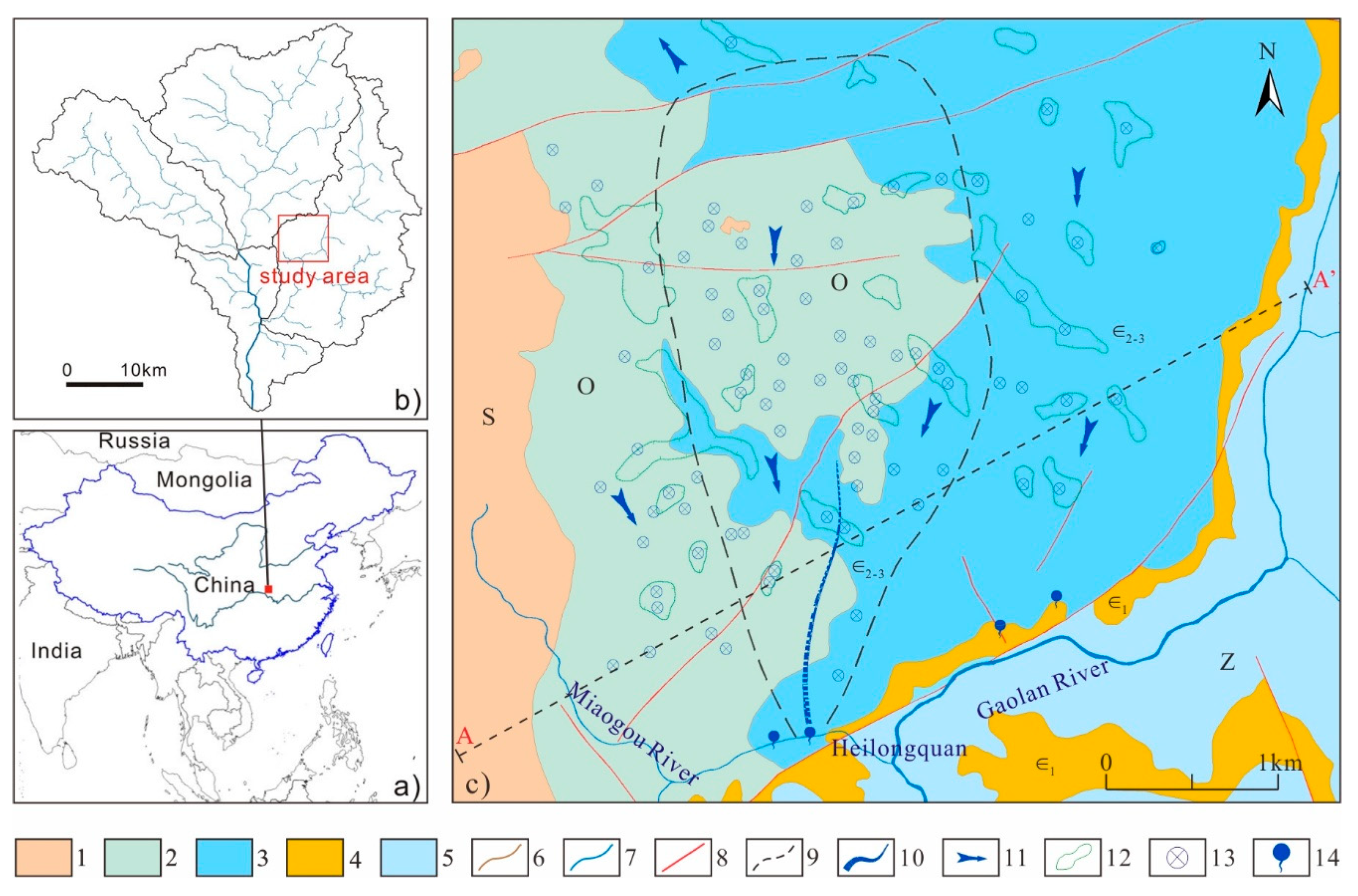
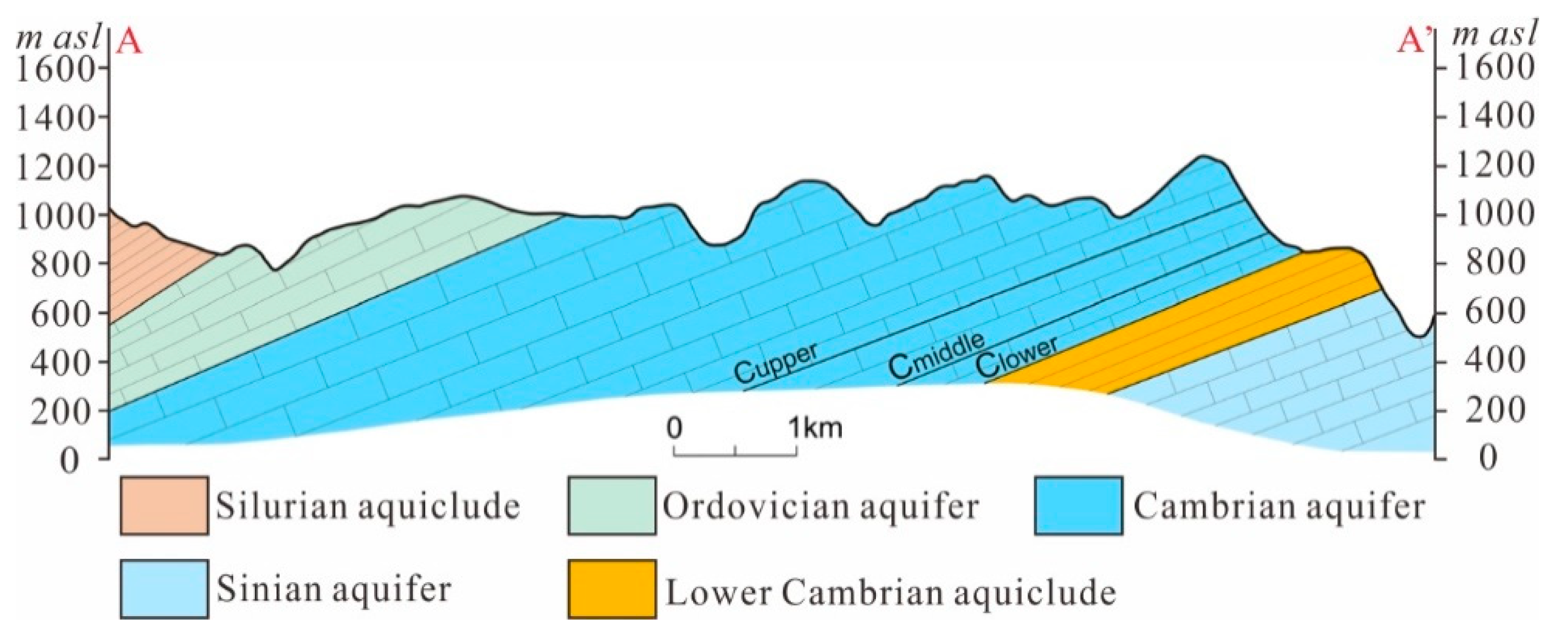
2. Field Site Descriptions
3. Materials and Methods
3.1. Gaussian Mixture Model
3.2. Calculation of Groundwater Runoff Components
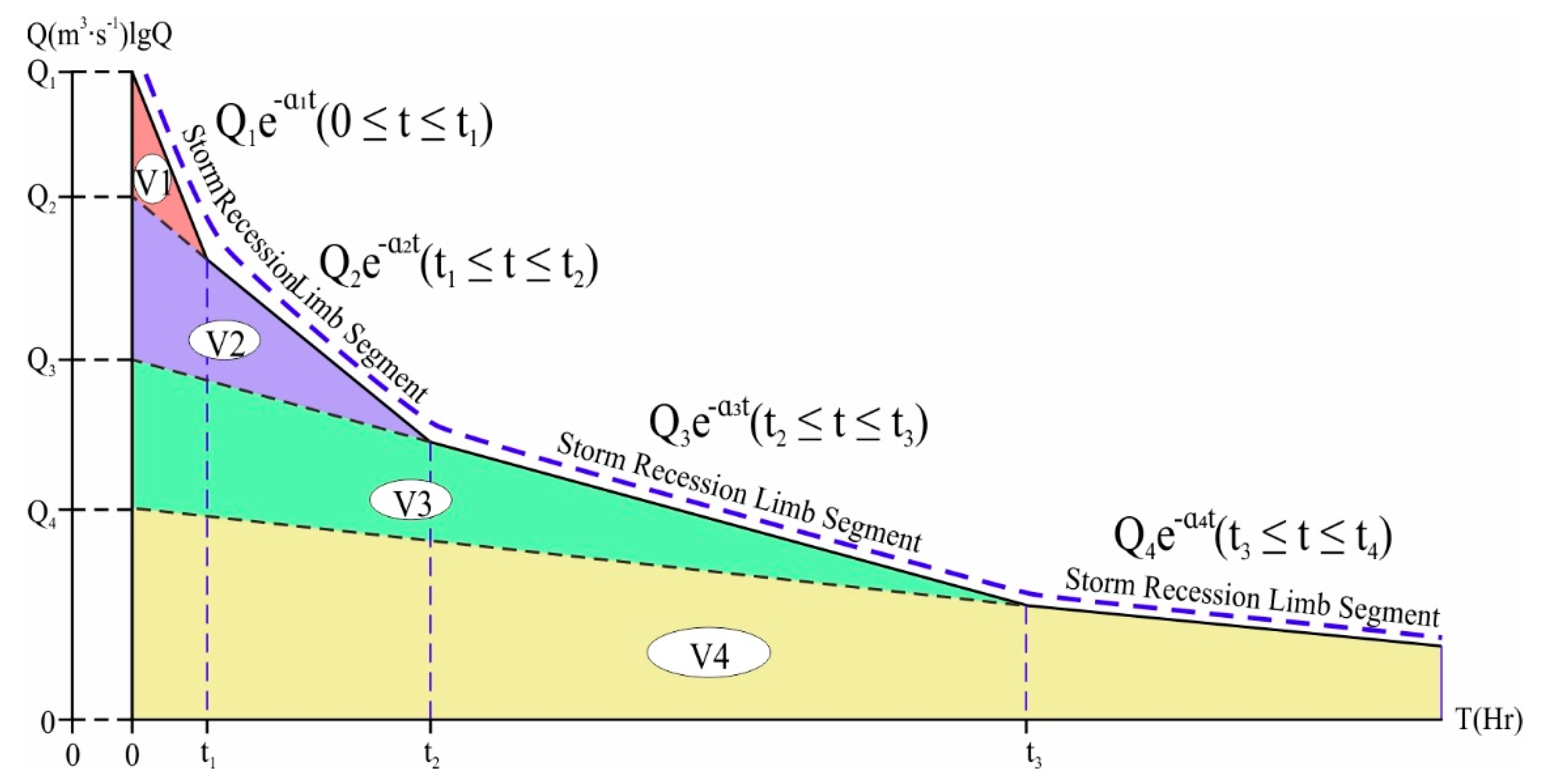
3.3. Hydrograph Recession Analysis
3.4. Data and Materials
4. Results and Discussion
4.1. Conductivity and Discharge of Heilongquan Spring
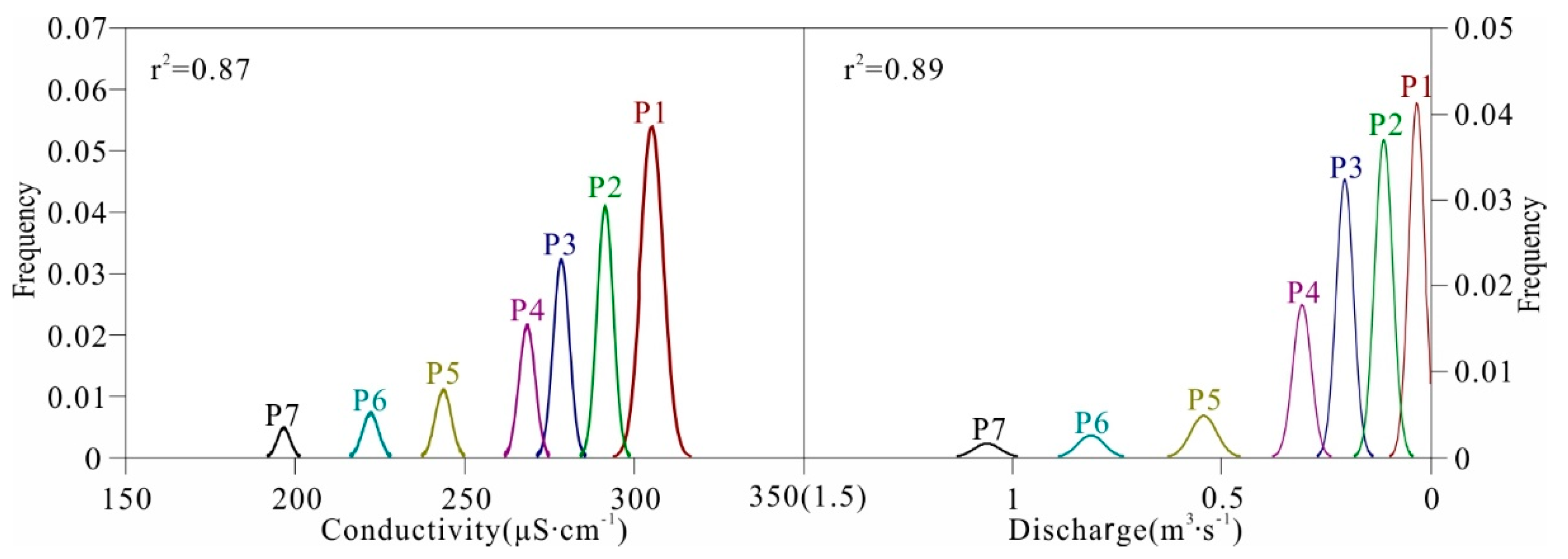
4.2. Identification of Groundwater Runoff Components
4.3. Calculation of Groundwater Runoff Components
4.4. Verification of Calculation Results
5. Conclusions
Author Contributions
Funding
Acknowledgments
Conflicts of Interest
References
- Rusjan, S.; Sapač, K.; Petrič, M.; Lojen, S.; Bezak, N. Identifying the hydrological behavior of a complex karst system using stable isotopes. J. Hydrol. 2019, 577, 123965. [Google Scholar] [CrossRef]
- Zoghbi, C.; Basha, H. Simplified physically based models for free-surface flow in karst systems. J. Hydrol. 2019, 578, 124040. [Google Scholar] [CrossRef]
- Luo, M.; Chen, Z.; Zhou, H.; Jakada, H.; Zhang, L.; Han, Z.; Shi, T. Identifying structure and function of karst aquifer system using multiple field methods in karst trough valley area, South China. Environ. Earth Sci. 2016, 75, 824. [Google Scholar] [CrossRef]
- Boucher, M.; Girard, J.; Legchenko, A.; Baltassat, J.; Dorfliger, N.; Chalikakis, K. Using 2D inversion of magnetic resonance soundings to locate a water-filled karst conduit. J. Hydrol. 2006, 330, 413–421. [Google Scholar] [CrossRef]
- Lauber, U.; Goldscheider, N. Use of artificial and natural tracers to assess groundwater transit-time distribution and flow systems in a high-alpine karst system (Wetterstein Mountains, Germany). Hydrogeol. J. 2014, 22, 1807–1824. [Google Scholar] [CrossRef]
- Gruszczyński, T.; Małecki, J.J.; Romanova, A.; Ziułkiewicz, M. Reconstruction of Thermal Conditions in the Subboreal Inferred from Isotopic Studies of Groundwater and Calcareous Tufa from the Spring Mire Cupola in Wardzyń (Central Poland). Water 2019, 11, 1945. [Google Scholar] [CrossRef]
- Wang, Z.; Zhou, H.; Luo, M.; Guo, X.; Cai, Z. Variations of discharge processes and runoff components between small karst watershed and non-karst watershed in South China. Hydrogeol. Eng. Geol. 2019, 46, 27–39, (with English abstract). [Google Scholar]
- Eris, E.; Wittenberg, H. Estimation of baseflow and water transfer in karst catchments in Mediterranean Turkey by nonlinear recession analysis. J. Hydrol. 2015, 530, 500–507. [Google Scholar] [CrossRef]
- Gil-Márquez, J.; Andreo, B.; Mudarra, M. Combining hydrodynamics, hydrochemistry, and environmental isotopes to understand the hydrogeological functioning of evaporite-karst springs. An example from southern Spain. J. Hydrol. 2019, 576, 299–314. [Google Scholar] [CrossRef]
- Mohammadi, Z.; Illmanb, W.; Karimi, M. Optimization of the hydrodynamic characteristics of a karst conduit with CFPv2 coupled to OSTRICH. J. Hydrol. 2018, 567, 564–578. [Google Scholar] [CrossRef]
- Jeannin, P.; Hessenauer, M.; Malard, A.; Chapuis, V. Impact of global change on karst groundwater mineralization in the Jura Mountains. Sci. Total. Environ. 2016, 541, 1208–1221. [Google Scholar] [CrossRef]
- Massei, N.; Mahler, B.J.; Bakalowicz, M.; Fournier, M.; Dupont, J.P. Quantitative interpretation of specific conductance conductivity frequency distributions in Karst. Groundwater 2007, 45, 288–293. [Google Scholar] [CrossRef]
- Bicalho, C.C.; Guilhe, C.B.; Seidel, J.L.; Exter, S.V.; Jourde, H. Geochemical evidence of water source characterization and hydrodynamic responses in a karst aquifer. J. Hydrol. 2012, 450–451, 206–218. [Google Scholar] [CrossRef]
- Wang, Y.; Guo, Q.; Su, C.; Ma, T. Strontium isotope characterization and major ion geochemistry of karst water flow, Shentou, northern China. J. Hydrol. 2006, 328, 592–603. [Google Scholar] [CrossRef]
- Ptrini, R.; Italiano, F.; Ponton, M.; Slejko, F.; Aviani, U. Geochemistry and isotope geochemistry of the Monfalcone thermal waters (northern Italy): inference on the deep geothermal reservoir. Hydrogeol. J. 2013, 21, 1275–1287. [Google Scholar] [CrossRef]
- Sun, Z.; Ma, R.; Wang, Y.; Ma, T.; Liu, Y. Using isotopic, hydrogeochemical-tracer and temperature data to characterize recharge and flow paths in a complex karst groundwater flow system in northern China. Hydrogeol. J. 2016, 24, 1393–1412. [Google Scholar] [CrossRef]
- Jia, Z.; Zang, H.; Hobbs, P.; Zheng, X.; Xu, Y.; Wang, K. Application of inverse modeling in a study of the hydrogeochemical evolution of karst groundwater in the Jinci Spring region, northern China. Environ. Earth Sci. 2017, 76, 312. [Google Scholar] [CrossRef]
- Wu, X.; Li, C.; Sun, B.; Geng, F.; Gao, S.; Lv, M.; Ma, X.; Li, H.; Xing, L. Groundwater hydrogeochemical formation and evolution in a karst aquifer system affected by anthropogenic impacts. Environ. Geochem. Health 2019, 76, 312. [Google Scholar] [CrossRef]
- Guo, F.; Jiang, G.; Liu, S.; Tang, Q. Identifying source water compositions of karst water systems by quantifying the conductance frequency distribution of springs. A.W.S. 2018, 29, 245–251, (with English abstract). [Google Scholar]
- White, W.B. Conceptual models for karst aquifers. Speleogenesis Evol. Karst Aquifers 2003, 1, 1–6. [Google Scholar]
- Neilson, B.T.; Tennant, H.; Stout, T.L.; Miller, M.P.; Gabor, R.S.; Jameel, Y.; Millington, M.; Gelderloos, A.; Bowen, G.J.; Brooks, P.D. Stream centric methods for determining groundwater contributions in karst mountain watersheds. Water Resour. Res. 2018, 54, 6708–6724. [Google Scholar] [CrossRef]
- Bakalowicz, M. Contribution de la géochimie des eaux à la connaissance de l’ aquifère karstique et de la karstification. Ph.D. Thesis, University of Paris, Paris, France, 1979. [Google Scholar]
- Sa´nchez, D.; Barbera’, J.A.; Mudarra, M.; Andreo, B. Hydrogeochemical tools applied to the study of carbonate aquifers: examples from some karst systems of Southern Spain. Environ. Earth Sci. 2015, 74, 199–215. [Google Scholar] [CrossRef]
- Liu, W.; Brancelj, A. Hydrochemical response of cave drip water to snowmelt water, a case study from Velika Pasica Cave, central Slovenia. Acta Carsologica 2014, 43, 65–74. [Google Scholar] [CrossRef]
- Barbera’, J.A.; Andreo, B. Functioning of a karst aquifer from S Spain under highly variable climate conditions, deduced from hydrochemical records. Environ. Earth Sci. 2012, 65, 2337–2349. [Google Scholar] [CrossRef]
- Minvielle, S.; Lastennet, R.; Denis, A.; Peyraube, N. Characterization of karst systems using SIc-Pco2 method coupled with PCA and frequency distribution analysis. Application to karst systems in the Vaucluse county (Southeastern France). Environ. Earth Sci. 2015, 74, 7593–7604. [Google Scholar] [CrossRef]
- Luo, M.; Chen, Z.; Zhou, H.; Zhang, L.; Han, Z. Hydrological response and thermal effect of karst springs linked to aquifer geometry and recharge processes. Hydrogeol. J. 2018, 26, 629–639. [Google Scholar] [CrossRef]
- Jarvis, B. Statistical Aspects of the Microbiological Examination of Foods, 3rd ed.; Academic Press: Salt Lake City, UT, USA, 2016; pp. 13–45. [Google Scholar]
- Fu, T.; Chen, H.; Wang, K. Structure and water storage capacity of a small karst aquifer based on stream discharge in southwest China. J. Hydrol. 2016, 534, 50–62. [Google Scholar] [CrossRef]
- Bailly-Comte, V.; Martin, J.; Jourde, H.; Screaton, E.; Pistre, S.; Langston, A. Water exchange and pressure transfer between conduits and matrix and their influence on hydrodynamics of two karst aquifers with sinking streams. J. Hydrol. 2010, 386, 55–66. [Google Scholar] [CrossRef]
- Liu, W.; Brancelj, A.; Ellis Burnet, J. Interpretation of cave drip water recession curves, a case study from Velika Pasica Cave, central Slovenia. Hydrol. Sci. J. 2016, 61, 2754–2762. [Google Scholar] [CrossRef]
- Luo, M.; Zhou, H.; Chen, Z. The Law of Karst Water Circulation in Xiangxi River Basin, 1st ed.; Science Press: Beijing, China, 2018; pp. 67–76. [Google Scholar]
- Jakada, H.; Chen, Z.; Luo, M.; Zhou, H.; Wang, Z.; Habib, M. Watershed characterization and hydrograph recession analysis: A comparative look at a karst vs. non-karst watershed and implications for groundwater resources in Gaolan River Basin, Southern China. Water 2019, 11, 743. [Google Scholar] [CrossRef] [Green Version]
- Kresic, N.; Bonacci, O. Spring discharge hydrograph. In Groundwater Hydrology of Springs; Kresic, N., Stevanovic, Z., Eds.; Butterworth-Heinemann: Oxford, UK, 2010. [Google Scholar]


| Water Year | P1 | P2 | P3 | P4 | Pslow | P5 | P6 | P7 | P8 | Pfast | Qm/(m3·s−1) | r2 | δ | |
|---|---|---|---|---|---|---|---|---|---|---|---|---|---|---|
| Gaussian Mixture Model of the Conductivity | ||||||||||||||
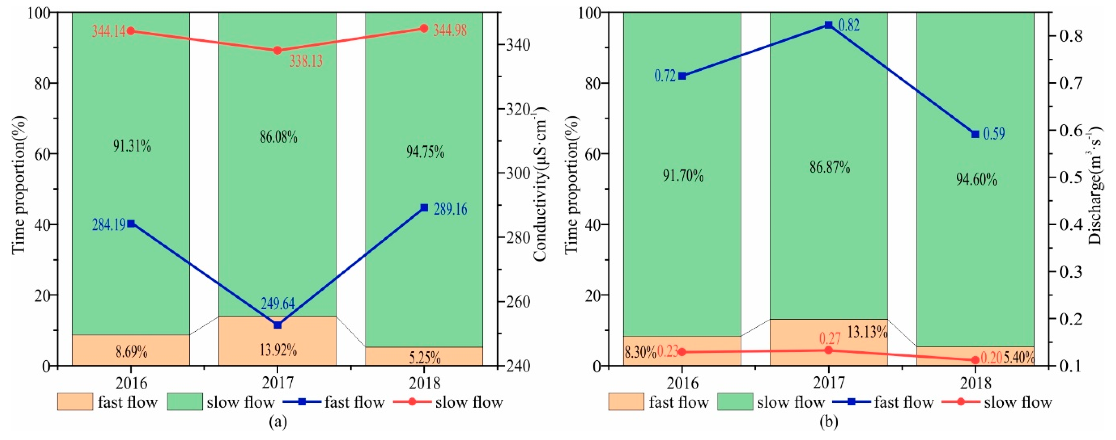
| Time proportion εc/% | 2016 | 53.24 | 18.05 | 12.79 | 7.24 | 91.31 | 5.12 | 3.29 | 0.27 | / | 8.69 | 0.1618 | 0.89 | 0.0038 |
| 2017 | 35.23 | 26.16 | 14.56 | 10.13 | 86.08 | 5.91 | 3.80 | 2.95 | 1.27 | 13.92 | 0.1897 | 0.82 | 0.0045 | |
| 2018 | 34.02 | 26.07 | 19.24 | 15.42 | 94.75 | 3.34 | 1.91 | / | / | 5.25 | 0.1413 | 0.84 | 0.0043 | |
| Mathematical expectation μq/(μS·cm−1) | 2016 | 352.18 | 341.62 | 328.68 | 318.59 | 344.14 | 293.82 | 272.35 | 245.58 | / | 284.19 | 0.1618 | 0.89 | 0.0038 |
| 2017 | 351.18 | 339.59 | 325.55 | 307.04 | 338.13 | 277.54 | 247.03 | 220.38 | 195.57 | 249.64 | 0.1897 | 0.82 | 0.0045 | |
| 2018 | 359.02 | 348.54 | 334.50 | 321.07 | 344.98 | 296.26 | 276.73 | / | / | 289.16 | 0.1413 | 0.84 | 0.0043 | |
| Gaussian Mixture Model of the Discharge | ||||||||||||||
| Time proportion εc/% | 2016 | 30.37 | 24.59 | 20.44 | 16.30 | 91.70 | 4.44 | 2.37 | 1.48 | / | 8.30 | 0.1618 | 0.87 | 0.0019 |
| 2017 | 36.75 | 28.03 | 14.48 | 7.61 | 86.87 | 5.38 | 3.71 | 2.78 | 1.25 | 13.13 | 0.1897 | 0.76 | 0.0049 | |
| 2018 | 30.16 | 25.40 | 21.90 | 17.14 | 94.60 | 3.49 | 1.90 | / | / | 5.40 | 0.1413 | 0.79 | 0.0024 | |
| Mathematical expectation μq/(m3·s−1) | 2016 | 0.07 | 0.13 | 0.20 | 0.25 | 0.13 | 0.55 | 0.82 | 1.06 | / | 0.72 | 0.1618 | 0.87 | 0.0019 |
| 2017 | 0.07 | 0.14 | 0.20 | 0.27 | 0.13 | 0.57 | 0.83 | 1.10 | 1.27 | 0.82 | 0.1897 | 0.76 | 0.0049 | |
| 2018 | 0.04 | 0.10 | 0.15 | 0.20 | 0.11 | 0.50 | 0.76 | / | / | 0.59 | 0.1413 | 0.79 | 0.0024 | |
| Water Year | 2016 | 2017 | 2018 | |||||||||
|---|---|---|---|---|---|---|---|---|---|---|---|---|
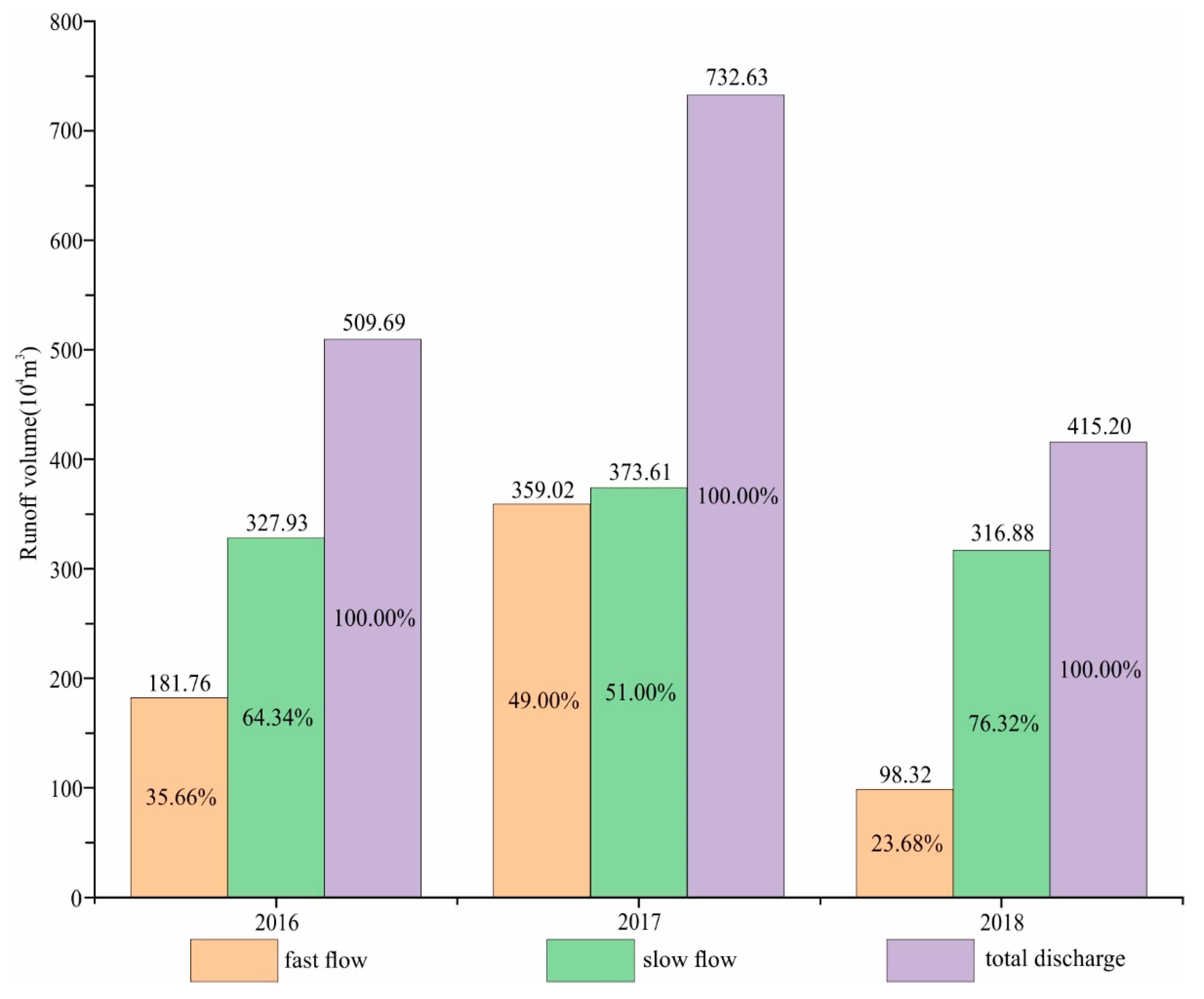
| Slow flow | Time proportion/% | Average discharge/(m3·s−1) | Runoff volume/(104 m3) | Runoff proportion/% | Time proportion/% | Average discharge/(m3·s−1) | Runoff volume/(104 m3) | Runoff proportion/% | Time proportion/% | Average discharge/(m3·s−1) | Runoff volume/(104 m3) | Runoff proportion/% |
| P1 | 53.24 | 0.07 | 114.20 | 22.41 | 35.23 | 0.07 | 82.55 | 11.27 | 34.02 | 0.04 | 47.19 | 11.37 |
| P2 | 18.05 | 0.13 | 74.37 | 14.59 | 26.16 | 0.14 | 112.39 | 15.34 | 26.07 | 0.10 | 78.95 | 19.01 |
| P3 | 12.79 | 0.20 | 81.67 | 16.02 | 14.56 | 0.20 | 92.70 | 12.65 | 19.24 | 0.15 | 91.81 | 22.11 |
| P4 | 7.24 | 0.25 | 57.69 | 11.32 | 10.13 | 0.27 | 85.98 | 11.74 | 15.42 | 0.20 | 98.93 | 23.83 |
| Total up | 91.31 | 0.10 | 327.93 | 64.34 | 86.08 | 0.12 | 373.61 | 51.00 | 94.75 | 0.10 | 316.88 | 76.32 |
| Fast flow | Time proportion/% | Average discharge/(m3·s−1) | Runoff volume/(104 m3) | Runoff proportion/% | Time proportion/% | Average discharge/(m3·s−1) | Runoff volume/(104 m3) | Runoff proportion/% | Time proportion/% | Average discharge/(m3·s−1) | Runoff volume/(104 m3) | Runoff proportion/% |
| P5 | 5.12 | 0.55 | 88.09 | 17.28 | 5.91 | 0.57 | 106.58 | 14.55 | 3.34 | 0.50 | 52.60 | 12.67 |
| P6 | 3.29 | 0.82 | 84.69 | 16.62 | 3.80 | 0.83 | 99.22 | 13.54 | 1.91 | 0.76 | 45.72 | 11.01 |
| P7 | 0.27 | 1.06 | 8.97 | 1.76 | 2.95 | 1.10 | 102.55 | 14.00 | / | / | / | / |
| P8 | / | / | / | / | 1.27 | 1.27 | 50.67 | 6.92 | / | / | / | / |
| Total up | 8.69 | 0.06 | 181.76 | 35.66 | 13.92 | 0.11 | 359.02 | 49.00 | 5.25 | 0.03 | 98.32 | 23.68 |
| Total of all | 100.00 | 0.16 | 509.69 | 100.00 | 100.00 | 0.23 | 732.63 | 100.00 | 100.00 | 0.13 | 415.20 | 100.00 |
| Water Year | 2016 | 2017 | 2018 | ||||||
|---|---|---|---|---|---|---|---|---|---|
| Runoff Volume/(104 m3) | QF | QS | QT | QF | QS | QT | QF | QS | QT |
| Frequency distribution | 181.76 | 327.93 | 509.69 | 359.02 | 373.61 | 732.63 | 98.32 | 316.88 | 415.20 |
| Recession analysis | 169.70 | 311.41 | 481.11 | 328.25 | 350.60 | 678.85 | 85.13 | 302.57 | 387.70 |
| Relative error/% | 6.63 | 5.04 | 5.61 | 8.57 | 6.16 | 7.34 | 13.42 | 4.52 | 6.62 |
© 2019 by the authors. Licensee MDPI, Basel, Switzerland. This article is an open access article distributed under the terms and conditions of the Creative Commons Attribution (CC BY) license (http://creativecommons.org/licenses/by/4.0/).
Share and Cite
Wang, Z.; Chen, Q.; Yan, Z.; Luo, M.; Zhou, H.; Liu, W. Method for Identifying and Estimating Karst Groundwater Runoff Components Based on the Frequency Distributions of Conductivity and Discharge. Water 2019, 11, 2494. https://doi.org/10.3390/w11122494
Wang Z, Chen Q, Yan Z, Luo M, Zhou H, Liu W. Method for Identifying and Estimating Karst Groundwater Runoff Components Based on the Frequency Distributions of Conductivity and Discharge. Water. 2019; 11(12):2494. https://doi.org/10.3390/w11122494
Chicago/Turabian StyleWang, Zejun, Qianlong Chen, Ziqi Yan, Mingming Luo, Hong Zhou, and Wei Liu. 2019. "Method for Identifying and Estimating Karst Groundwater Runoff Components Based on the Frequency Distributions of Conductivity and Discharge" Water 11, no. 12: 2494. https://doi.org/10.3390/w11122494