Particle-Based Workflow for Modeling Uncertainty of Reactive Transport in 3D Discrete Fracture Networks


1
Graduate Institute of Applied Geology, National Central University, Taoyuan City 32001, Taiwan
2
Center for Environmental Studies, National Central University, Taoyuan City 32001, Taiwan
*
Author to whom correspondence should be addressed.
Water 2019, 11(12), 2502; https://doi.org/10.3390/w11122502
Submission received: 28 October 2019
/
Revised: 22 November 2019
/
Accepted: 23 November 2019
/
Published: 27 November 2019
(This article belongs to the Section Hydrology)
Abstract
:Fractures are major flow paths for solute transport in fractured rocks. Conducting numerical simulations of reactive transport in fractured rocks is a challenging task because of complex fracture connections and the associated nonuniform flows and chemical reactions. The study presents a computational workflow that can approximately simulate flow and reactive transport in complex fractured media. The workflow involves a series of computational processes. Specifically, the workflow employs a simple particle tracking (PT) algorithm to track flow paths in complex 3D discrete fracture networks (DFNs). The PHREEQC chemical reaction model is then used to simulate the reactive transport along particle traces. The study illustrates the developed workflow with three numerical examples, including a case with a simple fracture connection and two cases with a complex fracture network system. Results show that the integration processes in the workflow successfully model the tetrachloroethylene (PCE) and trichloroethylene (TCE) degradation and transport along particle traces in complex DFNs. The statistics of concentration along particle traces enables the estimations of uncertainty induced by the fracture structures in DFNs. The types of source contaminants can lead to slight variations of particle traces and influence the long term reactive transport. The concentration uncertainty can propagate from parent to daughter compounds and accumulate along with the transport processes.
1. Introduction
Fractures are important flow paths for solute transport in fractured rocks. Characterizing fracture networks requires knowledge of fracture properties, including fracture numbers, sizes, orientation, and most importantly, the fracture intensity and apertures [1,2,3]. Typical approaches to obtain the fracture properties rely on building statistical structures of the fractures that are similar to those of scanline or window samplings on sites. The statistical structures of the fractures enable the generations of discrete fracture networks (DFNs) for flow and transport simulations. Considering all of the various fracture properties in rock formations is logical but is technologically difficult for practical applications [4]. Investigations have reported that the challenges came with the technical issues in meshing DFNs and in solving flow and transport equations for DFNs [5,6,7]. Moreover, the flow and concentration uncertainty problems due to variation is a common issue and has been considered to quantify the impact on heterogeneous aquifer systems [8,9,10].
Long et al. (1985) were the first to propose the 3D DFN consisting of disk-shaped or polygonal fractures [11]. In recent years, intensive research has developed numerous DFN models to simulate the flow or transport in DFNs [1,4,12,13,14,15]. In these models, the particle tracking (PT) algorithms are usually preferred to simulate DFN flow paths and transport and enable the implementations of evaluating resistance time of contaminants in fractured rocks [12,16,17,18,19]. The advantage of the PT is to avoid numerical difficulties in solving the advection dispersion equation (ADE) for complex DFN domains. In the PT approaches, the released particles in DFNs are assumed to carry contaminants and travel with the flow in fractures. The contaminant in a particle can be treated as specified mass or concentration. The calculation of concentration in a control volume then relies on the collected total mass or concentration from particles in the control volume. Many previous studies have discussed the issues in treating particle movements in fracture rocks with different scales and practical complexity [12,16,18,19,20,21]. These PT approaches mainly focused on the statistics of particle travel times and quantified the influence of fracture properties on the particle movements in DFNs. Advanced features such as the reactive transport in fractured rocks have been under development in recent years [22,23,24].
In fractured porous media, contaminant transport is important in the disposal of chemical and nuclear wastes such as radionuclide wastes, nitrate products, and chlorinated compounds. The contaminants of tetrachloroethylene (PCE) is commonly used for dry cleaning of fabrics, while trichloroethylene (TCE) is commonly used as an industrial solvent for various products [25,26,27]. Over the past decades, the groundwater contaminated by PCE or TCE has become an important environmental issue. These contaminants are typically presented as dense non-aqueous phase liquids (DNAPLs) when sufficient quantities are spilled in groundwater systems [25,28]. The contaminants could migrate into shallow fractured rock systems and make the chemical treatments or bioremediations difficult because of the high heterogeneity of the fractured media [29,30]. How and what degree the influence of the chemical reactions on the contaminant transport are interesting issues for environmental engineers to quantify the plume migrations.
Motivated by the requirement to conduct reactive transport in DFNs, the objective of the study is to develop and test a numerical workflow that enables the simulations of flow, reactive transport, and concentration uncertainty in complex 3D DFNs. Taking advantage of current developments on the PT approaches in fractured media, the study employs the commercialized software FracMan to conduct 3D DFN generations and simulate flow and PT for the generated DFNs [16,31,32,33,34,35,36]. The particle traces obtained from the PT method are extracted and converted to the input files for modeling reactive transport. Specifically, the study considers each particle trace a 1D domain and simulates reactive transport by using the well-developed PHREEQC model. The 1D particle traces are discretized to fit the computational requirements in PHREEQC [37]. Results of the reactive transport along particle traces are then mapped in the 3D DFNs to present the migration processes of the contaminations, including the concentration of parent and daughter compounds. Converting the input and output files for the PHREEQC model and mapping the results in the 3D DFNs are efficiently executed by using the developed VBA script in this study.
2. Materials and Methods
The workflow takes advantage of recent developments in the fields of DFN generations, DFN flow simulations, and reactive transport modeling. The following sections briefly detail the concept of the proposed workflow and the associated technical issues involved in the workflow. The details of fracture properties for DFN generations and flow simulations and the particle tracking algorithm are also described. In this study, the effort has been devoted to developing a program to convert input and output files and execute the PHREEQC model. The FracMan/MAFIC and PHREEQC are main models used in the study. FracMan/MAFIC was developed by Golder Associates Inc. in order to perform discrete features, flow, and solute transport in 3D fracture porous media [38]. The package has been verified and validated with various cases and employed to several relevant studies [6,38]. Additionally, PHREEQC is a computer program written in the C programming language that is designed to perform a wide variety of aqueous geochemical calculations. The program was released and maintained by USGS. The model had been verified and validated by the model developers and users [37].
2.1. Workflow
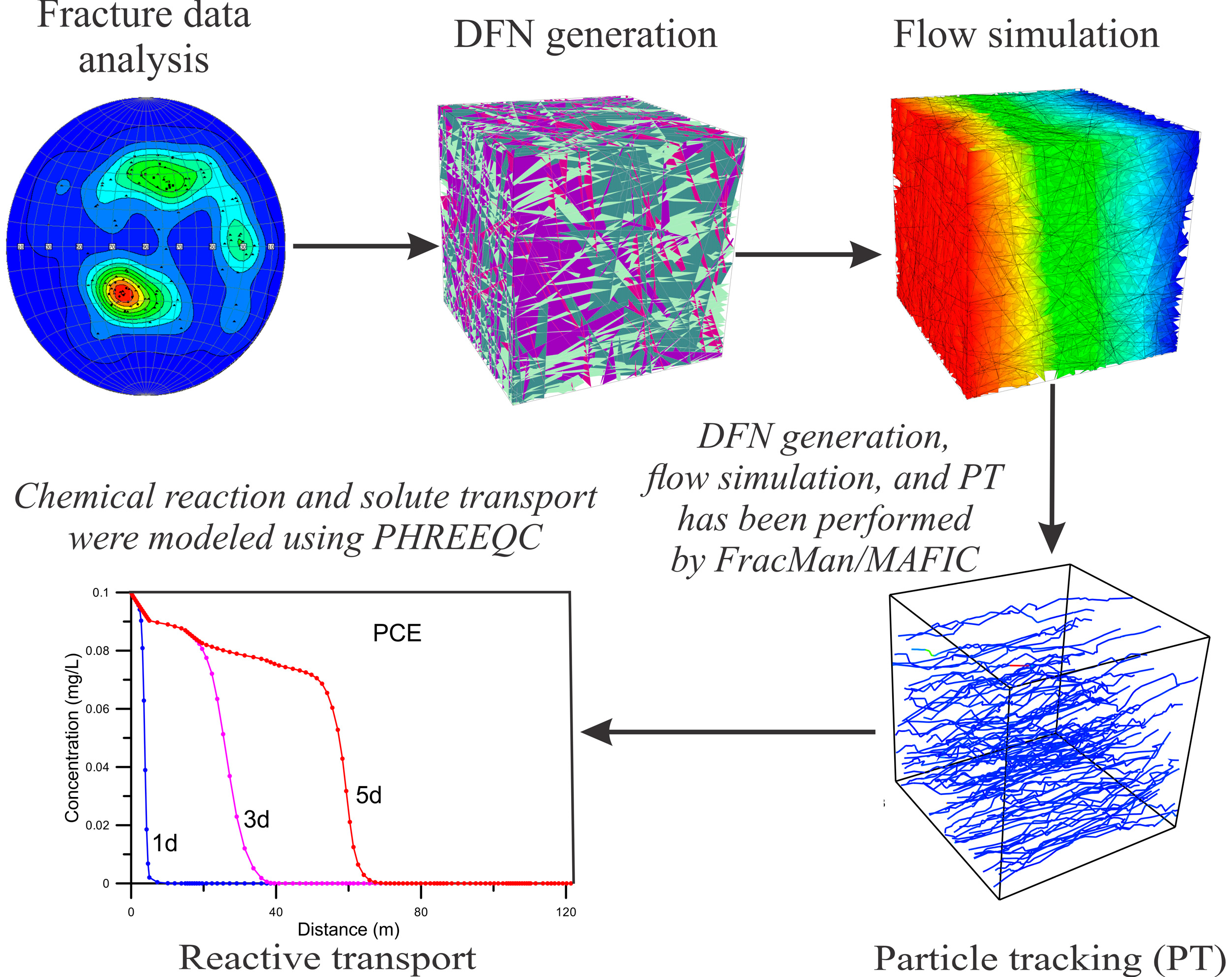
The workflow consists of four main steps, including the DFN generation, DFN flow simulation, DFN particle tracking, and reactive transport along particle traces. Figure 1 presents the concept and the main steps involved in the workflow. In the workflow, FracMan software is used to build 3D DFN based on the fracture properties obtained from site-specific samplings. The generated DFN provides detailed information about fracture geometries, sizes, locations, and connections. A mesh generation process is then conducted to discretize the generated DFN. Simulation of DFN flow is based on the numerical finite element model MAFIC modified by Miller et al. (2001) [38]. The MAFIC is a well-known code for flow and transport simulation and widely used for several researches [38]. Conducting PT tracking relies on the mesh and fracture locations and the flow field in the 3D DFN. The FracMan software allows the particles to be randomly released on a specified plane, along with a line, or in a defined volume. The PT tool in FracMan provides detailed particle traces in the domain of the 3D DFN and the particle traces are extracted and discretized to provide numerical parameters for the PHREEQC model. The challenging task in executing the PHREEQC model for particle traces is the discretization of particle traces because the particle paths and movement steps can vary differently from one to another. In this study, we used all the particles released in the 3D DFN. However, due to computational efficiency we excluded the particles that move into dead ends. This process yields the same number of PHREEQC simulations as the number of selected particle traces in the simulation domain of the 3D DFN.
2.2. DFN Flow and Particle Tracking
The generation of DFNs requires the information of individual fractures, including the orientation, size, shape, and aperture. Each fracture property can follow a given probability distribution as well as the topological relationship between fractures and fracture sets [39]. Many previous studies have focused on the statistical description of fracture properties, including fracture distributions [40], lengths, apertures [41], orientations, and other parameters [42]. In this study, the selected fracture properties for the DFN generation are the Fisher probability model for fracture orientations [43,44]:
where is the distribution parameter (Fisher constant or the dispersion factor) and is the deviation angle from the mean pole. The fractures generator uses the fracture sets obtained from the site-specific samplings.
In this study, the generated fracture is defined by two facing rock surfaces. We assume that the two surfaces are two rough parallel plates that enable fluid to pass through the plates with relatively high velocity [1,45]. Pruess and Tsang (1990) proposed a similar concept for their numerical model [46]. In their study, the fractures were assumed to have rough surfaces with numerous contact points and the fractures consist of the void space enclosed between two impermeable surfaces, which constitutes a two-dimensional porous medium in a topological sense. The concept of the porous medium in a fracture plate was then employed in this study for 3D DFNs. Note that this study only focused on the flow and transport in fractures and neglected the interactions of fractures and the surrounding rock matrix. The FracMan software has integrated the MAFIC model to simulate flow through the porous fractures. The flow equation in fractured rocks employs the mass conservation concept and Darcy’s law [6,38,47]:
where is specific storage [1/L] and is the hydraulic head [L]. The notation is the hydraulic conductivity [L/T] and the notation is the source or sink term applied to aquifers [1/T]. In Equation (2), t is time [T] and is the Laplace operator. In this work, the specified head and no flow boundary conditions were used for the simulations.
The particle tracking (PT) approach is a well-developed technique used for efficient determination of advective transport in complex DFNs [34]. Previous investigations have shown the advantages of the PT approach for complex DFN flow systems. The PT approach relies on the flow field obtained from Equation (2) [48]. In the DFN, the particles are randomly released in the simulation domain. The flow field provides seepage velocity at each node of the finite element mesh in the DFN. The particle movements are then determined based on the linear interpolation of velocities at surrounding finite element nodes near a particle. For a specified time step, the particle movements can be different because of the velocity variations in the DFN flow field. Note that the particle movements are restricted in the fracture plates in a DFN. In this study, the simulations of reactive transport require the information recorded along the particle traces.
2.3. Advection–Reaction–Dispersion Model
PHREEQC is a well-developed computer program to perform various simulations of geochemical reactions [37]. This study employed the PHREEQC to model 1D reactive transport based on the particle traces obtained from the DFN flow fields. The governing equation for transport in the DFN flow system can be described by the following 1D advection reaction dispersion (ARD) equation [37]:
where [M/L3] is the concentration and [L/T] is the seepage velocity. The notation [L2/T] represents the dispersion coefficient. The term in Equation (3) refers to the advection process and the term refers to the dispersion process. The represents the change of concentration influenced by the reactions. We assume that the seepage velocity is the same for all of the solute species. Similarly, the dispersion coefficient is a fixed value for all species.
For the chemical reaction process, this study considers chemical kinetics to be the transport process. The concentration change with time follows the rate equation:
where is the stoichiometric coefficient of species in the kinetic reaction. Notation represents the overall reaction or substance (mol/kgw/s). The PHREEQC model calculates the rate with time by using Runge–Kutta numerical method. The overall rate of kinetic reaction is defined by the equation:
where is the specific rate (mol/m2/s), is the initial surface area (m2), and is the volume of solution (kgw). The notations and are the initial moles and the moles at a given time, respectively. In Equation (5), the term is a factor to account for the change of .
2.4. Integration of PT and the PHREEQC Model
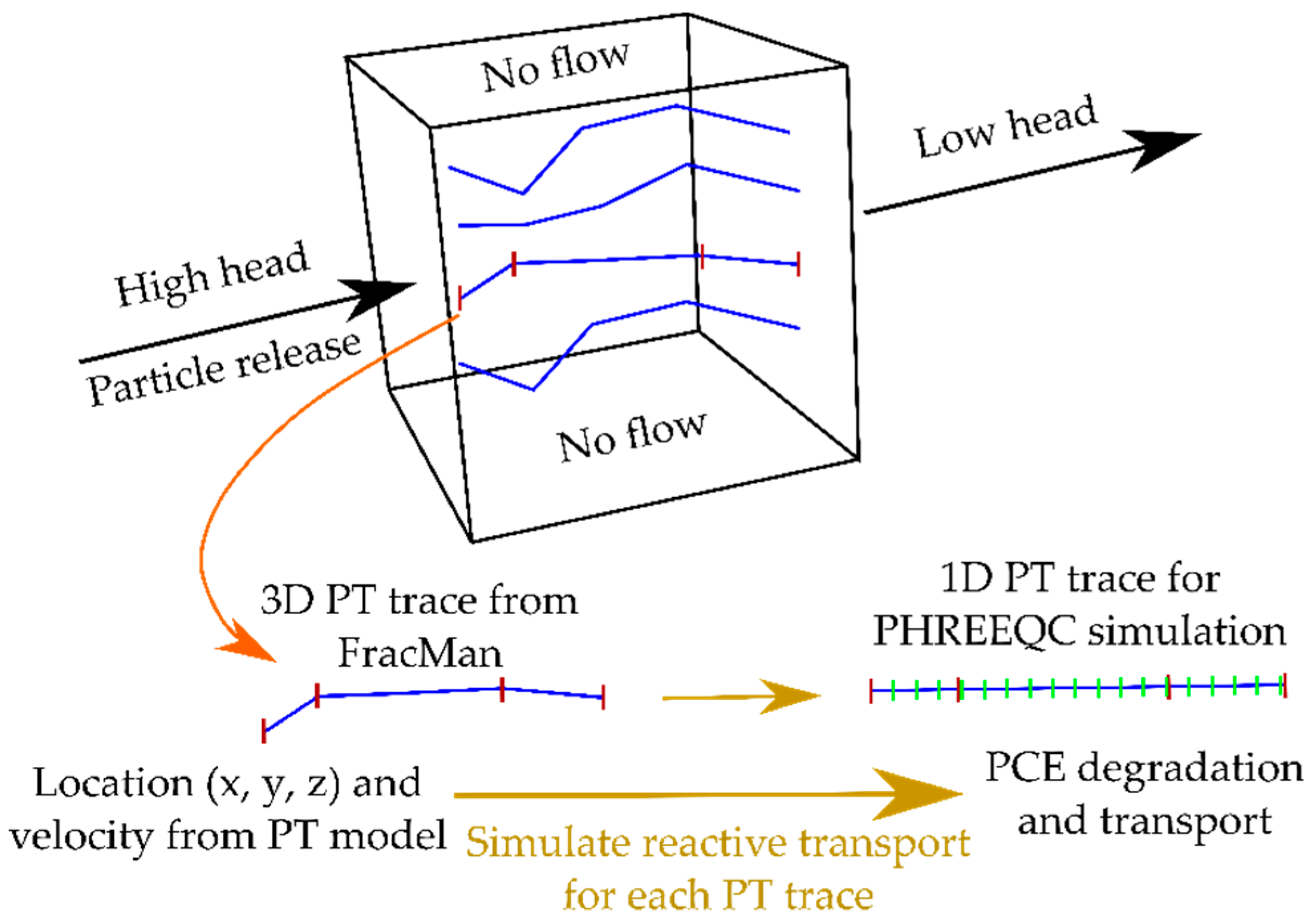
Figure 2 shows the detailed procedures for integrating PT and PHREEQC simulations. In the PT simulations, the particles are released in the upstream area either located at specified points or randomly placed in the fractures. Extracted particle traces from the PT approach aim to obtain 1D flow pathways for modeling reactive transport in PHREEQC. Note that the particle traces involve numerous segments, which indicate the particle movements of different time steps in the DFN. The segments in the particle traces might be nonuniform, depending on the local velocity field in the DFN. This study developed a VBA script to read and reformulate the input files for the PHREEQC model. To prepare the required information for PHREEQC simulations, the particle traces from PT approaches are divided into several uniform cells in different segments of the particle traces (see Figure 2). We assume that the seepage velocity in each segment of particle traces is constant. All other transport and reaction parameters are assigned to each cell in the segments. The PHREEQC model includes all the segments in a particle trace to complete the simulation of 1D reactive transport. To present the results from the PHREEQC simulations for DFNs, the study shows the concentration distribution along the particle traces. However, the coordinates of the particle traces follow the pathways in the 3D DFN. With many PTs conducted in the 3D DFN, the variations of concentration can be obtained for complex fractured flow systems.
3. Numerical Examples
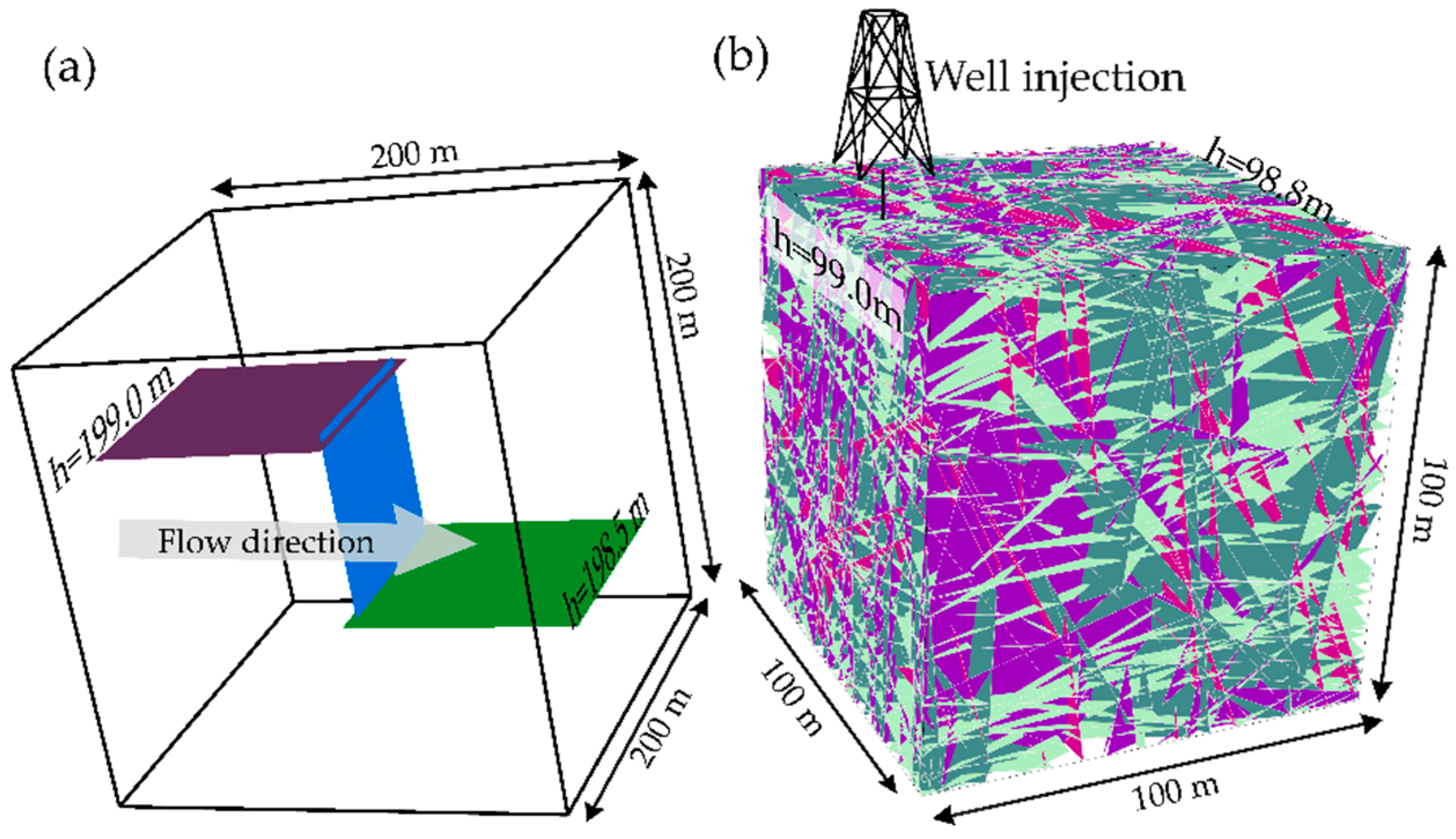
The objective of the study is to develop an efficient workflow that can conduct flow and reactive transport in complex fracture networks. Specifically, we take the advantages of the recent development in 3D DFN generation, fracture flow simulation, and particle tracking. The workflow integrates the solutions from MAFIC and PHREEQC models and makes simulations of reactive transport feasible in DFNs. This study used three numerical examples to illustrate the developed workflow. The first case (i.e., Case 1) consists of a simple connection of fractures in a simulation domain (see Figure 3a). In this case, we aim to test and assess the results obtained from the workflow.
The second and third cases (i.e., Cases 2 and 3) involved complex fracture sets sampled from a site in Taiwan. There is a fractured granite located near the land surface of the site (see Figure 3b). The depth to the granite is small so that the source of surface contamination might threaten the groundwater environment near the site. This study focuses on the flow and transport in the saturated zone of the near-surface granite. It is interesting to understand the plume migration and reactive transport in the fractured formation. Additionally, we aim to assess the propagation of concentration uncertainty induced by the specified fracture structure obtained at the site. The uncertainty represents the variations of contaminants that flow out of the porous fractures. In Cases 2 and 3, we consider the fixed domain size, boundary conditions, and the fracture sets, while the release of particles (i.e., source plumes) are different. In Case 2 the source of contaminant will be randomly distributed on the face of the upstream boundary. Case 3 involves a well that creates a line source of concentration for transport simulation. Figure 3b shows the location of the well (x = 10, y = 50) that provides a line source concentration along the well. The well is opened from the depth of 30 m to the depth of 70 m for injecting contaminant. In the simulation cases, the source contaminant is assumed to be the PCE degradation applied to the 1D PHREEQC simulations.
3.1. Model Parameters and Numerical Considerations
The modeling size for Case 1 is a 200 × 200 × 200 m domain, while the domain size for Case 2 and Case 3 is 100 × 100 × 100 m (see Figure 3). Constant heads are specified on upstream and downstream boundary faces to create background head gradients for flow from the west to the east boundaries. The no-flow boundary condition was applied to other boundaries. In this study, we consider a fixed fracture transmissivity in each case. Table 1 lists the fracture parameters for DFN flow simulations in three different cases. There are four sets of fractures used to generate the complex DFN for Case 2 and Case 3. The study conducts the steady state flow simulations for all cases. In Case 1, we release 50 particles along the edge of the horizontal fracture on the upstream boundary. However, there are 100 particles used for the simulations of reactive transport in the complex DFN cases (i.e., in Cases 2 and 3). Similar to the particle locations in Case 1, in Case 2 the particle locations are randomly located on the fracture edges that intersect with the upstream boundary faces. Additional flow direction (i.e., the y-direction from the south to the north boundary faces) was tested in Case 2 to assess the influence of the fracture structure on the behavior of particle travel times. In Case 3, the locations of the released particles are determined based on the intersection points between fractures and the defined vertical line at the well location (x = 10, y = 50).
3.2. Parameters for PHREEQC Reactive Transport
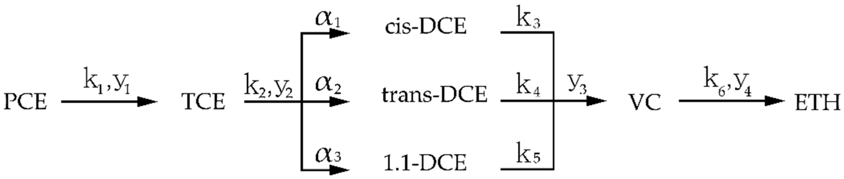
In this study, the workflow includes the PHREEQC simulation applied to each particle trace obtained from the MAFIC model. We consider the well-known PCE degradation for all cases in this study. The PCE is one of common VOCs that undergoes a degradation process since reducing conditions, mainly by microbiological transformations. The most important pathways for biodegradation of PCE is by sequential reductive dechlorination [49]. There are six components in this pathway, including PCE, TCE, cis-1,2-dichloroethylene (cis-DCE), trans-1,2-dichloroethylene (trans-DCE), 1,1-dichloroethylene (1,1-DCE), and vinyl chloride (VC). Figure 4 shows the degradation pathway of PCE based on the first-order rate constants. The particle traces and the associated seepage velocity along the particle traces provide input data for PHREEQC models. Table 2 lists the computational parameters for PHREEQC transport simulations. Table 3 shows the parameters for PCE biodegradation. In this study, we model the migration of PCE contaminant based on the condition of the continuous injection source.
4. Results and Discussion
4.1. Test of the Workflow
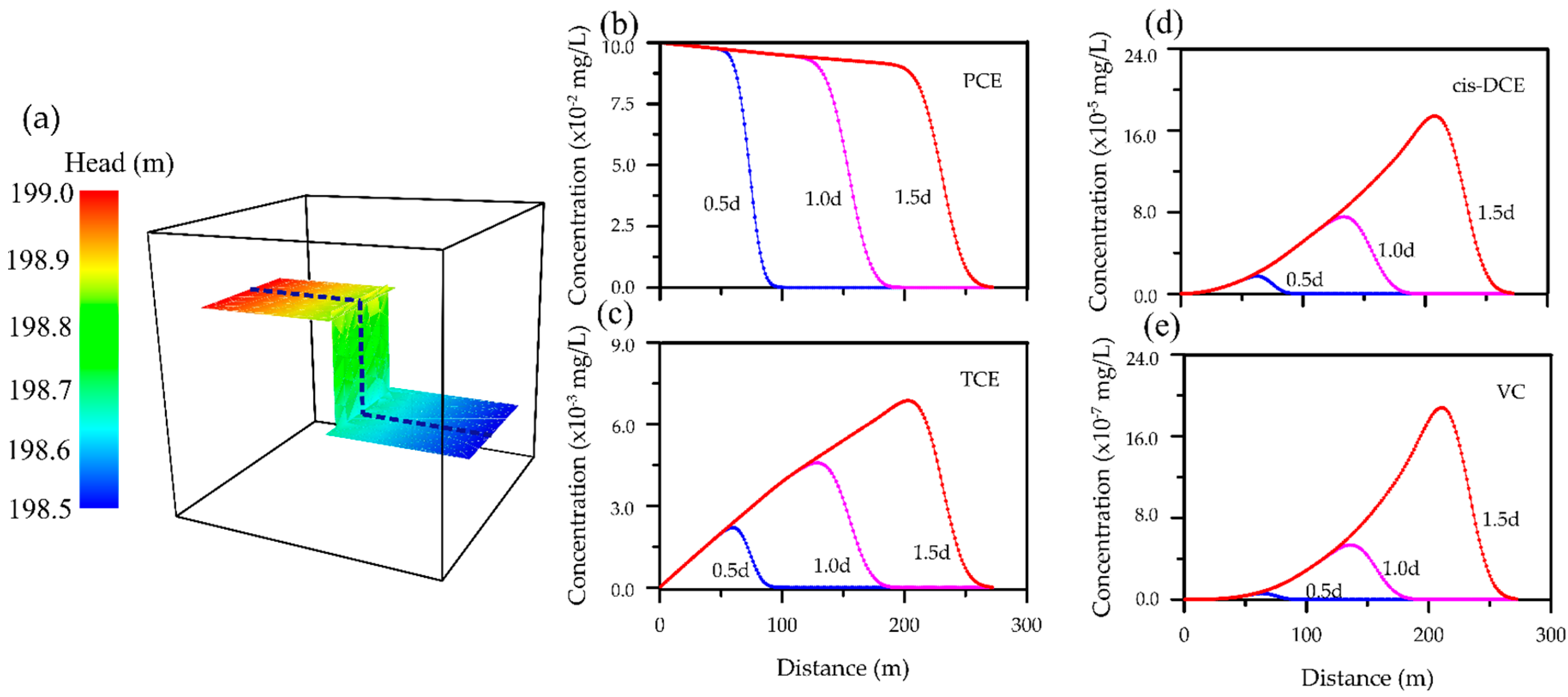
We used Case 1 to illustrate the developed workflow for modeling flow and reactive transport in 3D DFNs. There were three fractures connected in the simulation domain. However, the width of the three fractures were different. Figure 5a shows the head distribution for the steady state flow. Based on the constant heads assigned to the east and the west boundaries, a background head gradient of 0.0025 yielded the head that gradually changed from the west to the east boundary. Using the PT results, the continuous PCE source was specified with a constant concentration of 0.1 mg/L at the inlet boundary. Figure 5b,c shows the concentration of PCE degradation along a selected particle trace (see dashed line in Figure 5a). Figure 5b presents the distributions of PCE concentration at different times. The Case 1 considered the continuous injection of PCE at the west boundary. The results in Figure 5b show that the PCE concentration along the particle trace decreases with the distance. However, the concentration of other compounds gradually increases with time and distance. In this case, the particle traces were longer than the horizontal domain size because a vertical fracture was placed perpendicular to the two horizontal fractures (see Figure 5a).
We collected the concentration for the 50 particles and plotted the distribution of the concentration along the particle traces. Figure 6 shows the results for concentration at t = 1.0 day. The results clearly show that the concentration distribution for all particles is nearly identical (the light color lines). The mean values and the particle paths exhibit small variations. For a specified time, we estimated the uncertainty (i.e., the standard deviation, STD) at each location along the particle trace. The small variations might be induced by inconsistencies of the fracture connection. In the case, the widths of the three fractures are not the same so that the flow field shows slight variability near the two ends of fracture intersection lines. The varied flow field, therefore, triggers the variations of concentration in the fractures. In Figure 6a, we obtain a small variation of PCE concentration uncertainty near the concentration front, where the concentration changes significantly along the particle traces (see standard deviation line in Figure 6a). We define the zone as the main uncertainty peak (MUP) in this study. The result is similar to the general understanding of contaminant transport in porous media. However, in this study, an area with an additional high uncertainty value was obtained for the production compounds (see standard deviation line in Figure 6b–d). We further define this small uncertainty variation as the secondary uncertainty peak (SUP). By comparing the results for t = 1.0 day in Figure 5c–e, these areas also indicate the zones with the high variation of concentration for production compounds. The results from the test example demonstrate that the uncertainty can propagate from the parent to the daughter compounds.
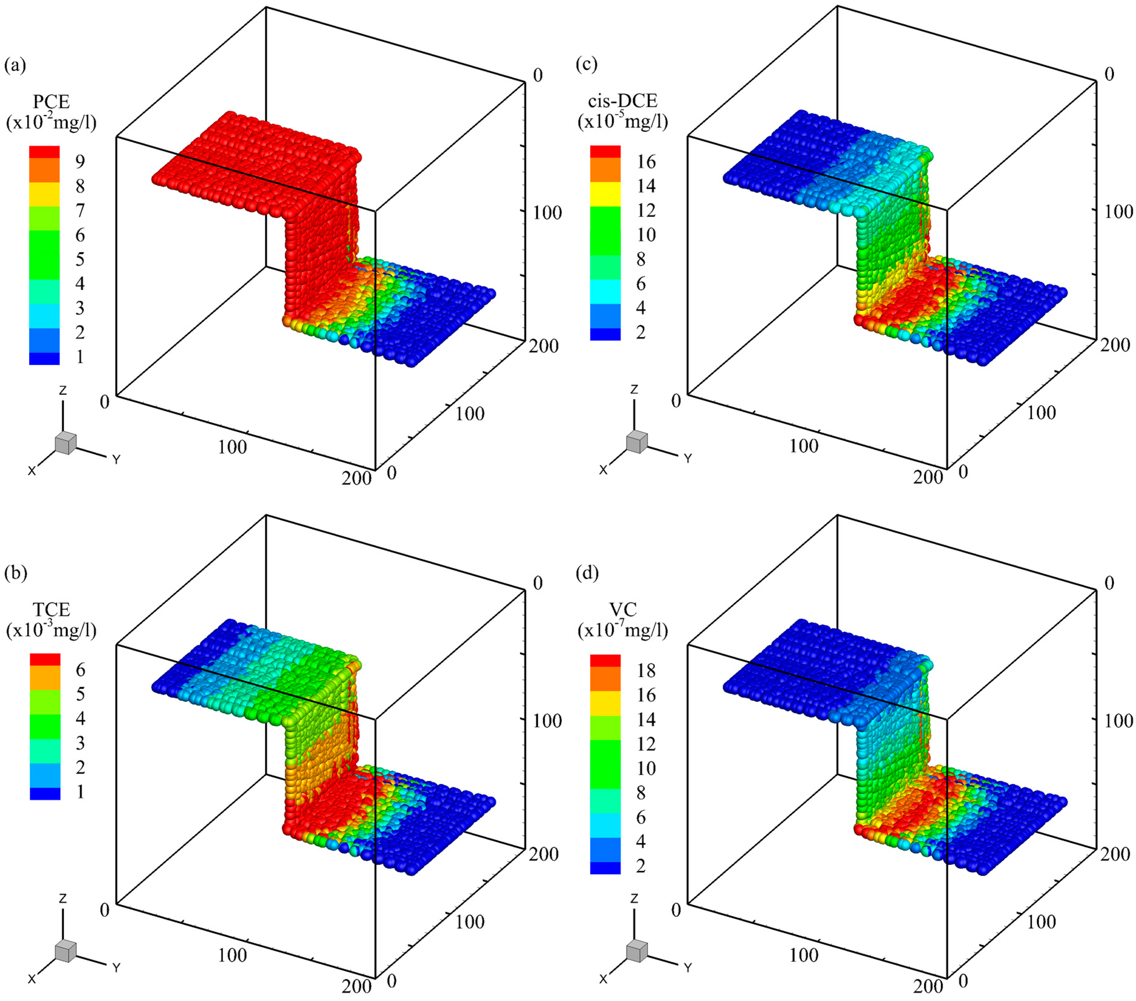
The results for 50 particles were then recorded and plotted in the 3D DFN domain. Figure 7 shows the 3D distributions of different concentration at t = 1.5 day. The promising results enabled us to assess reactive transport in a 3D DFN flow system. Case 1 provided a simple fracture connection. In this case, we released 50 particles for demonstration purposes. For cases with practical complexity, more particles might be required to obtain a better representation of transport behavior in fractured rocks. The following cases will present the scenarios.
4.2. DFN Flow and Travel Time Statistics for the Released Particles
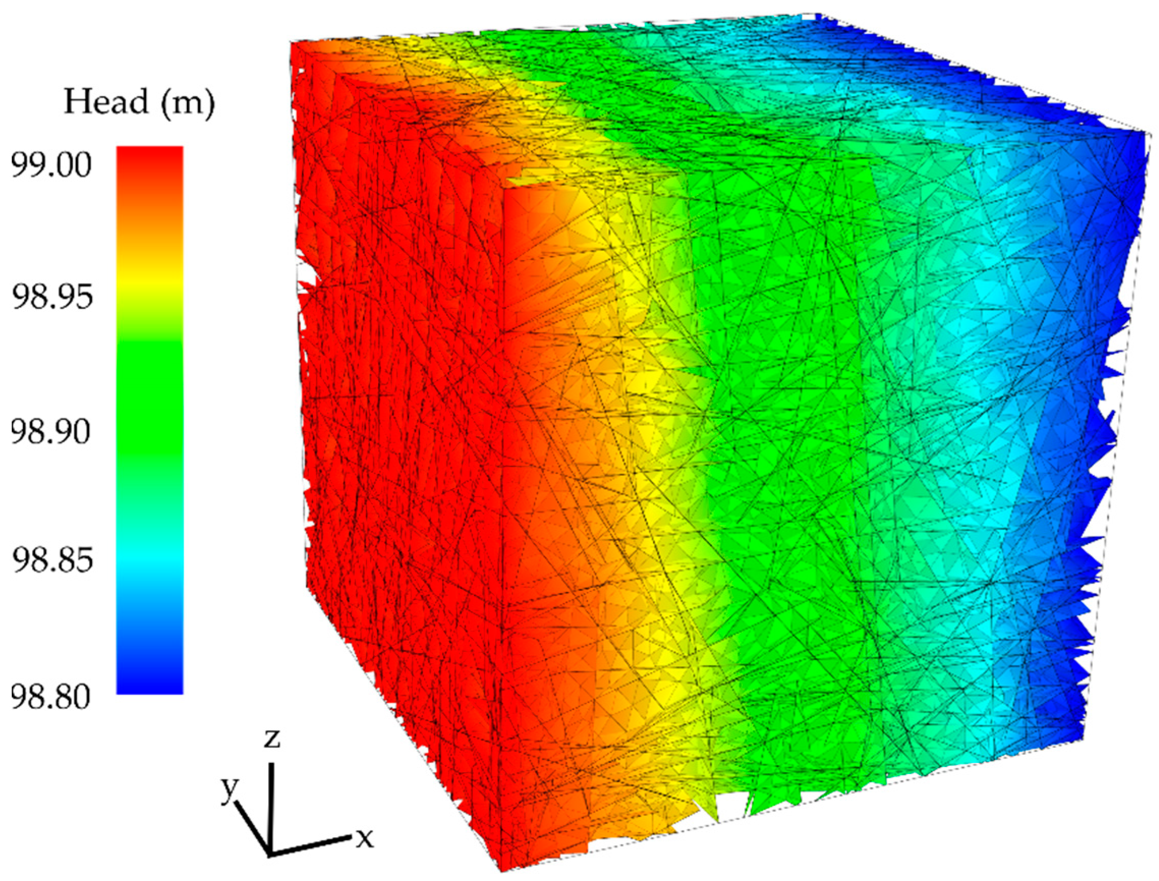
Case 2 and Case 3 share the same DFN realization that was generated based on the four fracture sets obtained from a selected site. Figure 8 shows the simulated flow field for a 100 × 100 × 100 m domain. The fracture intensities for the fracture sets were relativity high because of the shallow granite that might suffer strong weathering processes. The head gradient of 0.002 was designed to fit the regional groundwater head gradient near the site. The result in Figure 8 clearly shows that the hydraulic head in fractures varies from the west to the east boundaries. In Case 2 we released 100 particles from the high head boundary and placed the particles in the fractures that intersected with the upstream boundary. Case 3 used 100 particles, but the particles were randomly released along the well in the DFN. Note that we used a continuous source to simulate the contaminated well. There was no real water injection applied to the well. To simulate the reactive transport for the particle traces, we used the constant concentration of PCE for the PHREEQC simulations.
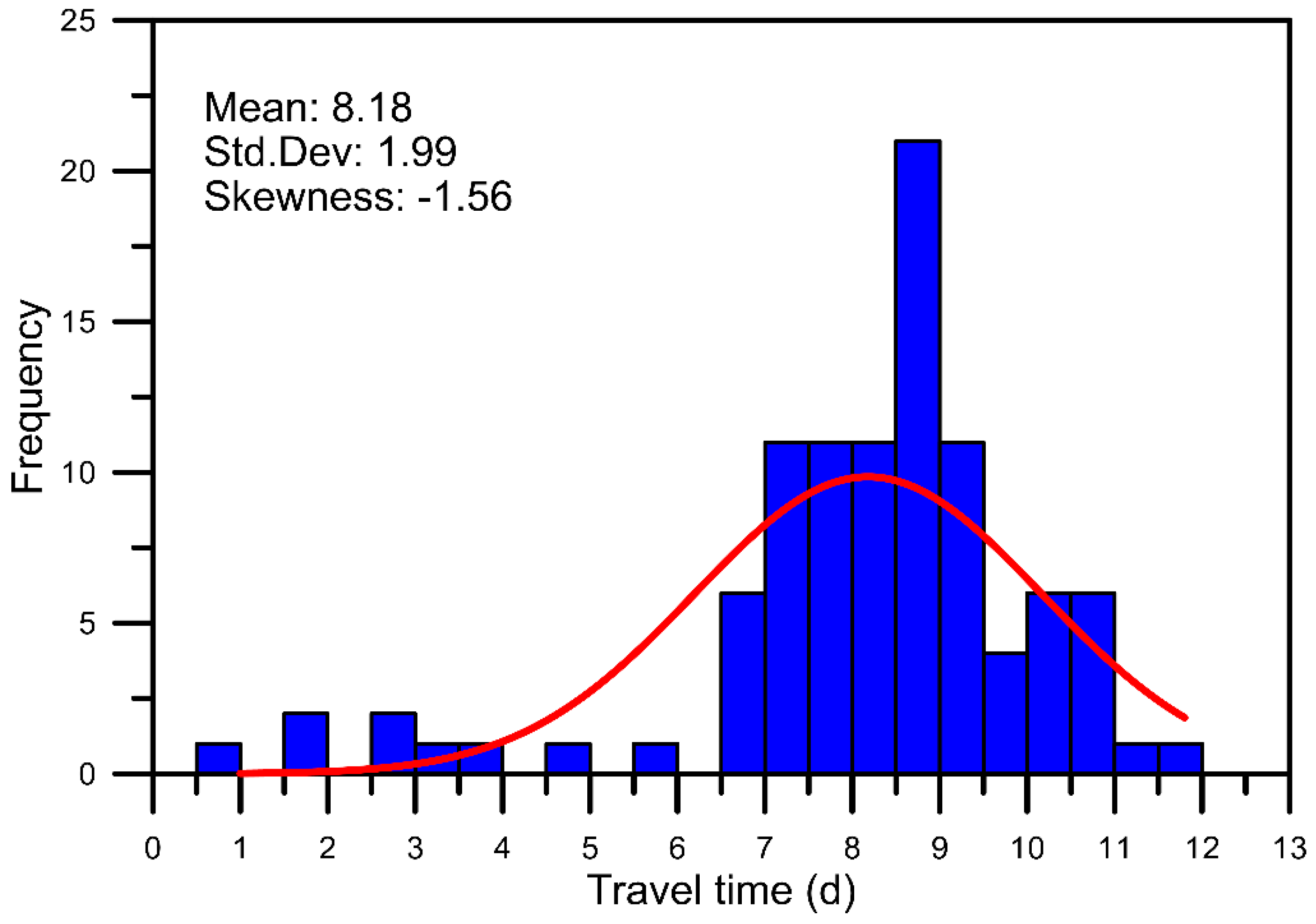
It is interesting to evaluate the overall behavior of traveling times obtained from PT simulations for different release scenarios in Cases 2 and 3. Figure 9 presents the histogram of travel times for the release of 100 particles in Case 2. The results for the line source particles in Case 3 are demonstrated in Figure 10. The results from the releasing scenarios show that the different release types can lead to different histogram distributions of traveling time. The line source in Case 3 shows a relatively small variation of particle travel time (see standard deviations in Figure 9 and Figure 10). As the release types and locations are different, Case 2 obtains a Skewed-left distribution with skewness index of −1.56, which indicates that few particles travel with short travel times, while most particles travel with longer travel times. On the other hand, the histogram for Case 3 shows that most particles released along the line source travel with relatively short times.
To quantify the influence of the specific fracture structure on the regional flow, the study further used 10 DFN realizations for Case 2 and conducted flow simulations for regional flows from the east to the west boundaries (i.e., constant heads specified on boundary faces x = 0 m and x = 100 m) and from the south to the north boundaries (i.e., constant heads specified on boundary faces y = 0 m and y = 100 m). The same regional head gradient of 0.002 was considered for the simulations. There are 100 particles randomly released on the upstream boundary faces (i.e., x = 0 m and y = 0 m) for the flow simulations. We collected the travel times of the released particles for the 10 DFN realizations. The histograms of the directional travel times are shown in Figure 11 for the x-direction flow and Figure 12 for the y-direction flow. Simulation results show that the mean travel time of the particles in the y-direction flow is larger than that in the x-direction flow. Additionally, the specified fracture sets (see Table 1) also induced a higher value of the travel time STD and led to a positive skewness in the y-direction flow. The inconsistent results of the travel time statistics indicate a clear anisotropic flow mechanism in the DFN flow (see parameters of fracture set 4 in Table 1). In the study, the fracture set 4 includes a number of high angle fractures and a high fracture intensity that are perpendicular to the y-direction flow. The direction barrier created by the fracture set 4 can be the factor that contributes to the inconsistency of the directional flows.
Comparing the statistics in Figure 9 and Figure 11 shows that the variation of the mean travel time is minor. However, considerable variations of travel time STD and skewness were obtained in two scenarios, indicating that the values of the travel time STD and skewness can be influenced by the number of DFN realizations. Based on the comparison of results from one, five, and 10 DFN realizations, we can obtain the stable values of the calculated travel time STD and skewness when we consider the number of DFN realizations greater than five. The critical number of the DFN realizations can produce representative values of travel time STD and skewness when the particle-based approaches were used for transport simulations. In most practical problems, the number of DFN realizations might depend on the behavior of a specified fracture structure. The relatively low fracture intensity might require more DFN realizations to obtain representative travel time statistics.
4.3. Propagation of Concentration Uncertainty
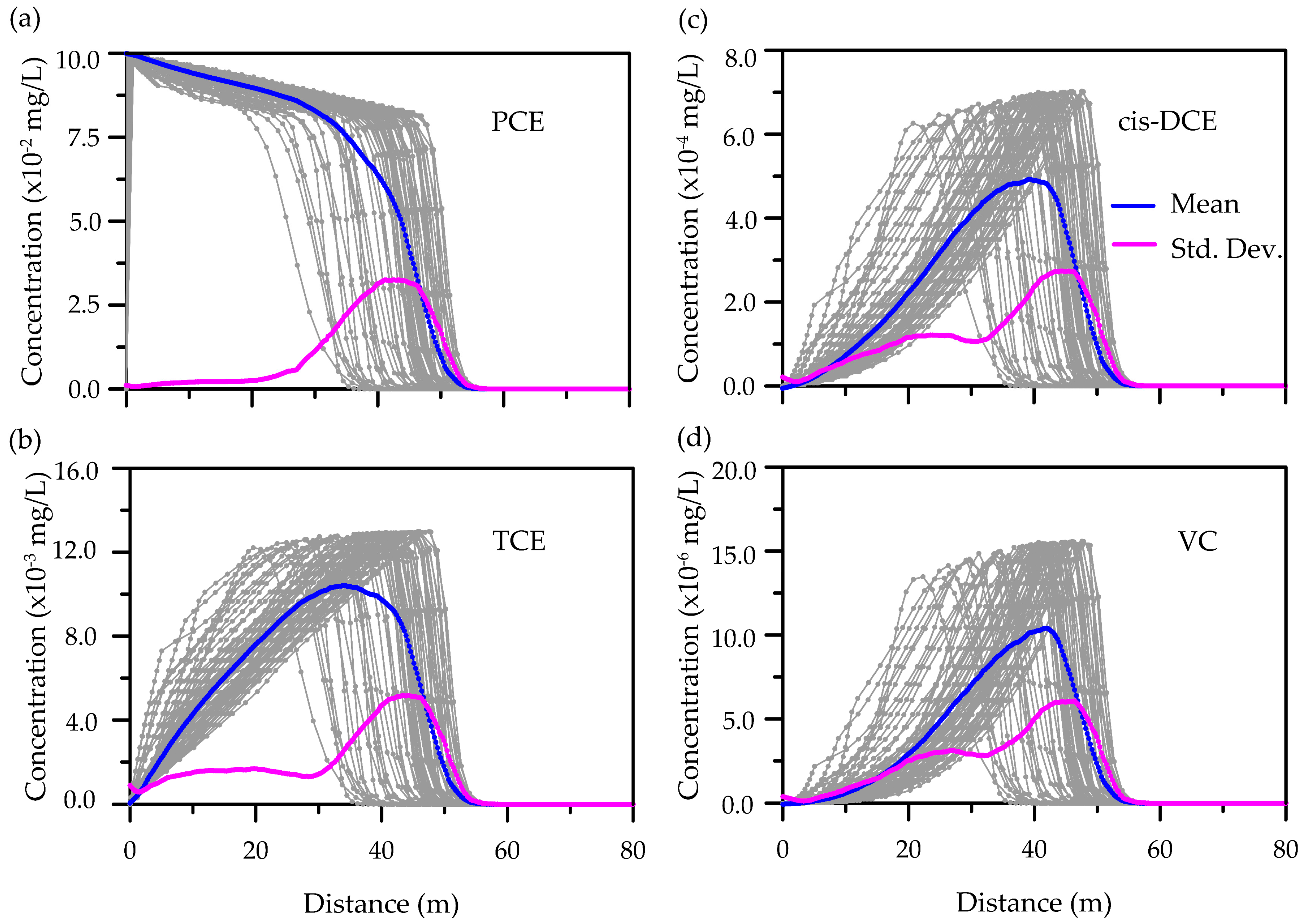
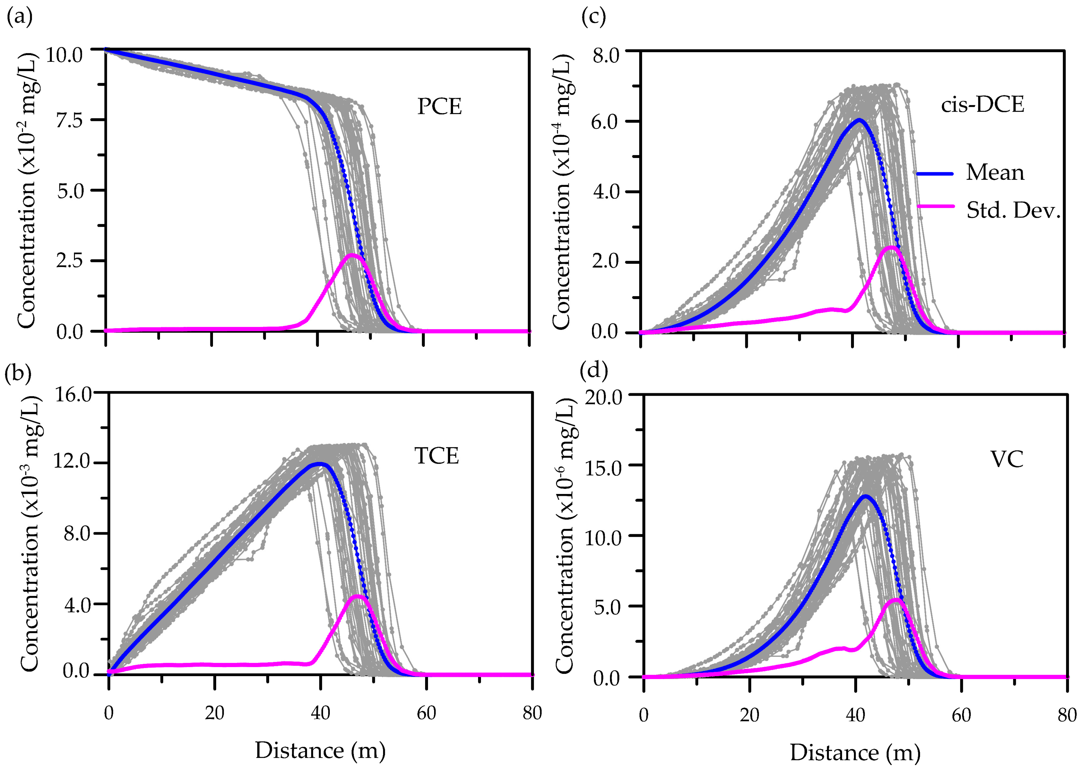
Figure 13 and Figure 14 show the collection of concentration along particle traces in Case 2 and Case 3. In these cases, we collected the concentration for the 100 particles and plotted the distribution of the concentration along the particle traces. Figure 13 and Figure 14 show the results for concentration at t = 3.0 days. The concentration along particle traces are plotted with the light color lines. Based on the collected concentration along the particle traces, Figure 13 and Figure 14 also show the values of means and STDs along the particle traces. For the specified time at t = 3.0 days, the estimated concentration uncertainty (i.e., STD) along the particle traces show high variation near the concentration fronts. The release scenario in Case 2 leads to the PCE concentration STD (i.e., MUP) reaching a maximal value of 0.3, while the release scenario in Case 3 shows the slightly small value of maximal STD for PCE concentration. Again, the concentration uncertainty can propagate to the daughter compounds such as the TCE, cis-DCE, or VC. The locations for the additional high uncertainty areas (i.e., SUPs) occur in the production zones of TCE, cis-DCE, and VC, where the concentration increases significantly. By comparing the uncertainty variations in Figure 13 and Figure 14, the results clearly show that the uncertainty influenced by the releasing scenario in Case 2 produces more uncertainty because the initial locations of the particles in Case 2 are randomly placed on a boundary face. However, the particle locations for Case 3 are limited along a line source at the well location.
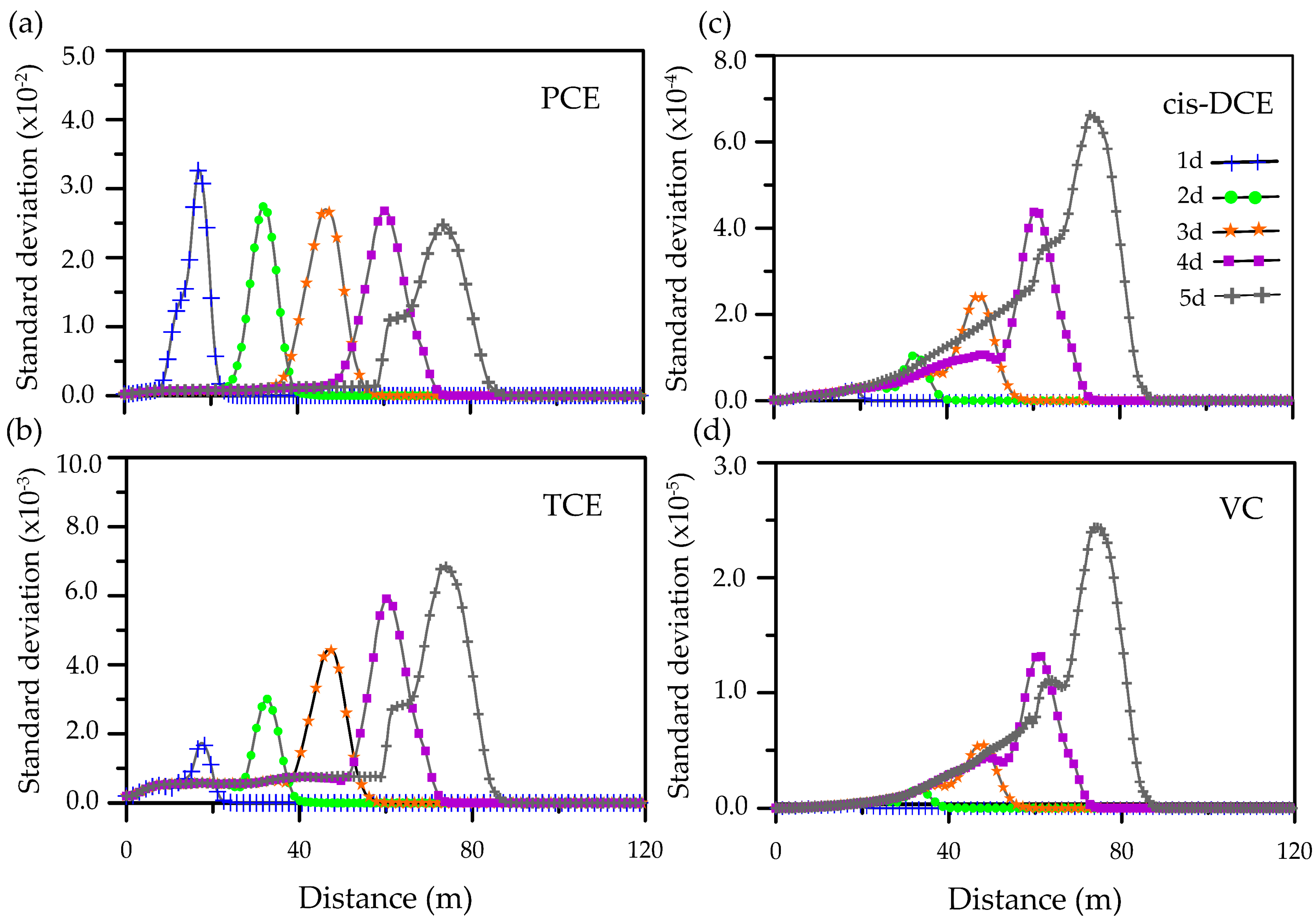
Figure 15 and Figure 16 further present the temporal variations of uncertainty for Cases 2 and 3. The simulation results show clear trends of uncertainty propagation under different releasing scenarios. In general, the uncertainty of PCE concentration gradually decreases with the traveling time and distance. However, the overall uncertainty (i.e., MUPs and SUPs) for the concentration of other daughter compounds increases with the traveling time and distance. We found that the uncertainty contributed from the parent compound PCE in each case increases with traveling time and distance. The SUPs produced by the daughter compounds also increase with the traveling time and distance. Ultimately, the SUPs in daughter compounds will mix with the MUPs for the late-time reactive transport (see Figure 15 and Figure 16). In this study, special cases were obtained in the variations of TCE concentration. The concentration in the production zones of TCE increases relatively linearly as compared with other daughter compounds. Therefore, the results show relatively stable values of SUP at different times.
4.4. Reactive Transport in the Complex 3D DFN
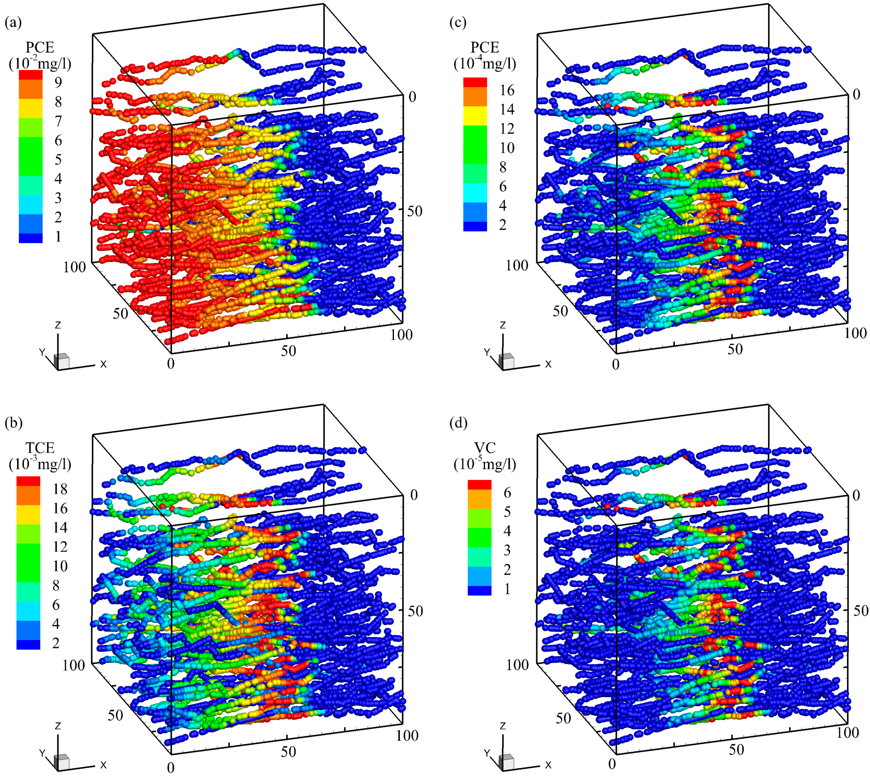
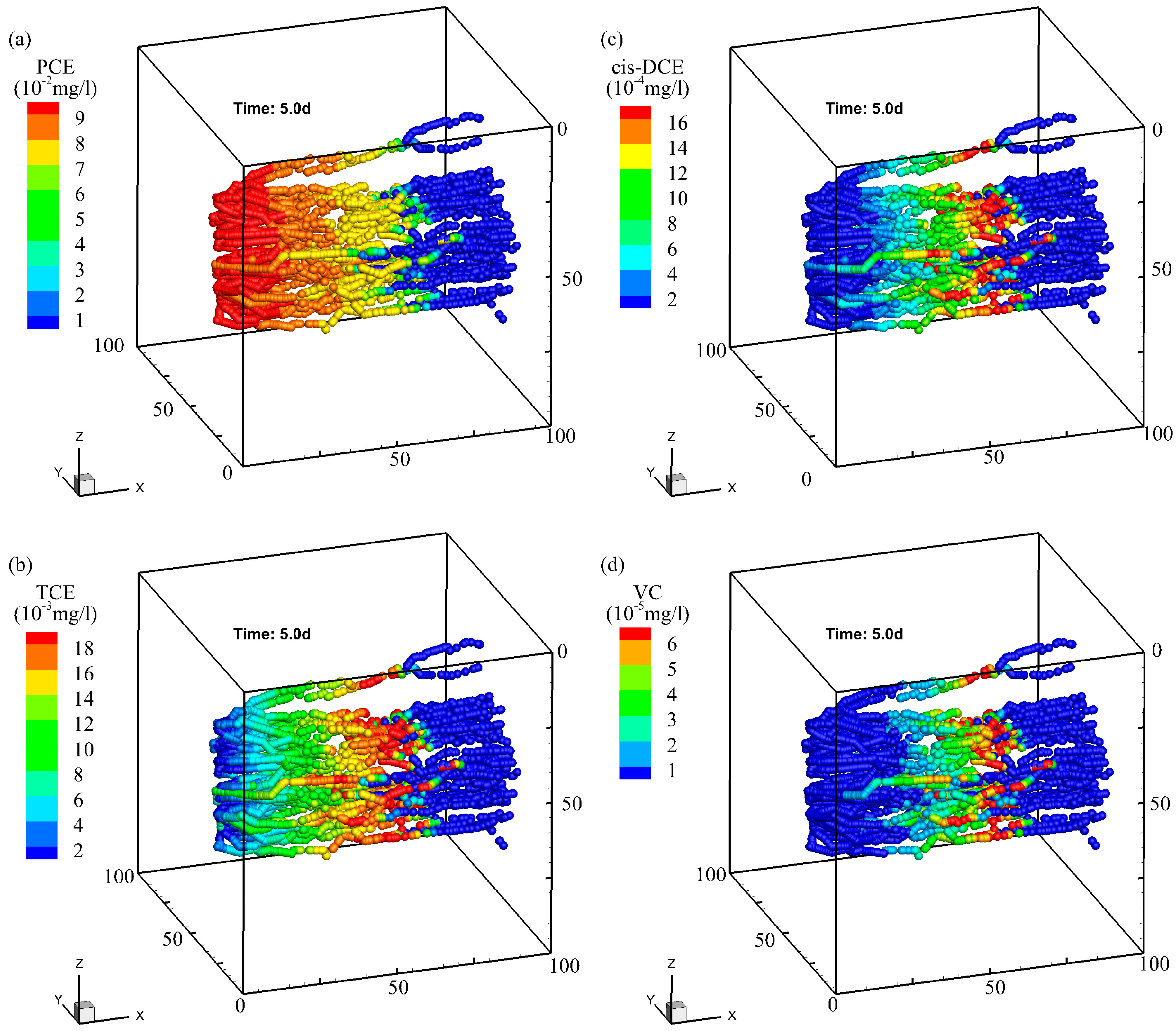
Hadgu et al. (2017) demonstrated the differences between the DFN and equivalent continuum models for simulating flow and transport in fractured rocks [50]. In this study, we assumed that the flow and transport are mainly controlled by the fracture networks. The workflow developed in this study aims to conduct simulations of tractive transport in complex 3D DFNs. In the workflow, the results of the PHREEQC simulations for particle traces were transformed back to the 3D coordinate system in the DFN. Figure 17 and Figure 18 show the concentration distribution for Cases 2 and Case 3 at t = 5.0 days. The results show that the high concentration of the daughter compounds occurs in the zones of the PCE concentration fronts. The results in Figure 17 and Figure 18 also show clear differences in the particle releasing types and the influences of the flow patterns in the DFN. In this study, the initial locations of particles have determined the concentration distributions in different cases. Case 2 shows a relatively random distribution of particle traces in the DFN domain. Therefore, the overall reactive transport presents in an average sense through the simulations. However, in Case 3 the particle locations were restricted along a line at a well location. The group of particle traces is also limited in a small area. Similar to the flow and transport in porous media, the small area can be defined as the well capture zone for the DFN flow. The capture zone is the key information to conduct remediation plans in fractured rock systems. For practical problems, the developed workflow can play an important role in assessing the transport procedures in DFNs and quantify the concentration for complex reactive transport. The implementations of other environmental issues are also feasible if the DFN recipes and the reaction parameters are available.
5. Conclusions
This study developed a computational workflow that enables the simulations of flow and tractive transport in complex 3D DFNs. The workflow successfully links a series of modeling procedures, including fracture generations, DFN flow modeling, particle tracking simulations, and reactive transport modeling. The procedures were available in the well-developed MAFIC and PHREEQC models. In the study, the linkage of data processing between models relies on the developed VBA script, which allows for preparing computational parameters for the PHREEQC modeling. The study illustrated the developed workflow with three numerical examples. Results indicated that the developed workflow is promising and can simulate flow and reactive transport for complex fracture connections.
The particle-based approach provides additional information for flow and reactive transport in the porous fractures. The travel time uncertainty of particles reflects the overall influences of particle releasing types and the fracture structure along the flow direction. The uncertainty of concentration also depends on the particle release types and the DFN structure. Uniform flow in the case with simple fracture connection yields a small variation of concentration, while the complex DFN results in relatively high variations of reactive transport. In this study, the simulations of the reactive transport obtained two clear peaks of concentration uncertainty. The parent compound PCEs mainly contribute to the development of MUPs and the MUPs can propagate from the parent to the daughter compounds. However, the production zones for daughter compounds might lead to a SUP. The influences of MUPs for daughter compounds can increase with the traveling time and distance. Ultimately, the MUPs from the parent compounds will mix with the SUPs for the late-time reactive transport.
A main challenge in the simulation workflow is to transform back the results of the PHREEQC model to the 3D DFN. Results in the study showed that the workflow enables the detailed visualization of reactive transport processes in complex 3D DFNs. In general, the high concentration of the daughter compounds occurs in the zones of the PCE concentration fronts. The different release types of particles considerably influence the flow patterns and transport behavior. For practical problems, the developed workflow can be a useful technique to assess and quantify the uncertainty of flow and reactive transport for site-specific scales and complexity. With the available reaction chains and rate constants, the workflow can be implemented for other environmental issues such as the geological storage of radionuclide waste and carbon dioxide.
6. Computer Code and Software
Software name: FracMan 7.51/MAFIC.
Developers: Golder Associates.
Contact information: https://www.golder.com/fracman/
Hardware required: 8 GB of RAM minimum (16 GB recommend), a minimum of 4 GB of free disk space, open GL compatible graphics card.
Software required: 32/64 bit: Windows 7 (or newer).
Program languages: PHREEQC and Visual Basic for Applications (VBA) in Microsoft Excel.
Availability: PHREEQC code follows User’s guide to PHREEQC (version 2) developed by USGS (https://pubs.er.usgs.gov/publication/wri994259). VBA program language is supported by Microsoft Excel. Output files of MAFIC simulations and VBA code can be obtained on GitHub at https://github.com/melinda93pthanh/Phreeqc/blob/master/VBAcode.
Author Contributions
C.-F.N. conceived the main idea of the paper. P.T.V. and C.-F.N. developed and tested the models. I.-H.L. and W.-C.L. prepared the figures. P.T.V., C.-F.N., W.-C.L., and C.-P.L. wrote the paper. All authors read and approved the final draft.
Funding
This research was partially supported by the Ministry of Science and Technology, Republic of China under grants MOST 107-2625-M-008-001, MOST 107-2116-M-008-003-MY2, MOST 108-2638-E-008-001-MY2, and by the Institute of Nuclear Energy Research, Atomic Energy Council, Executive Yuan under grant NL1030099.
Acknowledgments
We thank the anonymous reviewers for their constructive criticism and helpful comments.
Conflicts of Interest
The authors declare no conflict of interest.
References
- Lee, I.-H.; Ni, C.-F. Fracture-based modeling of complex flow and CO2 migration in three-dimensional fractured rocks. Comput. Geosci. 2015, 81, 64–77. [Google Scholar] [CrossRef]
- Baghbanan, A.; Jing, L. Hydraulic properties of fractured rock masses with correlated fracture length and aperture. Int. J. Rock Mech. Min. Sci. 2007, 44, 704–719. [Google Scholar] [CrossRef]
- Hyman, J.D.; Aldrich, G.; Viswanathan, H.; Makedonska, N.; Karra, S. Fracture size and transmissivity correlations: Implications for transport simulations in sparse three-dimensional discrete fracture networks following a truncated power law distribution of fracture size. Water Resour. Res. 2016, 52, 6472–6489. [Google Scholar] [CrossRef]
- Lee, I.-H.; Ni, C.-F.; Lin, F.-P.; Lin, C.-P.; Ke, C.-C. Stochastic modeling of flow and conservative transport in three-dimensional discrete fracture networks. Hydrol. Earth Syst. Sci. 2019, 23, 19–34. [Google Scholar] [CrossRef]
- Andersson, J.; Dverstorp, B. Conditional simulations of fluid flow in three-dimensional networks of discrete fractures. Water Resour. Res. 1987, 23, 1876–1886. [Google Scholar] [CrossRef]
- Dershowitz, W.; Miller, I. Dual porosity fracture flow and transport. Geophys. Res. Lett. 1995, 22, 1441–1444. [Google Scholar] [CrossRef]
- Painter, S.; Cvetkovic, V. Upscaling discrete fracture network simulations: An alternative to continuum transport models. Water Resour. Res. 2005, 41, 1029–2004. [Google Scholar] [CrossRef]
- Ni, C.-F.; Li, S.-G. Simple closed form formulas for predicting groundwater flow model uncertainty in complex, heterogeneous trending media. Water Resour. Res. 2005, 41. [Google Scholar] [CrossRef]
- Ni, C.-F.; Li, S.-G. Modeling groundwater velocity uncertainty in nonstationary composite porous media. Adv. Water Resour. 2006, 29, 1866–1875. [Google Scholar] [CrossRef]
- Ni, C.-F.; Li, S.-G.; Liu, C.-G.; Hsu, S.M. Efficient conceptual framework to quantify flow uncertainty in large-scale, highly nonstationary groundwater systems. J. Hydrol. 2009, 381, 297–307. [Google Scholar] [CrossRef]
- Long, J.C.S.; Gilmour, P.; Witherspoon, P.A. A model for steady fluid flow in random three-dimensional networks of discshaped fractures. Water Resour. Res. 1985, 21, 1105–1115. [Google Scholar] [CrossRef]
- Hyman, J.D.; Karra, S.; Makedonska, N.; Gable, C.W.; Painter, S.L.; Viswanathan, H.S. dfnWorks: A discrete fracture network framework for modeling subsurface flow and transport. Comput. Geosci. 2015, 84, 10–19. [Google Scholar] [CrossRef]
- de Dreuzy, J.-R.; Pichot, G.; Poirriez, B.; Erhel, J. Synthetic benchmark for modeling flow in 3D fractured media. Comput. Geosci. 2013, 50, 59–71. [Google Scholar] [CrossRef]
- Dreuzy, J.R.; Méheust, Y.; Pichot, G. Influence of fracture scale heterogeneity on the flow properties of three-dimensional discrete fracture networks (DFN). J. Geophys. Res. Solid Earth 2012, 117. [Google Scholar] [CrossRef]
- Xu, C.; Dowd, P. A new computer code for discrete fracture network modelling. Comput. Geosci. 2010, 36, 292–301. [Google Scholar] [CrossRef]
- Makedonska, N.; Painter, S.L.; Bui, Q.M.; Gable, C.W.; Karra, S. Particle tracking approach for transport in three-dimensional discrete fracture networks. Comput. Geosci. 2015, 19, 1123–1137. [Google Scholar] [CrossRef]
- Stalgorova, E.; Babadagli, T. Modified Random Walk–Particle Tracking method to model early time behavior of EOR and sequestration of CO2 in naturally fractured oil reservoirs. J. Pet. Sci. Eng. 2015, 127, 65–81. [Google Scholar] [CrossRef]
- Wang, L.; Cardenas, M.B.; Slottke, D.T.; Ketcham, R.A.; Sharp, J.M. Modification of the Local Cubic Law of fracture flow for weak inertia, tortuosity, and roughness. Water Resour. Res. 2015, 51, 2064–2080. [Google Scholar] [CrossRef]
- Painter, S.; Cvetkovic, V.; Mancillas, J.; Pensado, O. Time domain particle tracking methods for simulating transport with retention and first-order transformation. Water Resour. Res. 2008, 44. [Google Scholar] [CrossRef]
- Zafarani, A.; Detwiler, R.L. An efficient time-domain approach for simulating Pe-dependent transport through fracture intersections. Adv. Water Resour. 2013, 53, 198–207. [Google Scholar] [CrossRef]
- Park, Y.-J.; Lee, K.-K.; Kosakowski, G.; Berkowitz, B. Transport behavior in three-dimensional fracture intersections. Water Resour. Res. 2003, 39, 1215. [Google Scholar] [CrossRef]
- Xu, T.; Pruess, K. Modeling multiphase non-isothermal fluid flow and reactive geochemical transport in variably saturated fractured rocks: 1. Methodology. Am. J. Sci. 2001, 301, 16–33. [Google Scholar] [CrossRef]
- Steefel, C.I.; Appelo, C.A.J.; Arora, B.; Jacques, D.; Kalbacher, T.; Kolditz, O.; Lagneau, V.; Lichtner, P.C.; Mayer, K.U.; Meeussen, J.C.L.; et al. Reactive transport codes for subsurface environmental simulation. Comput. Geosci. 2015, 19, 445–478. [Google Scholar] [CrossRef]
- Deng, H.; Dai, Z.; Wolfsberg, A.; Lu, Z.; Ye, M.; Reimus, P. Upscaling of reactive mass transport in fractured rocks with multimodal reactive mineral facies. Water Resour. Res. 2010, 46. [Google Scholar] [CrossRef]
- Hunkeler, D.; Chollet, N.; Pittet, X.; Aravena, R.; Cherry, J.A.; Parker, B.L. Effect of source variability and transport processes on carbon isotope ratios of TCE and PCE in two sandy aquifers. J. Contam. Hydrol. 2004, 74, 265–282. [Google Scholar] [CrossRef]
- Kovacs, D.C.; Fischhoff, B.; Small, M.J. Perceptions of PCE use by dry cleaners and dry cleaning customers. J. Risk Res. 2001, 4, 353–375. [Google Scholar] [CrossRef]
- Ling, M.; Rifai, H.S. Modeling natural attenuation with source control at a chlorinated solvents dry cleaner site. Groundw. Monit. Remediat. 2007, 27, 108–121. [Google Scholar] [CrossRef]
- Conant, B., Jr.; Cherry, J.A.; Gillham, R.W. A PCE groundwater plume discharging to a river: Influence of the streambed and near-river zone on contaminant distributions. J. Contam. Hydrol. 2004, 73, 249–279. [Google Scholar] [CrossRef]
- Schaefer, C.E.; White, E.B.; Lavorgna, G.M.; Annable, M.D. Dense nonaqueous-phase liquid architecture in fractured bedrock: Implications for treatment and plume longevity. Environ. Sci. Technol. 2015, 50, 207–213. [Google Scholar] [CrossRef]
- Schaefer, C.E.; Callaghan, A.V.; King, J.D.; McCray, J.E. Dense nonaqueous phase liquid architecture and dissolution in discretely fractured sandstone blocks. Environ. Sci. Technol. 2009, 43, 1877–1883. [Google Scholar] [CrossRef]
- Delay, F.; Ackerer, P.; Danquigny, C. Simulating solute transport in porous or fractured formations using random walk particle tracking. Vadose Zone J. 2005, 4, 360–379. [Google Scholar] [CrossRef]
- Hyman, J.D.; Dentz, M.; Hagberg, A.; Kang, P.K. Linking structural and transport properties in three-dimensional fracture networks. J. Geophys. Res. Solid Earth 2019, 124. [Google Scholar] [CrossRef]
- Roubinet, D.; Liu, H.H.; de Dreuzy, J.R. A new particle-tracking approach to simulating transport in heterogeneous fractured porous media. Water Resour. Res. 2010, 46. [Google Scholar] [CrossRef] [Green Version]
- Tsang, Y.W.; Tsang, C.F. A particle-tracking method for advective transport in fractures with diffusion into finite matrix blocks. Water Resour. Res. 2001, 37, 831–835. [Google Scholar] [CrossRef]
- Viswanathan, H.S.; Hyman, J.D.; Karra, S.; O’Malley, D.; Srinivasan, S.; Hagberg, A.; Srinivasan, G. Advancing Graph-Based Algorithms for Predicting Flow and Transport in Fractured Rock. Water Resour. Res. 2018, 54, 6085–6099. [Google Scholar] [CrossRef]
- Sherman, T.; Hyman, J.D.; Bolster, D.; Makedonska, N.; Srinivasan, G. Characterizing the impact of particle behavior at fracture intersections in three-dimensional discrete fracture networks. Phys. Rev. E 2019, 99, 013110. [Google Scholar] [CrossRef] [Green Version]
- Parkhurst, D.L.; Appelo, C.A.J. User’s guide to PHREEQC (version 2)—A computer program for speciation, batch-reaction, one-dimensional transport, and inverse geochemical calculations. Water-Resour. Investig. Rep. 1999, 99, 312. [Google Scholar]
- Miller, I.; Lee, G.; Dershowitz, W. MAFIC–Matrix/Fracture Interaction Code with Heat and Solute Transport User Documentation, Version 2.0, Golder Associates; Redmond Inc.: Washington, DC, USA, 2001. [Google Scholar]
- Lei, Q.; Latham, J.-P.; Tsang, C.-F. The use of discrete fracture networks for modelling coupled geomechanical and hydrological behaviour of fractured rocks. Comput. Geotech. 2017, 85, 151–176. [Google Scholar] [CrossRef]
- La Pointe, P.R. A method to characterize fracture density and connectivity through fractal geometry. Int. J. Rock Mech. Min. Sci. Geomech. Abstr. 1988, 25, 421–429. [Google Scholar] [CrossRef]
- Hestir, K.; Long, J. Analytical expressions for the permeability of random two-dimensional Poisson fracture networks based on regular lattice percolation and equivalent media theories. J. Geophys. Res. Solid Earth 1990, 95, 21565–21581. [Google Scholar] [CrossRef] [Green Version]
- Davy, P.; Bour, O.; de Dreuzy, J.R.; Darcel, C. Flow in multiscale fractal fracture networks. Geol. Soc. Lond. Spec. Publ. 2006, 261, 31–45. [Google Scholar] [CrossRef]
- Fisher, N.I. Statistical Analysis of Circular Data; Cambridge University Press: Cambridge, UK, 1995. [Google Scholar]
- Mardia, K.V. Statistics of Directional Data; Academic Press: Cambridge, MA, USA, 1972. [Google Scholar]
- Kwicklis, E.M.; Healy, R.W. Numerical investigation of steady liquid water flow in a variably saturated fracture network. Water Resour. Res. 1993, 29, 4091–4102. [Google Scholar] [CrossRef]
- Pruess, K.; Tsang, Y.W. On two-phase relative permeability and capillary pressure of rough-walled rock fractures. Water Resour. Res. 1990, 26, 1915–1926. [Google Scholar] [CrossRef] [Green Version]
- Jacob, B. Dynamics of Fluids in Porous Media; American Elsevier Publishing Company: New York, NY, USA, 1972; pp. 579–663. [Google Scholar]
- Anderson, M.P.; Woessner, W.W.; Hunt, R.J. Applied Groundwater Modeling: Simulation of Flow and Advective Transport, 2nd ed.; Academic Press: Cambridge, MA, USA, 2015. [Google Scholar]
- Jacques, D.; Šimůnek, J. User Manual of the Multicomponent Saturated Transport Model HP1: Discription, Verification and Examples; BLG-998; SCK.CEN: Mol, Belgium, 2004. [Google Scholar]
- Hadgu, T.; Karra, S.; Kalinina, E.; Makedonska, N.; Hyman, J.D.; Klise, K.; Viswanathan, H.S.; Wang, Y. A comparative study of discrete fracture network and equivalent continuum models for simulating flow and transport in the far field of a hypothetical nuclear waste repository in crystalline host rock. J. Hydrol. 2017, 553, 59–70. [Google Scholar] [CrossRef]
Figure 1.
The concept and the main steps involved in the workflow in the study.

Figure 2.
The concept of procedures for particle tracking (PT) and PHREEQC simulations.

Figure 3.
The conceptual model and the fracture networks for simulation of reactive transport in this study: (a) Case 1 with the simple connection of three fractures, (b) Case 2 and Case 3 with a complex discrete fracture network (DFN) realization that is generated based on fracture sets obtained from the selected site.

Figure 4.
The degradation pathways of tetrachloroethylene (PCE) using first-order rate constants [49].
Figure 4.
The degradation pathways of tetrachloroethylene (PCE) using first-order rate constants [49].

Figure 5.
The results for flow and reactive transport simulations along a selected particle trace: (a) the head distribution for the simple fracture connection, (b) the distribution of PCE concentration along the selected particle trace, and (c) the associated daughter compounds trichloroethylene (TCE), (d) cis-1,2-dichloroethylene (cis-DCE), and (e) vinyl chloride (VC).

Figure 6.
The concentration distribution at t = 1.0 day for 50 particle traces and the calculated uncertainty distributions for (a) PCE, (b) cis-DCE, (c) TCE, and (d) VC.
Figure 6.
The concentration distribution at t = 1.0 day for 50 particle traces and the calculated uncertainty distributions for (a) PCE, (b) cis-DCE, (c) TCE, and (d) VC.

Figure 7.
The distributions of different concentration at t = 1.5 days in Case 1: (a) PCE, (b) TCE, (c) cis-DCE, and (d) VC.
Figure 7.
The distributions of different concentration at t = 1.5 days in Case 1: (a) PCE, (b) TCE, (c) cis-DCE, and (d) VC.

Figure 8.
Distribution of hydraulic head for the generated DFN.

Figure 9.
The histogram of travel times for the 100 particles in Case 2.

Figure 10.
The histogram of travel times for the 100 particles in Case 3.

Figure 11.
Histogram of travel time for x-direction flow.

Figure 12.
Histogram of travel time for y-direction flow.

Figure 13.
The PT concentration for Case 2 at t = 3.0 days: (a) PCE, (b) TCE, (c) cis-DCE, and (d) VC.
Figure 13.
The PT concentration for Case 2 at t = 3.0 days: (a) PCE, (b) TCE, (c) cis-DCE, and (d) VC.

Figure 14.
The PT concentration for Case 3 at t = 3.0 days: (a) PCE, (b) TCE, (c) cis-DCE, and (d) VC.
Figure 14.
The PT concentration for Case 3 at t = 3.0 days: (a) PCE, (b) TCE, (c) cis-DCE, and (d) VC.

Figure 15.
The propagation of concentration uncertainty for different times in Case 2, (a) PCE, (b) TCE, (c) cis-DCE, and (d) VC.
Figure 15.
The propagation of concentration uncertainty for different times in Case 2, (a) PCE, (b) TCE, (c) cis-DCE, and (d) VC.

Figure 16.
The propagation of concentration uncertainty for different times in Case 3, (a) PCE, (b) TCE, (c) cis-DCE, and (d) VC.
Figure 16.
The propagation of concentration uncertainty for different times in Case 3, (a) PCE, (b) TCE, (c) cis-DCE, and (d) VC.

Figure 17.
The 3D concentration distribution for Case 2 at time t = 5 days: (a) PCE, (b) TCE, (c) cis-DCE, and (d) VC.
Figure 17.
The 3D concentration distribution for Case 2 at time t = 5 days: (a) PCE, (b) TCE, (c) cis-DCE, and (d) VC.

Figure 18.
The 3D concentration distribution for Case 3 at time t = 5.0 days: (a) PCE, (b) TCE, (c) cis-DCE, and (d) VC.
Figure 18.
The 3D concentration distribution for Case 3 at time t = 5.0 days: (a) PCE, (b) TCE, (c) cis-DCE, and (d) VC.


Table 1.
The fracture parameters and hydrogeological conditions for simulation cases. Notation T is the mean trend and P is the mean plunge. The Fisher constant k and fracture intensity P32 are used for generating the complex DFN for Case 2 and Case 3.
Table 1.
The fracture parameters and hydrogeological conditions for simulation cases. Notation T is the mean trend and P is the mean plunge. The Fisher constant k and fracture intensity P32 are used for generating the complex DFN for Case 2 and Case 3.
| Network | Fracture Orientation | Aperture (m) | Transmissivity (m2/s) | Hydraulic Gradient | ||||
|---|---|---|---|---|---|---|---|---|
| T | P | k | P32 | |||||
| Case 1 | Fracture 1 | 0 | 90 | - | - | 1 × 10⁻⁴ | 1 × 10⁻⁴ | 0.0025 |
| Fracture 2 | 0 | 0 | - | - | ||||
| Fracture 3 | 0 | 90 | - | - | ||||
| Case 2 and Case 3 | Set 1 | 198 | 18 | 18 | 0.26 | 1 × 10⁻⁴ | 1 × 10⁻⁵ | 0.002 |
| Set 2 | 155 | 4 | 15 | 0.24 | ||||
| Set 3 | 264 | 23 | 16 | 0.18 | ||||
| Set 4 | 98 | 91 | 11 | 0.32 | ||||
Table 2.
The computational parameters for PHREEQC transport models.
| Parameters | Value | Units |
|---|---|---|
| Initial concentration | 0 | - |
| Source concentration | 0.1 | mg/L |
| Cells | Variable | - |
| Shifts | Variable | - |
| Time step | 846 (for Case 1) | s |
| 8460 (for Case 2 and Case 3) | s | |
| Dispersion coefficient | 0.5 (for Case 1) | m2/s |
| 0.05 (for Case 2 and Case 3) | m2/s |
Table 3.
The parameters for the PCE biodegradation in the study [49].
Table 3.
The parameters for the PCE biodegradation in the study [49].
| Parameter | Symbol | Value | Unit |
|---|---|---|---|
| First-order degradation rate 1 | k1 | 0.075 | d−1 |
| First-order degradation rate 2 | k2 | 0.070 | d−1 |
| First-order degradation rate 3 | k3 | 0.020 | d−1 |
| First-order degradation rate 4 | k4 | 0.035 | d−1 |
| First-order degradation rate 5 | k5 | 0.055 | d−1 |
| First-order degradation rate 6 | k6 | 0.030 | d−1 |
| Distribution factor, TCE to cis-DCE | α1 | 0.72 | - |
| Distribution factor, TCE to trans-DCE | α2 | 0.15 | - |
| Distribution factor, TCE to 1,1-DCE | α3 | 0.13 | - |
| Yield coefficient, PCE to TCE | γ1 | 0.79 | - |
| Yield coefficient, TCE to DCE | γ2 | 0.74 | - |
| Yield coefficient, DCE to VC | γ3 | 0.64 | - |
| Yield coefficient, VC to ETH | γ4 | 0.45 | - |
© 2019 by the authors. Licensee MDPI, Basel, Switzerland. This article is an open access article distributed under the terms and conditions of the Creative Commons Attribution (CC BY) license (http://creativecommons.org/licenses/by/4.0/).
Share and Cite
MDPI and ACS Style
Vu, P.T.; Ni, C.-F.; Li, W.-C.; Lee, I.-H.; Lin, C.-P. Particle-Based Workflow for Modeling Uncertainty of Reactive Transport in 3D Discrete Fracture Networks. Water 2019, 11, 2502. https://doi.org/10.3390/w11122502
AMA Style
Vu PT, Ni C-F, Li W-C, Lee I-H, Lin C-P. Particle-Based Workflow for Modeling Uncertainty of Reactive Transport in 3D Discrete Fracture Networks. Water. 2019; 11(12):2502. https://doi.org/10.3390/w11122502
Chicago/Turabian StyleVu, Phuong Thanh, Chuen-Fa Ni, Wei-Ci Li, I-Hsien Lee, and Chi-Ping Lin. 2019. "Particle-Based Workflow for Modeling Uncertainty of Reactive Transport in 3D Discrete Fracture Networks" Water 11, no. 12: 2502. https://doi.org/10.3390/w11122502
Note that from the first issue of 2016, this journal uses article numbers instead of page numbers. See further details here.