A Methodology for the Fast Comparison of Streamwater Diurnal Cycles at Two Monitoring Points


1
Department of Geography, Ștefan cel Mare University of Suceava, Universității 13, 720229 Suceava, Romania
2
Computers, Electronics and Automation Department, Ștefan cel Mare University of Suceava, Universității 13, 720229 Suceava, Romania
*
Author to whom correspondence should be addressed.
Water 2019, 11(12), 2524; https://doi.org/10.3390/w11122524
Submission received: 23 October 2019
/
Revised: 25 November 2019
/
Accepted: 27 November 2019
/
Published: 29 November 2019
(This article belongs to the Special Issue Impacts of Anthropogenic Activities on Watersheds in a Changing Climate)
Abstract
:There are numerous streamwater parameters that exhibit a diurnal cycle. However, the shape of this cycle has a huge variation from one parameter to another and from one monitoring point to another on the same river. Important variations also occur at the same point during some events, such as high waters. Water level, specific conductivity, dissolved oxygen, oxidation reduction potential, and pH of the Suceava River were monitored for 365 days (2018–2019, hourly sampling frequency) in order to assess the upstream-downstream changes in the diurnal cycle of these parameters, some of these changes being caused by the impact of Suceava city, which is located between the selected monitoring points. The multiresolution analysis of the maximal overlap discrete wavelet transform and the wavelet coherence analysis were combined in a flexible methodology that helped in comparing the upstream and downstream shapes of the diurnal cycle. The methodology allowed for a fast comparison of diurnal profiles during periods of high waters or baseflow. Notable changes were observed in the moments of diurnal maxima and minima.
1. Introduction
The wavelet analysis of streamwater parameters has become more and more popular in the last two decades due to the advantages of this method for the study of non-linear processes [1,2]. Wavelet analysis techniques were applied mostly on stage or discharge time series due to the wide availability of this type of data [3]. It is in the last decade when water quality parameters were involved intensively in wavelet analyses [4,5]. Some physical and chemical properties of streamwaters are proper indicators of water quality and can be used to trace the environmental impact of man. The specific conductivity, dissolved oxygen, oxidation reduction potential (ORP), and pH of a river water can be used to indicate the impact of urban areas on the environment and are sometimes included in wavelet analyses [5,6,7]. Cities modify the properties of natural waters through various active or passive processes, such as the discharge of stormwater runoff or the creation of an urban heat island, which has multiple effects on urban waters [8]. Urban wastewater treatment plants can alter the diurnal profile of a streamwater chemistry parameter [9,10].
The diurnal cycle in streamwaters is caused by the Earth’s rotation around its axis, which leads to the day/night cycle. This cycle modifies evaporation and evapotranspiration in catchments [11,12]. These changes can be measured as variations in the temporal evolution of numerous streamwater parameters, which often have an interdependent behavior with the diurnal oscillation [13]. Natural or anthropogenic events (such as rainfall or pollution events) add transient fluctuations in the diurnal cycle. Finding a relevant shape of the diurnal cycle is needed in order to distinguish the periodic and aperiodic modifications in case study time series. A high resolution diurnal profile is obtained from high frequency measurements. This is why, up-to-date, such profiles are missing in Romania for most water quality parameters. Existing studies on diurnal streamwater profiles have focused on water level or water temperature [10,14].
Streamwater monitoring in Romania is done mainly by the Romanian Waters National Administration, whose data is sometimes used in studies about water chemistry of the Suceava River [15], but this data lacks high frequency sampling and the needed spatial density along a river. The environmental impact of some water contaminants is often assessed for various areas in Romania [16,17,18,19,20] and cities have a traceable impact on streamwater quality [21].
A monitoring system that measures Suceava River water quality upstream and downstream of Suceava city was implemented in 2018 and this study aimed to provide a methodology for a fast analysis of the diurnal cycles of various streamwater parameters at two monitoring points. The wavelet analysis was used to reveal the spatial and temporal variations in the streamwater diurnal cycles. The speedier analysis is needed for the growing sizes of databases. It is often useful to apply an analysis method that acts as an easily adjustable preview of data in order to identify interesting phenomena for further analyses. Also, to our knowledge, this was the first study that computes the average diurnal profiles of specific conductivity, dissolved oxygen, ORP, and pH for the Suceava River.
The methodology proposed in this study was applied to streamwater data from monitoring points located above and below a city in order to discover some details of how the diurnal profile of a river is affected by a city. In this paper, we indicate some links between the observed variations in diurnal profiles and urban elements, such as the urban wastewaters or the urban heat island, that generate the environmental impact of a city.
2. Materials and Methods
2.1. Study Area
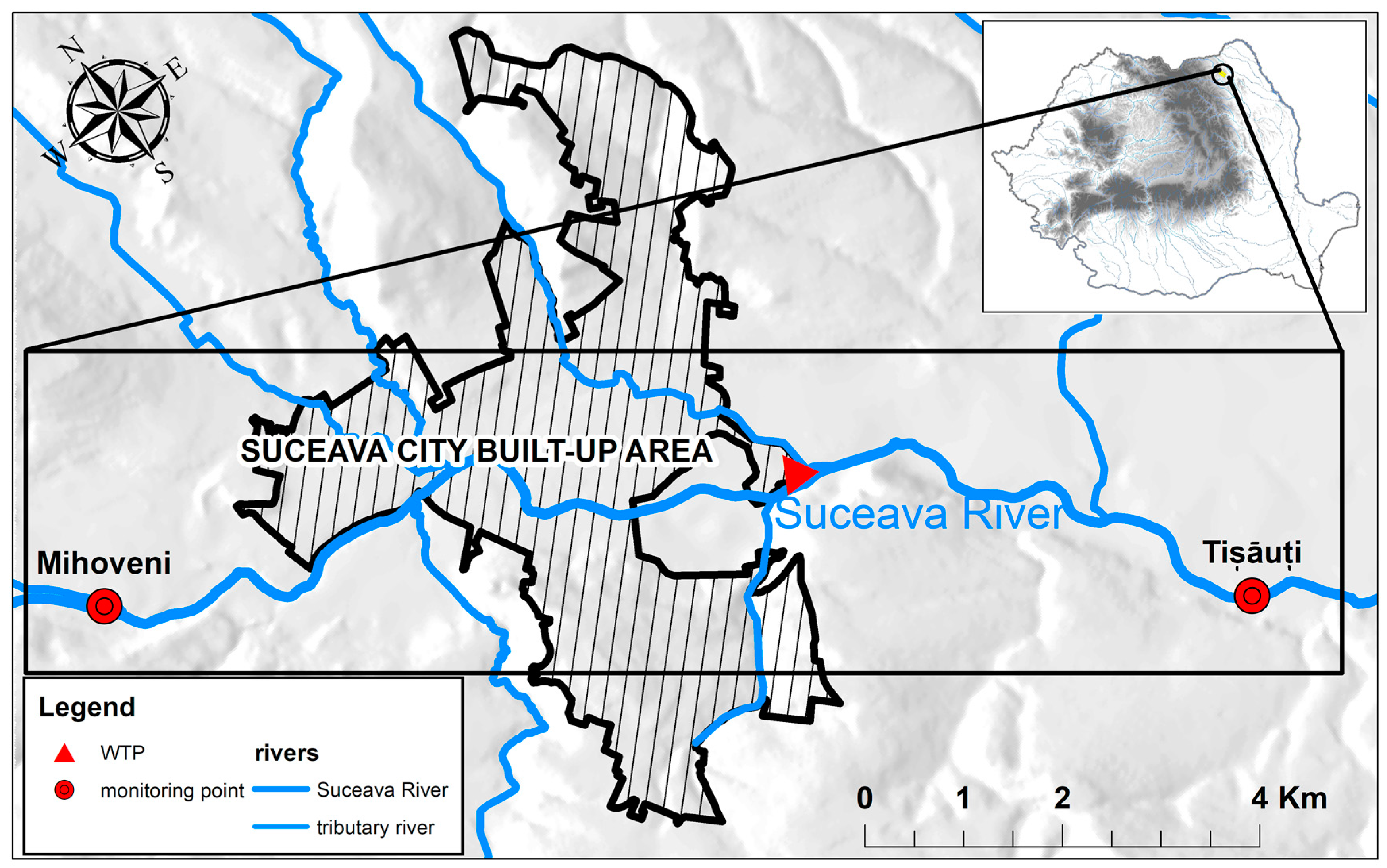
The monitoring system. which provided data in this study, was implemented by the University of Suceava and consisted of two monitoring points where water properties are measured every hour (the monitoring points are 11.6 km in a straight line away from each other, with Suceava city in the middle of this distance). Suceava city has a total number of inhabitants fluctuating around 100,000 people.
The study area was located in Suceava Plateau, part of the Moldavian Plateau. Climate is temperate continental with warm and wet summers (the average annual air temperature is 7.86 °C and the annual sum of precipitation is 578 mm [10]). The streambed elevation between the selected points ranged approximately from 280 to 260 m above sea level (a.s.l.) and has a sinuous path, which helps in mixing streamwater so that it records identical values at any point of a transversal section. The upstream monitoring point was at Mihoveni Dam (47.681° N, 26.2° E). This is a quasi-inactive dam aimed at generating run-of-the-river hydroelectricity; it operates only during some high water events for regulating the water level. The downstream monitoring point was placed at Tișăuți (47.618° N, 26.323° E), downstream of an urban wastewater treatment plant and some floodplain landfills (Figure 1). The Suceava River has an average flow rate of 16.87 m3/s inside Suceava City [10]. The Suceava River has two periods of high waters. The first one occurs during the middle of springtime (April, monthly average flow rate of 29.7 m3/s) due to snowmelt in the catchment, especially in the mountain area, while the second one happens at the beginning of summer (June, 29.9 m3/s) as result of heavy rainfalls [10]. During high water events, the Suceava River frequently exceeds 50 m3/s. The lowest monthly average flow rate is recorded during the winter (January, 6.2 m3/s) because of the negative air temperatures and little precipitation [10]. The urban tributaries of the Suceava River in the study area had a total discharge of approximately 0.5 m3/s. The water chemistry of rivers in north-eastern Romania, which includes our study area, was briefly discussed in some studies [22,23], some of them highlighting the intense self-purification processes of Suceava River water inside and downstream of the city [24]. However, these studies were not based on long time series with high frequency of measurements.
2.2. Instruments
Two AquaTROLL 500 multiparameter probes were used to monitor physical and chemical streamwater properties (paired with two Tube 300R for telemetry). The instruments were equipped with sensors that measured: pressure/level (accuracy: ±0.1% full scale (9 m), resolution: 0.01% full scale), electrical conductivity (automatically converted to specific conductivity (SC); accuracy: ±0.5% of reading +1 μS/cm, resolution: 0.1 μS/cm), dissolved oxygen (DO; accuracy: ±0.1 mg/L, resolution: 0.01 mg/L), oxidation reduction potential (ORP; accuracy: ±5 mV, resolution: 0.1 mV), and pH (accuracy: ± 0.1 pH unit, resolution: 0.01 pH).
2.3. Data
Data analyzed in this study were recorded from 10 October 2018 until 9 October 2019 (with one exception: DO data is missing from November 7 to December 5, 2018). The local standard time (EET) was used for all time series. Corrections were applied to our data as follows: compensations were applied after periodic instrument calibrations, missing singular values were obtained by using linear interpolation, outliers were removed through replacement with values from data smoothed with a moving average filter, and some missing consecutive values were obtained by using regression equations. At the downstream sampling point, the measurements were sometimes affected by residuals from wastewaters and the time series were verified by using independent measurements carried out using a Hach HQ40d portable multiparameter instrument. Data of all parameters can be viewed and downloaded at the project website, http://water.usv.ro/data.php (where a map of the study area can also be inspected).
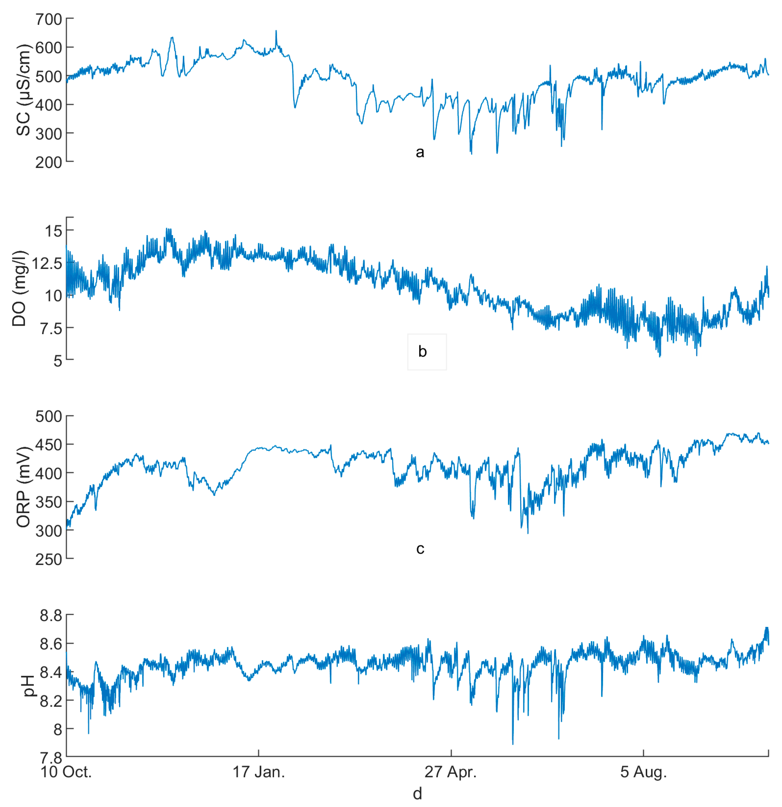
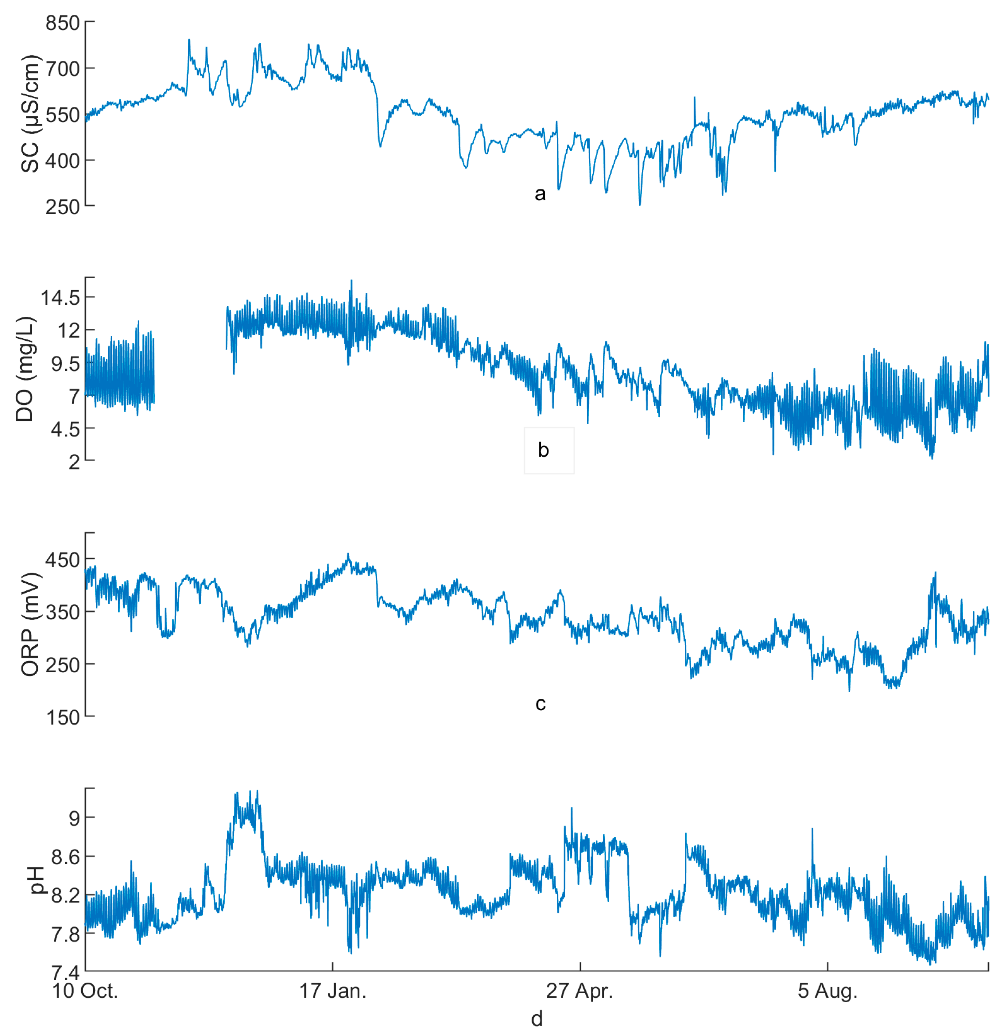
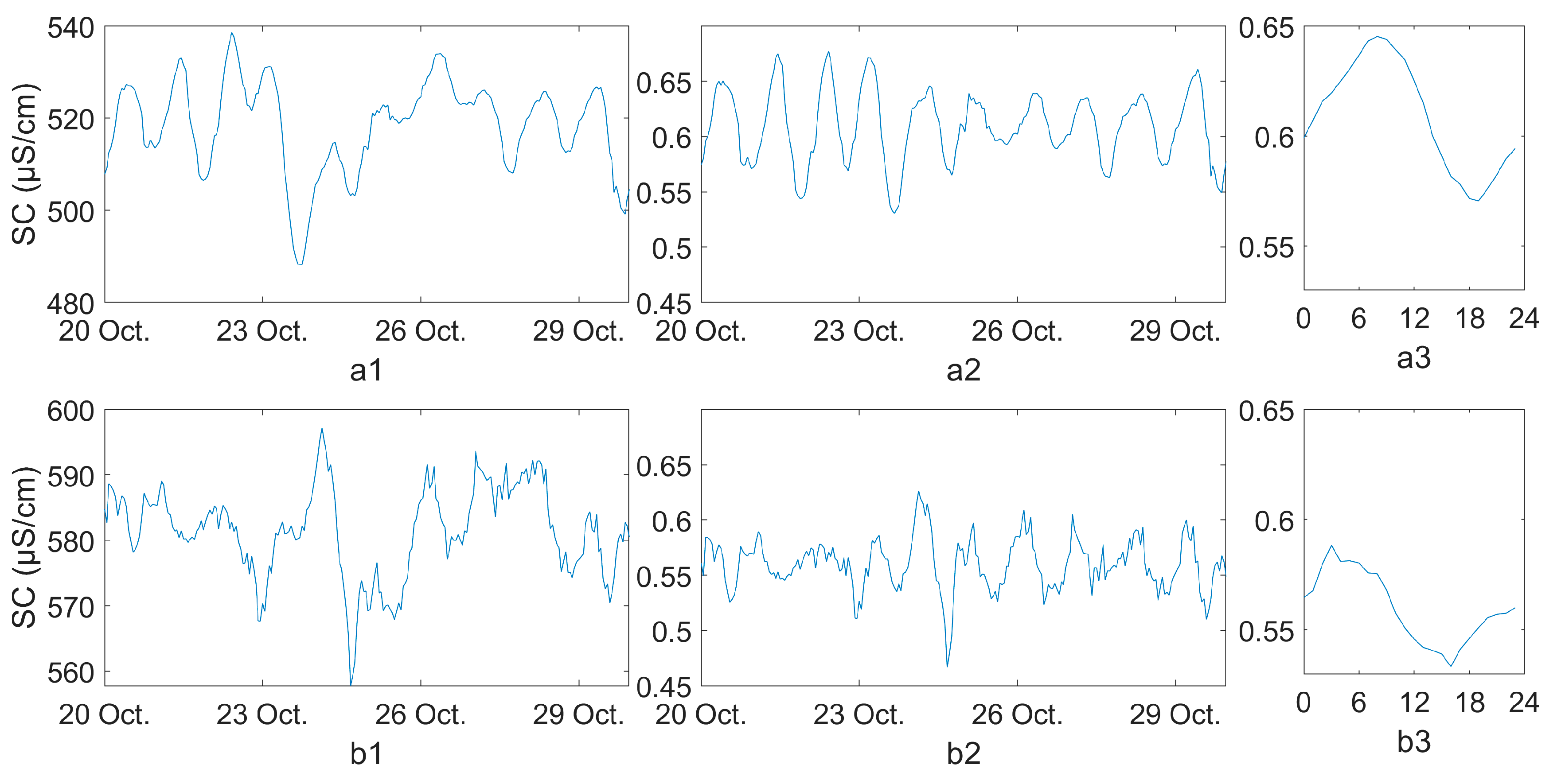
The yearly average of the specific conductivity was higher downstream (at Tișăuți; 549 µS/cm) than upstream (at Mihoveni; 483.1 µS/cm) and the standard deviation values had the same relationship (97.9 µS/cm versus 72.4 µS/cm). Urban wastewaters were the main cause of the differences; treated and untreated waters are discharged into the Suceava River through the wastewater treatment plant effluent and Cetății Creek [10,23,25]. The difference is much larger after snowfalls, when de-icing measures are applied and/or when high air temperatures lead to important snowmelt and runoff from roads and roofs (see, for example, peaks in SC that were only recorded in the second half of November 2018 downstream after large snowfalls occurred) (Figure 2 and Figure 3). Dissolved oxygen had mean values of 10.6 and 8.82 mg/L (upstream and downstream, with corresponding standard deviations of 2.06 and 2.69 mg/L, respectively). The lower average value downstream of the urban areas was an effect of a warmer and more polluted streamwater. The urban heat island was observed in the study area in a previous study [10].
ORP mean values upstream and downstream were 412.16 and 338.01 mV and standard deviation at these points was 32.11 and 52.97 mV, respectively. The values of pH were 8.45 (upstream) and 8.22 (downstream) and the difference in standard deviations was the greatest of all parameters: 0.09 (upstream) and 0.31 (downstream).
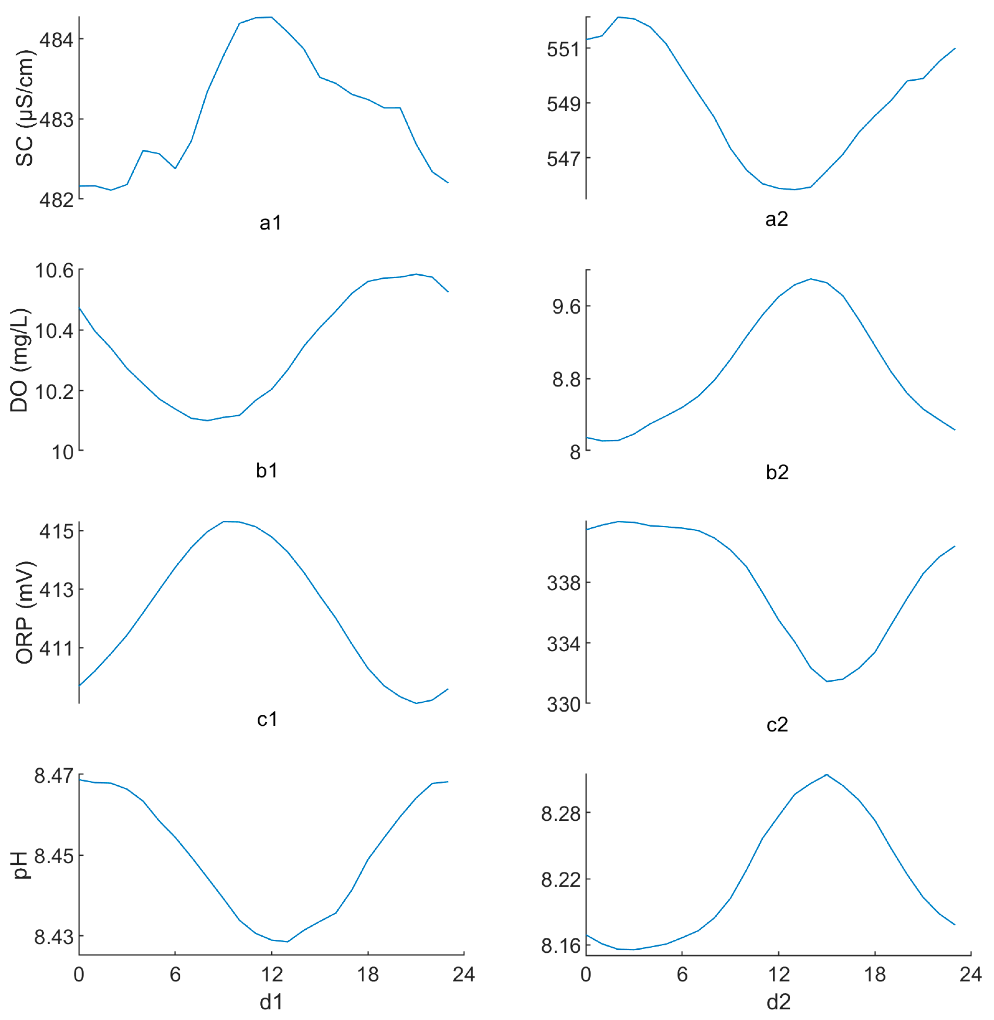
The average diurnal profiles of SC, DO, ORP, and pH indicated differences in the shapes and positions of the diurnal maxima and minima not only between parameters, but also between the values of the same parameter at the two monitoring points (Figure 4). SC upstream had a diurnal maximum during midday (11:00–12:00), while downstream, the maximum was recorded at 03:00. The maximum values of DO recorded were in the late afternoon and early evening at the selected monitoring points; this difference was not caused by the streamwater temperature, which had similar moments of maxima in the study area [10]. Rather, this similarity happens instead of an inverse relationship that should occur theoretically. The average hourly values of downstream ORP created a prolonged interval with maximum values in the first third of the day. The diurnal minimum of upstream pH occurred at 13:00 and might be partly explained by the theoretical inverse relationship between pH and temperature, but the downstream pH maxima was recorded at 15:00.
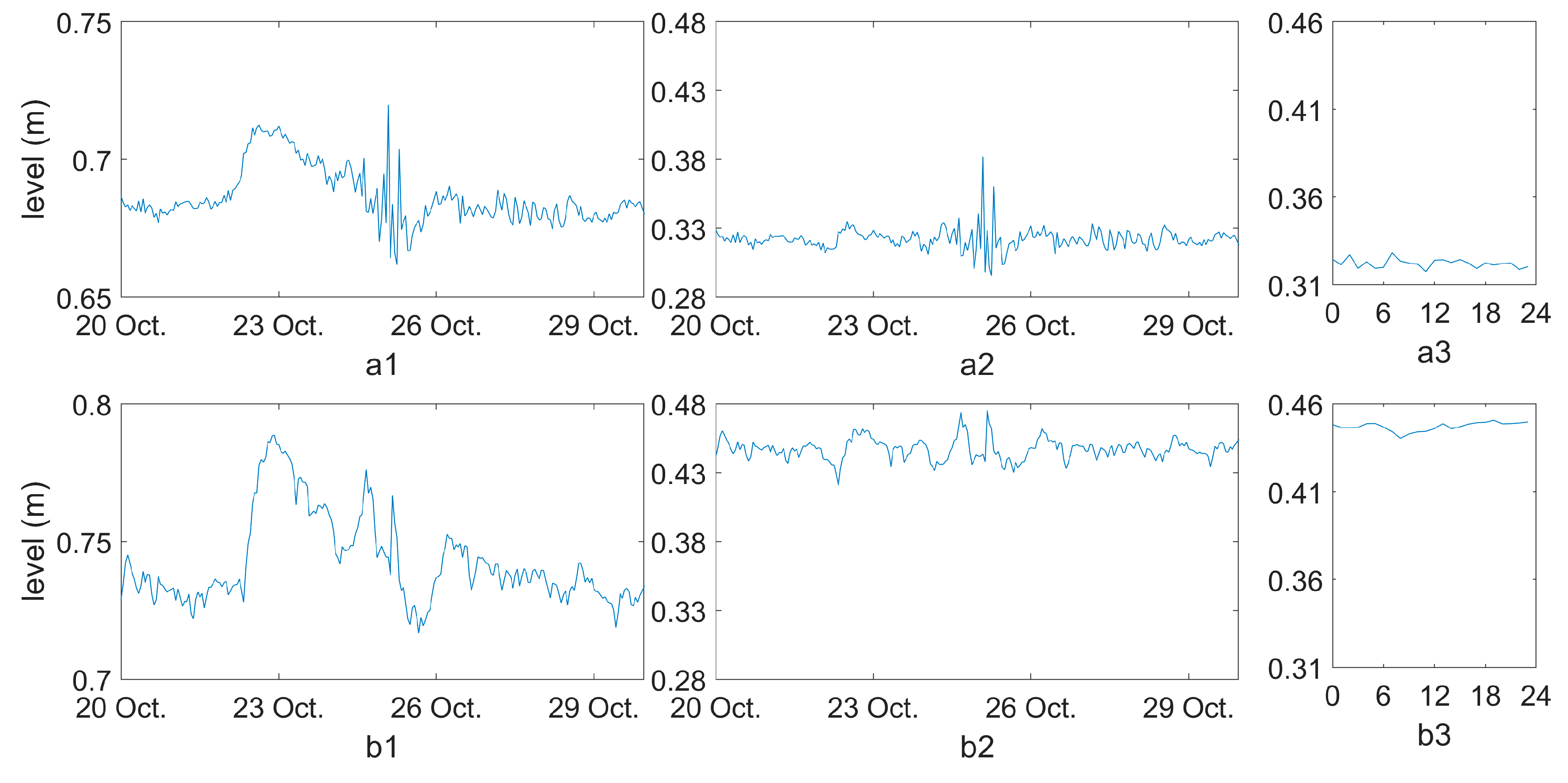
The average diurnal profile of streamwater level at both monitoring points had irregular fluctuations that do not satisfy the definition of a diurnal cycle. This was due mainly to rainfall events, which have strong responses in the change of the river water level. If the analysis window was restricted only to periods of baseflow, diurnal cycles could be observed for this parameter too (minima in the midday, maxima during late evening). The mean relative streamwater level was 0.786 m upstream of Suceava city and 0.895 m downstream. The standard deviation indicated a higher difference between the two points: 0.121 m upstream and 0.305 m downstream. The increased variability of the water level downstream of Suceava city is to be attributed mainly to water runoff from impervious urban areas because of tributaries that flow into the Suceava River between the two sampling points. These tributaries have small discharges at baseflow and receive some of the pluvial drainage from the metropolitan area (especially Șcheia, Cetății, Dragomirna, and Podu Vatafului creeks [9]).
2.4. Analysis Methods
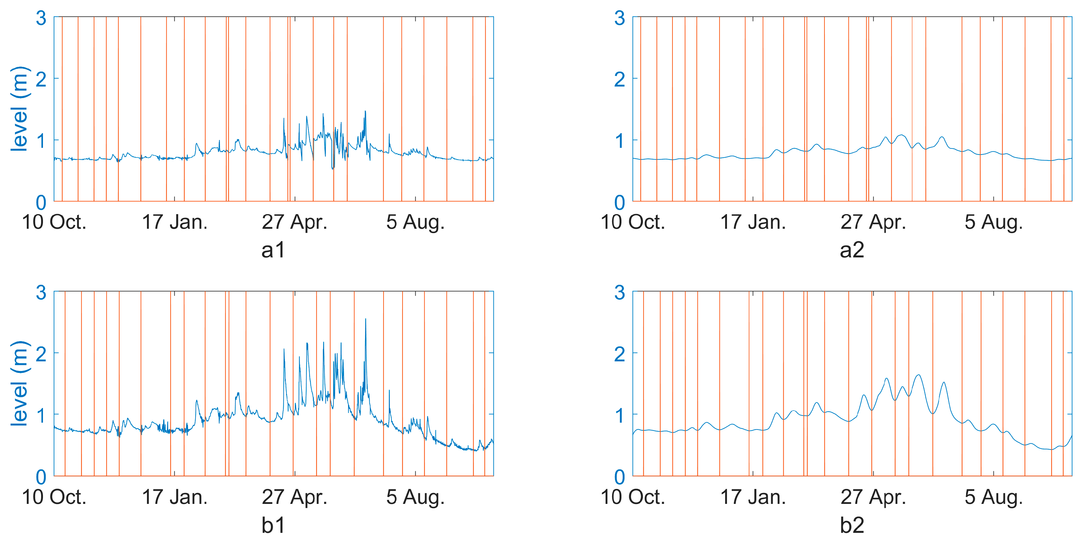
Variations in flow rates/water level can cause important changes in the diurnal profile of other streamwater parameters. Increases in water level have a clear cause, rainfall, and the slow decline in water level is to be naturally expected until the next rainfall. For this reason, we chose the water level parameter as the control factor when analyzing SC, DO, ORP, and pH. More precisely, we analyzed the water level time series in order to choose the position and length of the analysis windows used for comparing the diurnal profiles of the other parameters. Because the increase in water level is the active change, we decided to split the water level time series into subsets whose ends were given by the minimum values between high waters (Figure 5). A time interval between such minima would be a good case study to observe changes in diurnal cycles induced by peaks in flow rates.
Data analysis consisted of four major steps: (1) applying the multiresolution and wavelet analysis on raw level data in order to obtain time intervals for case studies; (2) smoothing the time series of water level, SC, DO, ORP, and pH, obtaining the evolution of diurnal cycles with the super-daily trends removed and normalizing the remnant time series for the upstream-downstream comparison; (3) computing the average diurnal profiles for case study time intervals from the normalized time series; and (4) comparing the case study time intervals from the normalized time series through the wavelet coherence analysis.
Prerequisites for the proposed analysis methodology were: MATLAB software (for all steps), the three script files found in the Supplementary Material of this paper (for the first three major steps), the cross wavelet and wavelet coherence toolbox of Aslak Grinsted [26] (https://www.mathworks.com/matlabcentral/fileexchange/47985-cross-wavelet-and-wavelet-coherence), data loaded/created in MATLAB workspace consisting of two variables named “upstream” and “downstream”, which were 1D column vectors representing one parameter per monitoring point and having a length equal to a multiple of 24 (because data in this study was sampled 24 times per day).
The first step had four stages:
- Applying the maximal overlap discrete wavelet transform to the water level data from both monitoring points. This was acquired with the function modwt, which has the following syntax:where x is the real-valued signal; wname is the name of an orthogonal wavelet, which, in our case, was ‘haar’; and n represents the desired number of levels of detail coefficients—7 in this case;y = modwt(x,wname,n),
- Executing the multiresolution analysis based on modwt, with the function modwtmra, which had a similar syntax:where wname should be the same as that used with modwt;z = modwtmra(y,wname),
- Extracting the approximation left from the raw data after the removal of the detail coefficients. This is a vector from the multiresolution analysis matrix and represents the simplified data shown in Figure 5;
- Identifying the local minima on the simplified data (marked with vertical red lines in Figure 5). Note that the positions of minima in the two monitoring points are rarely the same due to differences imposed by geographic location. When selecting the case study time intervals for steps 3 and 4, time intervals delineated by local minima from the two time series were superposed and only the common interval was then selected for being reduced to a size that was multiple of 24 (by starting and ending the case study time series at midnight).
The wavelet decomposition and the maximal overlap discrete wavelet transform were applied previously in a few studies concerning some streamwater parameters, such as water level, DO, and pH [3,5,27,28], which also offer the mathematical description of the mentioned wavelet analyses. Haar wavelet was successfully tested for water parameters [29].
The second step had 3 stages:
- Smoothing the raw time series by using the smooth function, which had the following syntax:where the method used here was the moving average (moving; lowpass filter with coefficients equal to the reciprocal of the span) and the span was equal to a day (24). Note that, due to software limitations, span was reduced by 1 to an even number;yy = smooth(x,span,method),
- Obtaining the detrended diurnal cycle from raw data after subtracting the smoothed data from it;
- Normalizing the detrended time series between 0 and 1 for the upstream-downstream comparison purposes.
Steps 1 and 2 were computed by executing the analyze command line in MATLAB console. This line applies the codes written in the analyze.m script file found in the Supplementary Material. After this command line was applied, two new variables, normalisedU and normalisedD, were created in the workspace and represented the normalized data from upstream and downstream, respectively, obtained at step 2, stage 3 (some other intermediary variables were also created in the workspace, but were handled automatically by codes). The analyze command line also generated a graphical output, similar to Figure 5, and was applied to water level data. In order to obtain only normalized data (as in step 2), for the other streamwater parameters, the command line transform had to be executed, which used the transform.m script file (in the Supplementary Material) and generated the variables PnormalisedU and PnormalisedD.
All of the new time series from (P)normalisedU and (P)normalisedD were involved in step 3, because they served as the source of data that was cut for case studies by using the time intervals established at the end of step 1. Data selected for case studies had to be included in two new variables, named CSnormalisedU and CSnormalisedD.
Step 3 had only one stage, when the average diurnal profile was computed, and some graphical outputs were generated, as in Figure 6 (using the newly generated variables CSprofileU and CSprofileD). This step was executed with the command line compare (with codes written in the compare.m script file, found in the Supplementary Material).
Step 4 had one stage and used the wtc function which performs the wavelet coherence analysis between two variables and has the syntax:
where a and b are values from the upstream and downstream parameters, respectively (e.g., normalisedU, PnormalisedU, or CSnormalisedU). The analysis produced scalograms that indicated how strong two signals co-vary by using a power spectrum and phase arrows. Also, periodicities in signals were tested against the AR1 red noise through a Monte Carlo test and the relevant results were marked with a black line. The wavelet coherence used the Morlet mother wavelet because it is best suited for comparing time series with non-linear processes [26,30]. Wavelet coherence mechanics and results were described by previous studies that applied this type of analysis to hydrological time series [26,31]. The script files used in this methodology are included in the Supplementary Material and described in an accessible manner between the lines of codes contained in the files.
wtc(a,b),
3. Results and Discussion
The analysis of the major convolutions/waves of water level during a year led us to select two subsets of time series that should serve as relevant case studies of changes in diurnal profiles depending on water level variability. Case study 1 comprised 23 days during a period of intense rainfalls and high waters (17 June–9 July 2019; Figure 6, Figure 7, Figure 8, Figure 9 and Figure 10), while case study 2 comprised 10 days during the autumn baseflow (20–29 October 2018; Figure 11, Figure 12, Figure 13, Figure 14 and Figure 15). The length of the subsets with common major evolutions could be increased or decreased depending on the number of levels of detail coefficients of the maximal overlap discrete wavelet transform, which in our case was set to 7.
Depending on the characteristics of water flow or the need for longer/shorter subsets, the number of levels of detail coefficients could be edited in the anlyze.m script file. The smaller the number of levels, the fewer details that were removed from the original time series through decomposition. The subsets were very numerous and small; more levels removed more details and generated and abstracted the approximation of the original data, where only a few subsets could be assessed. Therefore, the choice of decomposition level depends on the user/author [32], as it is the choice of applying the multiresolution analysis only on the water level or on other parameter/all parameters. Available orthogonal wavelets in MATLAB that can replace the Haar wavelet (‘haar’) option are: Daubechies (‘dbN’), Symlets (‘sym4‘ or ‘symN’), Coiflets (‘coifN’), and Fejér–Korovkin (‘fkN’).
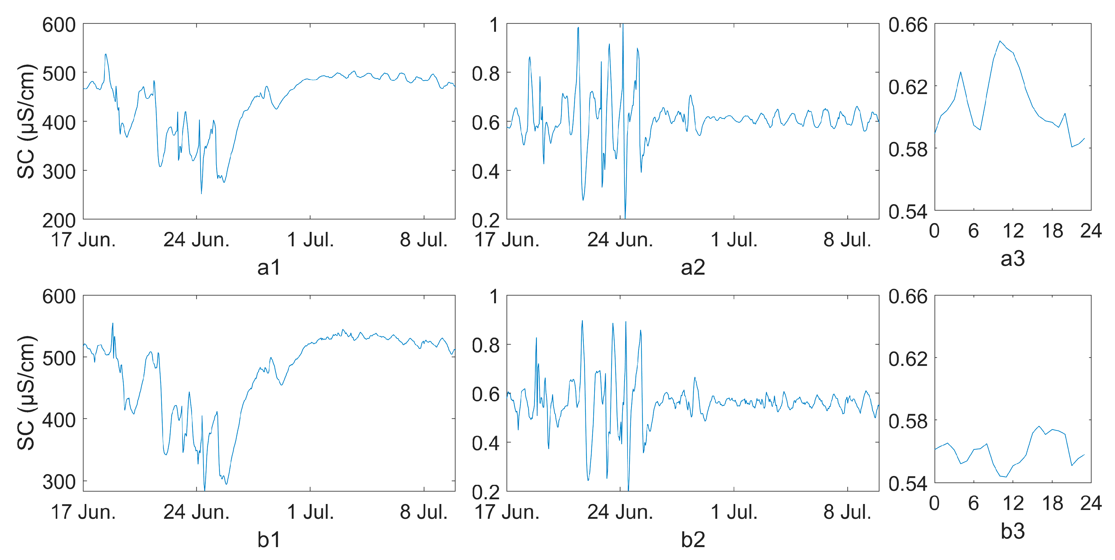
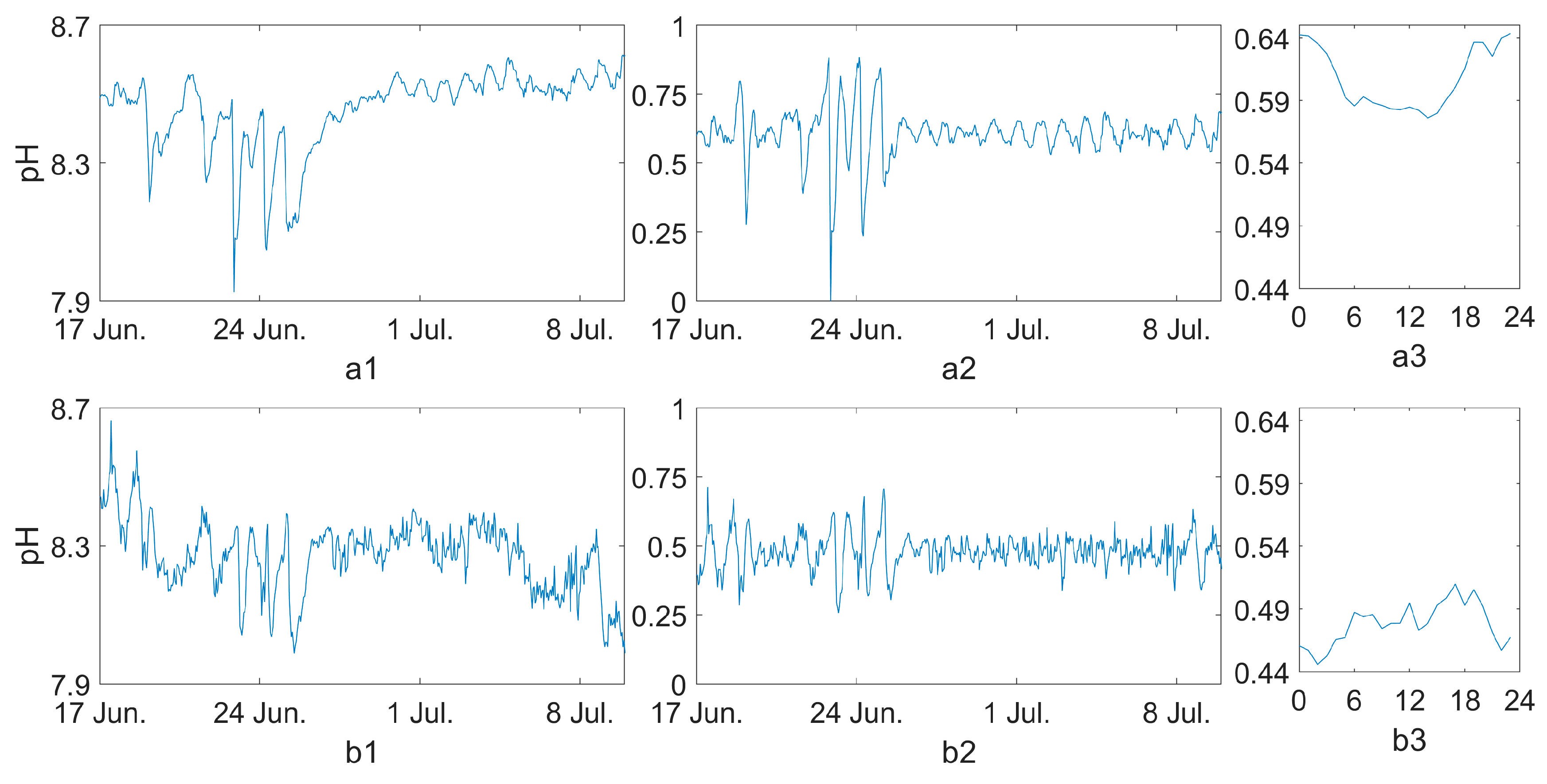
Distinct average diurnal profiles can be observed for any water parameter in case study 1, except for SC (Figure 7), which was very sensitive to water level oscillations during high waters. Such time intervals explain the complex shape of the average diurnal profile of SC calculated for a year (Figure 4a1). Another parameter that had the diurnal cycle easily altered by important changes in water level was pH (Figure 10). Changes in the shapes and positions of the diurnal cycles occurred in the average diurnal profile of DO (Figure 8); at both monitoring points, diurnal maxima moved towards midday or late morning (Figure 4b).
The script files analyze.m and transform.m allowed for editing the smoothing and detrending methods. The smoothing can be done with a filter other than the default moving average. Available filters were: ‘lowess’, a local regression with weighted linear least squares and a 1st degree polynomial model; ‘loess’, the same as the previous, but with a 2nd degree polynomial model; ‘rlowess’ or ‘rloess’, robust versions of ‘lowess’ or ‘loess’ with lower weight for outliers in the regression; ‘sgolay’, a Savitzky–Golay filter. Also, smoothing could be set to be more or less aggressive with the increase or decrease in the span number.
The detrending technique may be different than the proposed difference between the raw and smoothed date. A method with a similar ability to remove general and seasonal trends might show the difference between adjacent elements, if the following syntax is used: y=diff(x).
We inserted a few codes between the lines that execute smoothing and detrending. These are aimed at helping those that intend to obtain detrended values that can no longer be normalized. Instead, a detrended time series with absolute values, similar to those of the raw time series (but lower), will be obtained. It is necessary that this option is applied only to data with inter-diurnal variations significantly higher than the annual oscillation and with weak variability in the diurnal cycle (dedicated variables created in the workspace were differenceX and subtrendX, where X is U (upstream data) or D (downstream data)).
The time interval of case study 2 belonged to the autumn baseflow, where the main aperiodic changes were caused by a few rainfalls. For the first time, SC average diurnal profiles at both monitoring points were similar (Figure 12). This led to the conclusion that, during periods of baseflow, which are longer than the periods affected by intense rainfalls, this similarity is frequent and only these average diurnal profiles might be considered relevant for describing various persistent riverine processes.
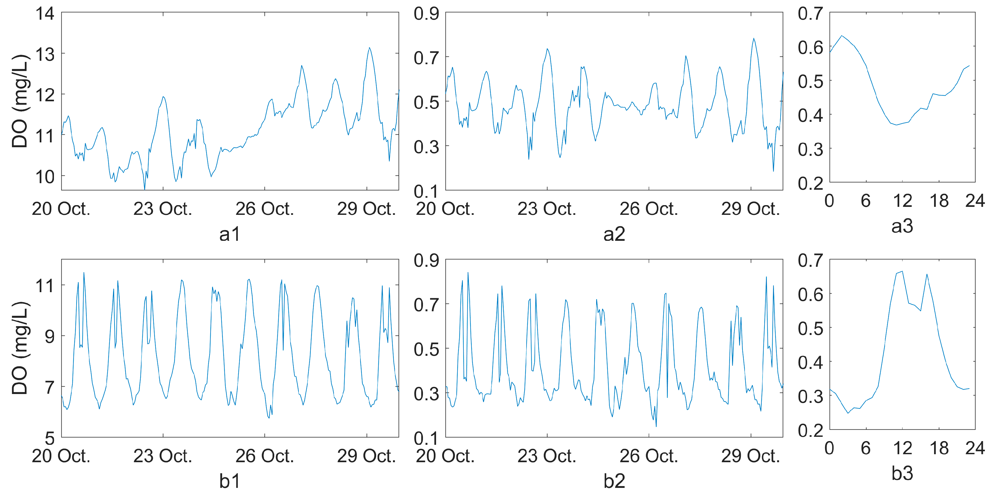
Another interesting observation was linked to the diurnal behavior of DO at the downstream monitoring point (Figure 13b). The diurnal cycle had the same relative position of minima as observed in the annual diurnal profile (Figure 4b2), but recorded maxima in two secondary peaks superposed on the diurnal oscillation. Various processes may co-generate this double-peaked shape, including the urban heat island (because the water is measured at the downstream point after passing through the middle of Suceava city). A change also occurred in the hourly position of the maximum value of the DO average diurnal profile: it occurred early in the morning, instead of late evening, as in the annual profile.
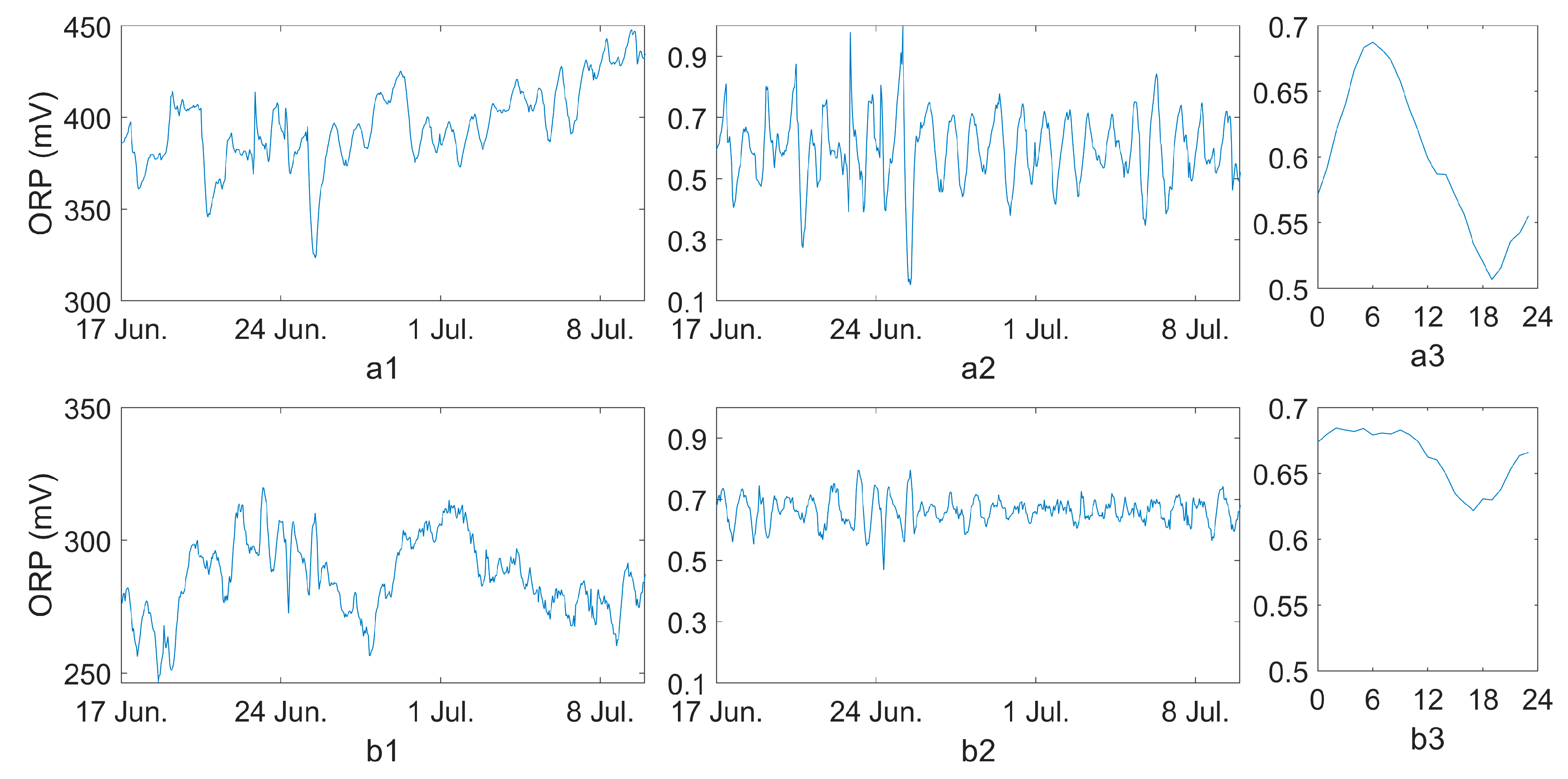
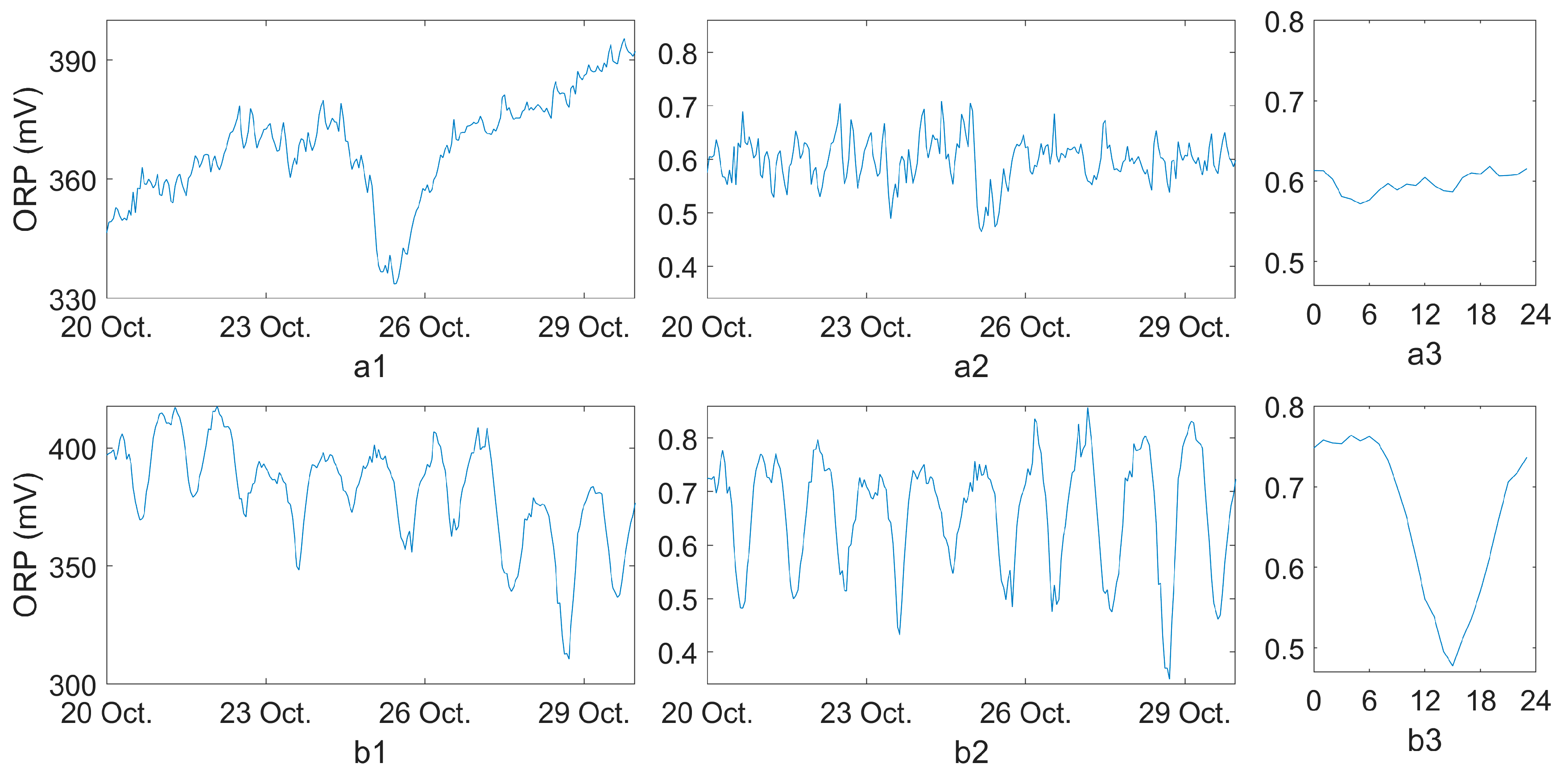
The diurnal oscillations of ORP and pH were strongly affected by rainfalls during baseflow at the upstream monitoring point. This was caused by the weak intensity of the diurnal cycle, which became easily modifiable by quasi-random events. In contrast, at Tișăuți, the diurnal cycles of ORP and pH had oscillations stronger than the general trend, which was different at the downstream point than at the upstream point. Given the fact, discussed previously, that the metropolitan area modifies the averages and standard deviations of the measured parameters, we may assume that the stronger diurnal cycle of ORP and pH at the downstream point is regulated by Suceava city. This may also explain why pH values were not lowered by rainfalls, which, by contrast, cause relatively sudden drops at the upstream point. This latter behavior is natural because of the acidic nature of the raindrops, which dissolve gases, such as CO2, from the atmosphere. The amplitude of the diurnal cycle of pH had amplitudes much greater than 0.2 units, which might induce stress to aquatic fauna. The high variability of pH combined with the low DO during some periods of the year could have caused fish mortality, as reported in June 2018 near the downstream monitoring point (at Lisaura). During the period investigated by us in 2018 and 2019, the minimum DO value was 5.2 mg/L upstream of Suceava city and 2.1 mg/L (critical value) downstream of the city. Pollutants from the wastewater treatment plant of Suceava city contributed to the observed values of the monitored parameters, especially when the plant has difficulties in treating the wastewaters according to specific regulations [10]. The changes in the metropolitan area toward higher imperviousness [10] and the changes in climate toward an increased average air temperature in the study area [33] will generate higher pH oscillations and lower DO concentrations downstream of Suceava city and more fish mortality events are to be expected in the near future.
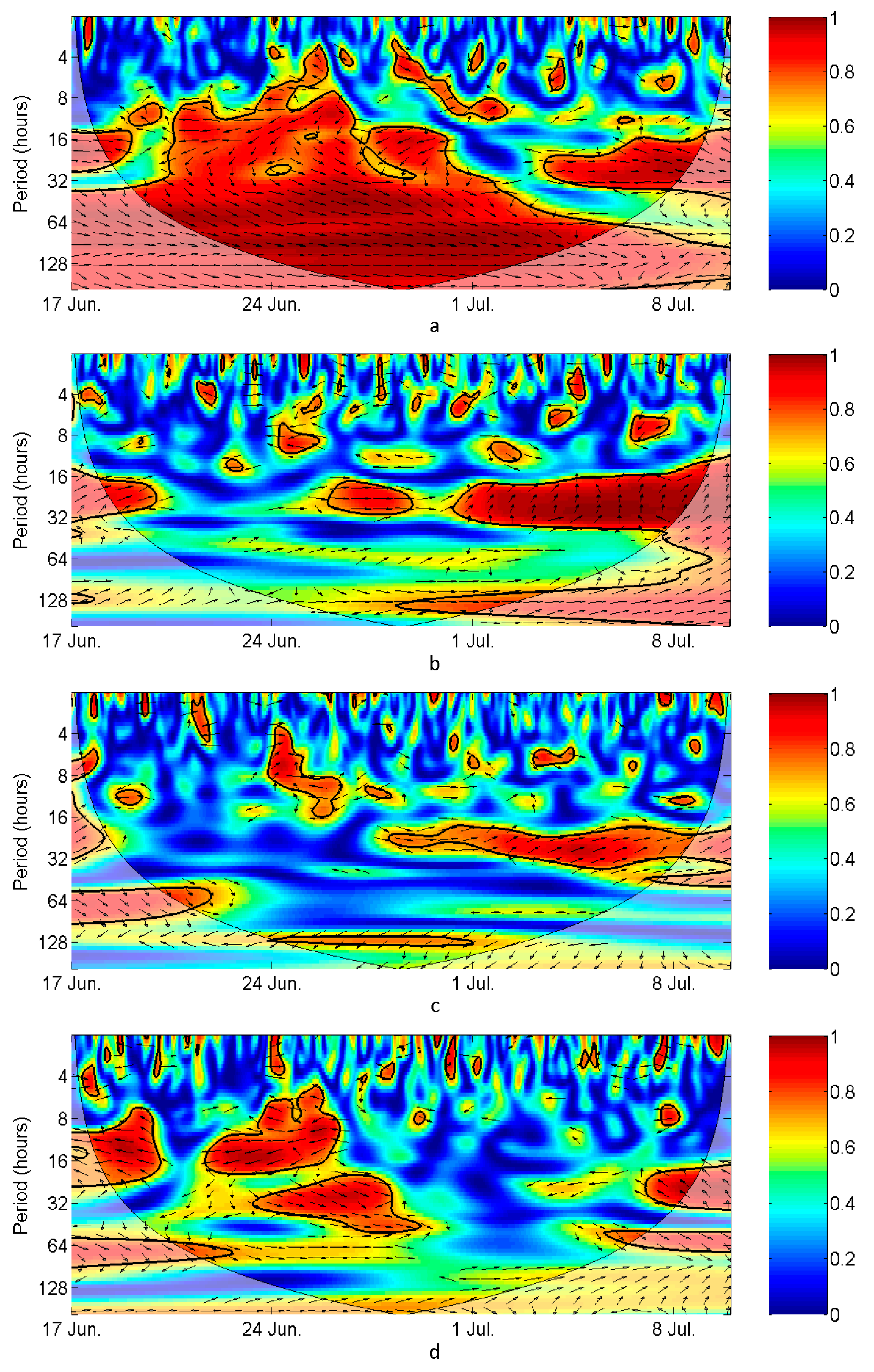
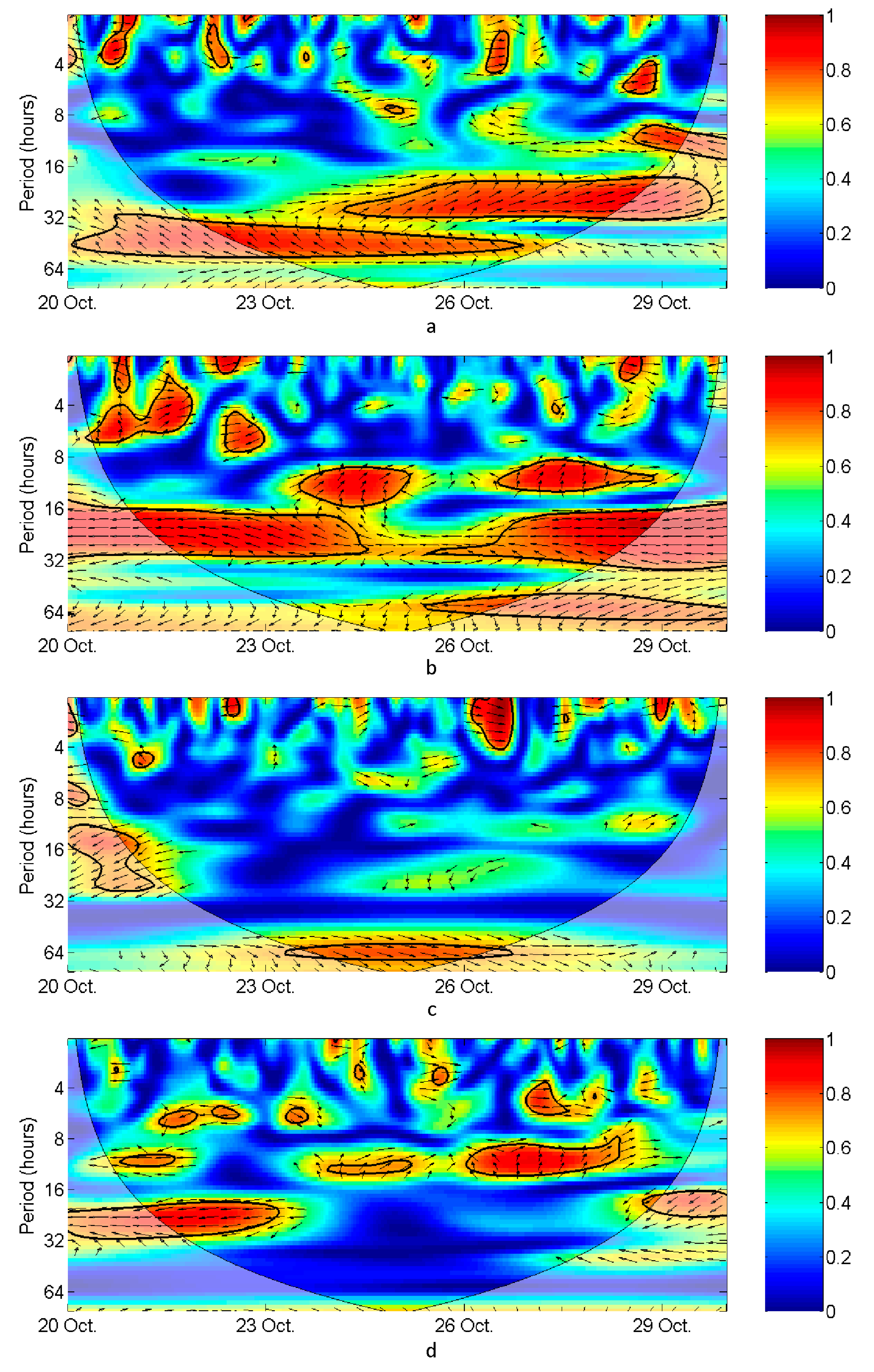
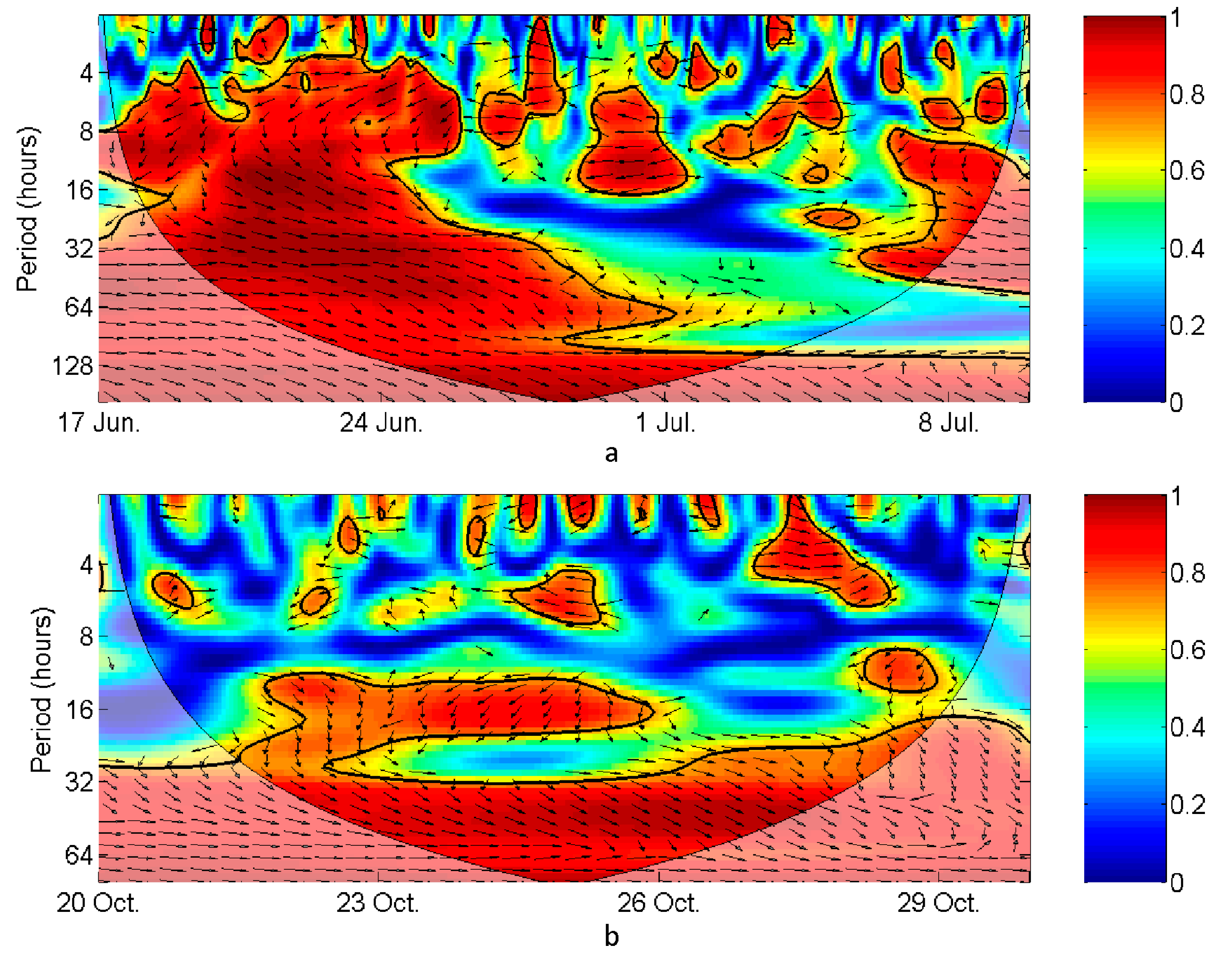
The wavelet coherence analysis allowed us to find time intervals when the diurnal cycle was statistically significant (0.95) at both monitoring points at the same time and to observe the temporal changes of the phasing of this cycle (Figure 16, Figure 17 and Figure 18; arrows pointing right indicate in-phase evolution and anti-phase when pointing left). At a first glance, we observed the high extension of the area with high power (red) on SC scalograms, very similar to that of the water level scalograms. Except for the diurnal band observed for SC in October 2018 (Figure 17a), the high power indicates only very good co-variance over periods greater than 32/64 h; the weak coherence at high frequencies is caused by the disturbing effect of high waters.
The only persistent coherence between time series recorded upstream and downstream in both case studies was observed for DO (Figure 16b and Figure 17b). During June–July 2019, the diurnal cycles at both monitoring points were in phase or almost in phase, while during October 2018 they were in obvious anti-phase on both sides of the cone of influence (which separates time intervals affected by the edge effects from those that are not affected). Moments when other parameters had coherent evolution of the diurnal cycles in both monitoring points were at the end of June and beginning of July 2019 for ORP and in October 2018 for pH.
4. Conclusions
This study is the first one to use high-frequency (hourly) measurements done over a 365-day interval in the analysis of the temporal and spatial evolution of SC, DO, ORP, and pH of the Suceava River. Raw and normalized time series from case studies, together with average diurnal profiles and scalograms of the wavelet coherence analysis, indicate distinct diurnal evolutions of the selected parameters over time, which cannot be deduced from the annual average diurnal profiles. Important differences in the shape and hourly position of the diurnal cycles of the same parameter occurred between the upstream and downstream monitoring points, despite of the short distance that separated them. Important changes in the monitored water parameters are caused by Suceava city, located between the selected monitoring points.
The case studies time intervals were selected objectively by using the multiresolution analysis of the maximal overlap discrete wavelet transform applied to water level data. The removal of detail coefficients from the raw water level data allowed for detecting the major variations that impose changes in other water parameters. These major variations were generated by increases in water levels due to rainfalls. The time series of SC, DO, ORP, and pH were detrended prior to comparing their average diurnal profiles at the upstream and downstream monitoring points for a better understanding of the diurnal cycles.
The pair of monitoring points, located upstream and downstream of Suceava city, allowed for measuring the impact of urban wastewaters on the Suceava River. The specific conductivity was higher downstream of the city (yearly averages: 483.1 µS/cm upstream, 549 µS/cm downstream) because of both treated and untreated waters discharged directly or indirectly into the Suceava River. Dissolved oxygen mean annual values were 10.6 mg/L (upstream) and 8.82 mg/L (downstream). The low downstream values are caused by pollutants in water, which consume oxygen in chemical reactions, and because of the urban heat island, which led to warmer waters, less able to dissolve oxygen from the atmosphere.
Three MATLAB script files are provided for a fast comparison process, especially useful when using big data. Codes within the script files are explained and possible variations of the analyses are proposed for a more flexible approach when different data are analyzed. Options include, but are not limited to, variations of the wavelet type, decomposition level, and detrending methods. The proposed methodology is best suited for comparing results from case studies.
Supplementary Materials
The following are available online at https://www.mdpi.com/2073-4441/11/12/2524/s1. Supplementary Material (a zip archive containing three MATLAB .m script files).
Author Contributions
Conceptualization, A.-E.B. and A.G.; Data curation, A.-E.B. and C.F.; Investigation, A.-E.B. and D.I.O.; Methodology, A.-E.B. and C.F.; Resources, A.-E. B., A.G., and D.I.O.; Supervision, A.G.; Visualization, D.I.O. and C.F.; Writing—original draft, A.-E.B.; Writing—review & editing, A.G.
Funding
This research was funded by CNCS - UEFISCDI, project number PN-III-P1-1.1PD-2016-2106.
Acknowledgments
Wavelet coherence software was provided by A. Grinsted. This study was supported by data obtained within the research project SQRTDA (Streamwater Quality Real-Time Data Analysis). This work was supported by a grant of Ministry of Research and Innovation, CNCS - UEFISCDI, project number PN-III-P1-1.1PD-2016-2106, within PNCDI III.
Conflicts of Interest
The authors declare no conflict of interest. The funders had no role in the design of the study; in the collection, analyses, or interpretation of data; in the writing of the manuscript, or in the decision to publish the results.
References
- Labat, D. Recent advances in wavelet analyses: Part 1. A review of concepts. J. Hydrol. 2005, 314, 275–288. [Google Scholar] [CrossRef]
- Labat, D.; Ronchail, J.; Guyot, J.L. Recent advances in wavelet analyses: Part 2—Amazon, Parana, Orinoco and Congo discharges time scale variability. J. Hydrol. 2005, 314, 289–311. [Google Scholar] [CrossRef]
- Lee, M.; You, Y.; Kim, S.; Kim, K.T.; Kim, H.S. Decomposition of Water Level Time Series of a Tidal River into Tide, Wave and Rainfall-Runoff Components. Water 2018, 10, 1568. [Google Scholar] [CrossRef]
- Evrendilek, F.; Karakaya, N. Monitoring diel dissolved oxygen dynamics through integrating wavelet denoising and temporal neural networks. Environ. Monit. Assess. 2014, 186, 1583. [Google Scholar] [CrossRef] [PubMed]
- Parmar, K.S.; Bhardwaj, R. Wavelet and statistical analysis of river water quality parameters. Appl. Math. Comput. 2013, 219, 10172–10182. [Google Scholar] [CrossRef]
- Baker, M.E.; Schley, M.L.; Sexton, J.O. Impacts of Expanding Impervious Surface on Specific Conductance in Urbanizing Streams. Water Resour. Res. 2019, 55, 6482–6498. [Google Scholar] [CrossRef]
- Rajwa-Kuligiewicz, A.; Bialik, R.J.; Rowiński, P.M. Wavelet Characteristics of Hydrological and Dissolved Oxygen Time Series in a Lowland River. Acta Geophys. 2016, 64, 649–669. [Google Scholar] [CrossRef]
- Somers, K.A.; Bernhardt, E.S.; Grace, J.B.; Hassett, B.A.; Sudduth, E.B.; Wang, S.; Urban, D.L. Streams in the urban heat island: Spatial and temporal variability in temperature. Freshw. Sci. 2013, 32, 309–326. [Google Scholar] [CrossRef]
- Kinouchi, T.; Yagi, H.; Miyamoto, M. Increase in stream temperature related to anthropogenic heat input from urban wastewater. J. Hydrol. 2007, 335, 78–88. [Google Scholar] [CrossRef]
- Briciu, A.-E. Studiu de Hidrologie Urbană în Arealul Municipiului Suceava (Urban Hydrology Study in Suceava Municipality Area); Ştefan cel Mare University Publishing House: Suceava, Romania, 2017. [Google Scholar]
- Gribovszki, Z.; Szilágyi, J.; Kalicz, P. Diurnal fluctuations in shallow groundwater levels and streamflow rates and their inter-pretation—A review. J. Hydrol. 2010, 385, 371–383. [Google Scholar] [CrossRef]
- Bond, B.J.; Jones, J.A.; Moore, G.; Phillips, N.; Post, D.; McDonnell, J.J. The zone of vegetation influence on baseflow revealed by diel patterns of streamflow and vegetation water use in a headwater basin. Hydrol. Process. 2002, 16, 1671–1677. [Google Scholar] [CrossRef]
- Nimick, D.A.; Cleasby, T.E.; McCleskey, R.B. Seasonality of diel cycles of dissolved trace-metal concentrations in a Rocky Mountain stream. Environ. Geol. 2005, 47, 603–614. [Google Scholar] [CrossRef]
- Briciu, A.-E.; Oprea-Gancevici, D.I. Diurnal thermal profiles of selected rivers in Romania. SGEM2015 Conf. Proc. 2015, 1, 221–228. [Google Scholar]
- Briciu, A.-E.; Mihăilă, D.; Mihăilă, D. Short, medium and long term stochastic analysis of the Suceava River pollution evolution in the homonymous city. SGEM2012 Conf. Proc. 2012, 3, 809–816. [Google Scholar]
- Teodosiu, C.; Cojocariu, C.; Musteret, C.P.; Dăscălescu, I.G.; Caraene, I. Assessment of human and natural impacts over water quality in the Prut River basin, Romania. Environ. Eng. Manag. J. 2009, 8, 1439–1450. [Google Scholar] [CrossRef]
- Florescu, D.; Ionete, R.E.; Sandru, C.; Iordache, A.; Culea, M. The influence of pollution monitoring parameters in characterizing the surface water quality from Romania southern area. Rom. J. Phys. 2011, 56, 1001–1010. [Google Scholar]
- Batrînescu, G.; Bîrsan, E.; Vasile, G.; Stănescu, B.; Stănescu, E.; Păun, I.; Petrescu, M.; Filote, C. Identification of the aquatic ecosystems integrating variables in the Suceava hydrographic basin and their correlations. J. Environ. Prot. Ecol. 2011, 12, 1627–1643. [Google Scholar]
- Vasilache, V.; Filote, C.; Crețu, M.A.; Sandu, I.; Coisin, V.; Vasilache, T.; Maxim, C. Monitoring of groundwater quality in some vulnerable areas in Botoșani County for nitrates and nitrites based pollutants. Environ. Eng. Manag. J. 2012, 11, 471–479. [Google Scholar] [CrossRef]
- Marusic, G.; Sandu, I.; Vasilache, V.; Filote, C.; Sevcenco, N.; Crețu, M.-A. Modeling of spacio-temporal evolution of fluoride dispersion in “river-type” systems. Rev. Chim. 2015, 66, 503–506. [Google Scholar]
- Iticescu, C.; Georgescu, L.P.; Topa, C.M. Assessing the Danube water quality index in the city of Galați, Romania. Carpath. J. Earth Environ. Sci. 2013, 8, 155–164. [Google Scholar]
- Romanescu, G.; Crețu, M.A.; Sandu, I.G.; Păun, E.; Sandu, I. Chemism of streams within the Siret and Prut drainage basins: Water resources and management. Rev. Chim. 2013, 64, 1416–1421. [Google Scholar]
- Briciu, A.-E.; Toader, E.; Romanescu, G.; Sandu, I. Urban Streamwater Contamination and Self-purification in a Central-Eastern European City. Part I. Rev. Chim. 2016, 67, 1294–1300. [Google Scholar]
- Briciu, A.-E.; Toader, E.; Romanescu, G.; Sandu, I. Urban Streamwater Contamination and Self-purification in a Central-Eastern European City. Part B. Rev. Chim. 2016, 67, 1583–1586. [Google Scholar]
- Florescu, G.; Briciu, A.-E.; Hutchinson, S.M. An assessment of in-channel alluvia (aits) in the Suceava River near Suceava city, NE Romania. Georeview 2019, 29, 84–97. [Google Scholar]
- Grinsted, A.; Moore, J.C.; Jevrejeva, S. Application of the cross wavelet transform and wavelet coherence to geophysical time series. Nonlinear Process. Geophys. 2004, 11, 561–566. [Google Scholar] [CrossRef]
- Seo, Y.; Choi, Y.; Choi, J. River Stage Modeling by Combining Maximal Overlap Discrete Wavelet Transform, Support Vector Machines and Genetic Algorithm. Water 2017, 9, 525. [Google Scholar]
- Chen, Y.; Guan, Y.; Shao, G.; Zhang, D. Investigating Trends in Streamflow and Precipitation in Huangfuchuan Basin with Wavelet Analysis and the Mann-Kendall Test. Water 2016, 8, 77. [Google Scholar] [CrossRef]
- Parmar, K.S.; Bhardwaj, R. Analysis of Water Parameters Using Haar Wavelet (Level 3). Int. J. Curr. Eng. Technol. 2012, 2, 166–171. [Google Scholar]
- Torrence, C.; Compo, G.P. A practical guide to wavelet analysis. Bull. Am. Meteorol. Soc. 1998, 79, 61–78. [Google Scholar] [CrossRef]
- Briciu, A.-E. Wavelet analysis of lunar semidiurnal tidal influence on selected inland rivers across the globe. Sci. Rep. 2014, 4, 4193. [Google Scholar] [CrossRef]
- Yang, M.; Sang, Y.-F.; Liu, C.; Wang, Z. Discussion on the Choice of Decomposition Level for Wavelet Based Hydrological Time Series Modeling. Water 2016, 8, 197. [Google Scholar] [CrossRef]
- Mihăilă, D.; Briciu, A.-E. Actual climate evolution in the NE Romania. Manifestations and consequences. SGEM2012 Conf. Proc. 2012, 4, 241–252. [Google Scholar]
- Hatvani, I.G.; Clement, A.; Korponai, J.; Kern, Z.; Kovács, J. Periodic signals of climatic variables and water quality in a river—Eutrophic pond—Wetland cascade ecosystem tracked by wavelet coherence analysis. Ecol. Indic. 2017, 83, 21–31. [Google Scholar] [CrossRef] [Green Version]
Figure 1.
Map of the study area, including the location of the monitoring points and the urban wastewater treatment plant (WTP).
Figure 1.
Map of the study area, including the location of the monitoring points and the urban wastewater treatment plant (WTP).

Figure 2.
Variations in the studied parameters of the Suceava River at the upstream monitoring point (Mihoveni) from 10 October 2018 to 9 October 2019: (a) specific conductivity (SC), (b) dissolved oxygen (DO), (c) oxidation reduction potential (ORP), and (d) pH.
Figure 2.
Variations in the studied parameters of the Suceava River at the upstream monitoring point (Mihoveni) from 10 October 2018 to 9 October 2019: (a) specific conductivity (SC), (b) dissolved oxygen (DO), (c) oxidation reduction potential (ORP), and (d) pH.

Figure 3.
Variations in the studied parameters of the Suceava River at the downstream monitoring point (Mihoveni) from 10 October 2018 to 9 October 2019: (a) specific conductivity (SC), (b) dissolved oxygen (DO), (c) oxidation reduction potential (ORP), and (d) pH.
Figure 3.
Variations in the studied parameters of the Suceava River at the downstream monitoring point (Mihoveni) from 10 October 2018 to 9 October 2019: (a) specific conductivity (SC), (b) dissolved oxygen (DO), (c) oxidation reduction potential (ORP), and (d) pH.

Figure 4.
Average diurnal profiles of the selected parameters at the upstream (1) and downstream (2) monitoring points (horizontal axes in hours): (a) specific conductivity, (b) dissolved oxygen, (c) oxidation reduction potential, and (d) pH (data from 10 October 2018 until 9 October 2019; with the exception of DO, which was calculated from 6 December 2018 until 9 October 2019 due to missing data).

Figure 5.
Suceava River water level at the (a) upstream and (b) downstream monitoring points plotted by using (1) raw data and (2) simplified data computed with the multiresolution analysis. Vertical red lines represent the limits of time intervals between relevant minima (10 October 2018 –9 October 2019).

Figure 6.
Suceava River water level at the (a) upstream and (b) downstream monitoring points plotted as (1) raw data, (2) detrended and normalized data, and (3) the average diurnal profile of the normalized data (17 June–9 July 2019).
Figure 6.
Suceava River water level at the (a) upstream and (b) downstream monitoring points plotted as (1) raw data, (2) detrended and normalized data, and (3) the average diurnal profile of the normalized data (17 June–9 July 2019).

Figure 7.
Suceava River SC at the (a) upstream and (b) downstream monitoring points plotted as (1) raw data, (2) detrended and normalized data, and (3) the average diurnal profile of the normalized data (17 June 17–9 July 2019).
Figure 7.
Suceava River SC at the (a) upstream and (b) downstream monitoring points plotted as (1) raw data, (2) detrended and normalized data, and (3) the average diurnal profile of the normalized data (17 June 17–9 July 2019).

Figure 8.
Suceava River DO at the (a) upstream and (b) downstream monitoring points plotted as (1) raw data, (2) detrended and normalized data, and (3) the average diurnal profile of the normalized data (17 June 17–9 July 2019).
Figure 8.
Suceava River DO at the (a) upstream and (b) downstream monitoring points plotted as (1) raw data, (2) detrended and normalized data, and (3) the average diurnal profile of the normalized data (17 June 17–9 July 2019).

Figure 9.
Suceava River ORP at the (a) upstream and (b) downstream monitoring points plotted as (1) raw data, (2) detrended and normalized data, and (3) the average diurnal profile of the normalized data (17 June 17–9 July 2019).
Figure 9.
Suceava River ORP at the (a) upstream and (b) downstream monitoring points plotted as (1) raw data, (2) detrended and normalized data, and (3) the average diurnal profile of the normalized data (17 June 17–9 July 2019).

Figure 10.
Suceava River pH at the (a) upstream and (b) downstream monitoring points plotted as (1) raw data, (2) detrended and normalized data, and (3) the average diurnal profile of the normalized data (17 June 17–9 July 2019).
Figure 10.
Suceava River pH at the (a) upstream and (b) downstream monitoring points plotted as (1) raw data, (2) detrended and normalized data, and (3) the average diurnal profile of the normalized data (17 June 17–9 July 2019).

Figure 11.
Suceava River water level at the (a) upstream and (b) downstream monitoring points plotted as (1) raw data, (2) detrended and normalized data, and (3) the average diurnal profile of the normalized data (20–29 October 2018).
Figure 11.
Suceava River water level at the (a) upstream and (b) downstream monitoring points plotted as (1) raw data, (2) detrended and normalized data, and (3) the average diurnal profile of the normalized data (20–29 October 2018).

Figure 12.
Suceava River SC at the (a) upstream and (b) downstream monitoring points plotted as (1) raw data, (2) detrended and normalized data, and (3) the average diurnal profile of the normalized data (20–29 October 2018)..
Figure 12.
Suceava River SC at the (a) upstream and (b) downstream monitoring points plotted as (1) raw data, (2) detrended and normalized data, and (3) the average diurnal profile of the normalized data (20–29 October 2018)..

Figure 13.
Suceava River DO at the (a) upstream and (b) downstream monitoring points plotted as (1) raw data, (2) detrended and normalized data, and (3) the average diurnal profile of the normalized data (20–29 October 2018).
Figure 13.
Suceava River DO at the (a) upstream and (b) downstream monitoring points plotted as (1) raw data, (2) detrended and normalized data, and (3) the average diurnal profile of the normalized data (20–29 October 2018).

Figure 14.
Suceava River ORP at the (a) upstream and (b) downstream monitoring points plotted as (1) raw data, (2) detrended and normalized data, and (3) the average diurnal profile of the normalized data (20–29 October 2018).
Figure 14.
Suceava River ORP at the (a) upstream and (b) downstream monitoring points plotted as (1) raw data, (2) detrended and normalized data, and (3) the average diurnal profile of the normalized data (20–29 October 2018).

Figure 15.
Suceava River pH at the (a) upstream and (b) downstream monitoring points plotted as (1) raw data, (2) detrended and normalized data, and (3) the average diurnal profile of the normalized data (20–29 October 2018).
Figure 15.
Suceava River pH at the (a) upstream and (b) downstream monitoring points plotted as (1) raw data, (2) detrended and normalized data, and (3) the average diurnal profile of the normalized data (20–29 October 2018).

Figure 16.
Scalograms of the wavelet coherence analysis of some water parameters measured upstream and downstream during 17 June–9 July 2019: (a) SC, (b) DO, (c) ORP, and (d) pH.
Figure 16.
Scalograms of the wavelet coherence analysis of some water parameters measured upstream and downstream during 17 June–9 July 2019: (a) SC, (b) DO, (c) ORP, and (d) pH.

Figure 17.
Scalograms of the wavelet coherence analysis of some water parameters measured upstream and downstream during 20–29 October 2018: (a) SC, (b) DO, (c) ORP, and (d) pH.
Figure 17.
Scalograms of the wavelet coherence analysis of some water parameters measured upstream and downstream during 20–29 October 2018: (a) SC, (b) DO, (c) ORP, and (d) pH.

Figure 18.
Scalograms of the wavelet coherence analysis of the upstream and downstream water level during: (a) 17 June 17–9 July 2019 and (b) 20–29 October 2018.
Figure 18.
Scalograms of the wavelet coherence analysis of the upstream and downstream water level during: (a) 17 June 17–9 July 2019 and (b) 20–29 October 2018.

© 2019 by the authors. Licensee MDPI, Basel, Switzerland. This article is an open access article distributed under the terms and conditions of the Creative Commons Attribution (CC BY) license (http://creativecommons.org/licenses/by/4.0/).
Share and Cite
MDPI and ACS Style
Briciu, A.-E.; Graur, A.; Oprea, D.I.; Filote, C. A Methodology for the Fast Comparison of Streamwater Diurnal Cycles at Two Monitoring Points. Water 2019, 11, 2524. https://doi.org/10.3390/w11122524
AMA Style
Briciu A-E, Graur A, Oprea DI, Filote C. A Methodology for the Fast Comparison of Streamwater Diurnal Cycles at Two Monitoring Points. Water. 2019; 11(12):2524. https://doi.org/10.3390/w11122524
Chicago/Turabian StyleBriciu, Andrei-Emil, Adrian Graur, Dinu Iulian Oprea, and Constantin Filote. 2019. "A Methodology for the Fast Comparison of Streamwater Diurnal Cycles at Two Monitoring Points" Water 11, no. 12: 2524. https://doi.org/10.3390/w11122524
Note that from the first issue of 2016, this journal uses article numbers instead of page numbers. See further details here.