Reliability Assessment Model of Water Distribution Networks against Fire Following Earthquake (FFE)

1
School of Environment, Harbin Institute of Technology, Harbin 150090, China
2
Central and Southern China Municipal Engineering Design &Research Institute Co., Ltd., Wuhan 230031, China
3
Shenzhen ANSO Measurement &Control Instruments Co., Ltd., Shenzhen 518108, China
*
Author to whom correspondence should be addressed.
Water 2019, 11(12), 2536; https://doi.org/10.3390/w11122536
Submission received: 15 October 2019
/
Revised: 18 November 2019
/
Accepted: 27 November 2019
/
Published: 30 November 2019
(This article belongs to the Special Issue Resilient and Robust Water Distribution Systems: State-of-the-Art and Research Challenges)
Abstract
:Fire following earthquake (FFE) is a common secondary disaster that can inflict great damage to humans. A large number of seismic resilience evaluation methods have been proposed, but few of them consider the influence of FFE. In this study, a multi-scenario simulation based model was developed to evaluate the post-disaster performance of water distribution networks (WDNs) in supplying both firefighting flow and original demand under the effect of seismic damage and FFEs. Hypothetical earthquakes were generated and the spatial–temporal distribution of FFEs was simulated by the Poisson distribution model and the Weibull distribution model. The post-disaster performance was evaluated by two types of seismic reliability metrics. The developed model was applied to a WDN currently operating in China with eight pre-determined earthquake scenarios. The results showed that the firefighting flow was concentrated in the first few hours after the earthquake. Thus, the serviceability of both original demand and firefighting flow was influenced significantly within the first few hours, while little impact was observed after the concentrated firefighting flow was delivered. The proposed model quantified the WDN’s performance under specific seismic damage and potential FFEs, and can be used for the planning, design, and maintenance of WDNs.
1. Introduction
As a part of urban lifeline system, water distribution networks (WDNs) play an important role in satisfying the basic demands of residents, industrial production, firefighting, etc. To ensure safe water supply, reliability against hazards is a crucial consideration during the design and management of WDNs [1]. Although most components of WDNs are buried underground, they can still be threatened by various hazards such as power outrage, drastic temperature change, and pollution events [2]. Earthquake is one of the most severe hazards among them. Earthquakes can release enormous energy and create disruptive seismic waves which usually cause great damage to water systems. For example, over 1500 pipeline failures were caused by the Northridge earthquake in the Los Angeles area (1994, United States) [3], and the Kobe earthquake (1995, Japan) [4] caused more than 1600 failures. Despite the low frequency of earthquakes, once they occur they can cause long-term and large-scale damage to the functionality of WDNs.
In addition, earthquakes not only inflict great damage to WDNs itself, but cause simultaneous and catastrophic fires which can result in widespread economic damage and loss of life. Fire following earthquake (FFE), as an indirect seismic hazard, may cause more damage than the earthquake itself. For example, 138 fires following the Hanshin earthquake (1995, Japan) destroyed 7377 homes and killed more than 500 people [5]. The 1906 San Francisco earthquake and ensuing fire destroyed 492 city blocks and life loss was estimated at more than 3000 individuals [6]. The Great Kanto earthquake (1923, Japan) led to the most destructive post-earthquake fires in history with over 220,000 buildings burned, and in Tokyo city, 65,000 of 1,400,000 evacuees were killed by fire [7]. With the development of urbanization, it is predicted that the losses from FFEs exhibit a rising tendency and that the causes of FFEs will become more complex. Therefore, a model to assess the reliability of WDNs against FFEs is urgently needed.
The WDN’s seismic reliability design has always been a compromise between economic and safety issues [5]. In developing countries like China, firefighting cisterns are available only for important buildings due to their high construction and maintenance costs. According to National Code for Design on Building Fire Protection and Prevention in China (GB50016-2014), a firefighting cistern is only required for large warehouses or buildings higher than 50 m. For buildings taller than 28 m and shorter than 50 m, firefighting water is provided by connecting fire hydrants to WDNs and siamese connections on fire trucks. For lower buildings, fire trucks are required to provide fighting flow for first 10 minutes due to their limited volume. The rest of the fire water is supplied from the WDN by fire trucks. As stable and continuous fire water sources, WDNs and fire hydrants play an inevitable role in developing countries.
Meanwhile, if the WDN is seriously damaged by severe earthquake, it cannot be completely replaced by fire trucks or fire water cisterns. This is because conflagration is more likely to occur under severe earthquakes which generally require large amounts of water which cannot be completely provided by fire trucks and firefighting cisterns [3,4,5]. It was reported that a considerable part of fire protection work was greatly delayed because the underground storage of water was drained or the arrival of fire trucks was delayed after the Kobe earthquake (1995, Japan) [4]. Moreover, it was estimated that approximately 32–45 people could have been saved if the WDN had worked more quickly [4]. Thus, it could be concluded that although fire trucks and emergency water play an important role, reliable WDNs are still the main water source for fire fighting after earthquakes.
In this century, researchers have introduced a large amount of tools and metrics to help planners and engineers to evaluate WDN reliability with respect to potential disasters. The tools available in literature can be grouped in two main categories: attribute analysis-based and hydraulic model-based. Attribute analysis-based tools (e.g. graph theory [8,9]) do not require repeated sampling, so their results can be easily obtained. However, the results are calculated based on assumptions that might not fit to the problem in practice sometimes. In order to obtain more practical results, many studies are based on a hydraulic model [10,11,12,13,14]. In these studies, certain failure scenarios are generated and their results could characterize the WDN’s reliability and serviceability with a relatively low calculation speed.
The above studies on WDN’s were not aimed at specific kinds of hazards. In the past 30 years, reliability assessment models aiming at seismic hazards have been widely developed. HAZUS [15] was the first model to assess the economic losses of infrastructure caused by earthquakes. However, it is mainly used to assess earthquake damage rather than providing a detailed simulation of water system. Later, the American Lifelines Alliance (ALA) [16] proposed guidelines to evaluate the seismic damage on water systems, and many seismic reliability assessment studies followed these guidelines to create survival curves of pipes under seismic hazards [17]. Later studies began to propose a method for evaluating seismic reliability by hydraulic simulation using well-known hydraulic solvers and seismic simulations [18,19,20]. The latest and most popular assessment model is the graphical iterative response analysis for flow following earthquakes (GIRAFFE [21]), developed based on EPANET [22]. The graphical user interface of the model helps to visualize the results of the model, and it has been improved and validated through many case studies [23,24]. Yoo et al. [25] developed REVAS.NET to quantify the WDN’s hydraulic reliability with seismic reliability indicators by simulating probabilistic seismic events.
Although researchers have developed numerous models to quantify the functionality of WDNs under the effect of component failures caused by earthquake damage, few studies focused on the WDN functionality against secondary disasters, especially FFEs. Several attempts have been made to clarify the mechanism of ignition with probabilistic modeling [26,27,28,29]. HAZUS [15] used an empirical relationship in which the normalized average ignition frequency in urban areas is positively correlated with peak ground acceleration (PGA). These studies modeled the location and timetable of FFEs according to the urban geographic information, but due to the lack of hydraulic model, the influence of water supply system on fires was neglected.
This study aims to develop a model to systematically evaluate WDN reliability under the influence of seismic hazard and FFEs, with the goal of:
- (1)
- Evaluating the system’s functionality to supply adequate firefighting flows with a large number of components damaged by an earthquake. According to earthquake statistics in Japan [30], China [31], and the United States [15,32], most fire outbreaks occurred immediately after earthquake happened, leading to a large and concentrated demand of firefighting flow in a short time, which may be a heavy burden to the pipeline network.
- (2)
- Evaluating the system’s performance to satisfy original demand (e.g., residential demand, industrial demand, etc.) under the effect of both seismic damage and firefighting load.
In this study, probabilistic seismic damages and stochastic fire outbreaks are generated in specific areas, and the depth of earthquake failure is evaluated with seismic reliability indicators. The developed model was validated through a case study in MZ city, China and used for intensive research on how a water supply system hydraulically responds to seismic events.
2. Methodology
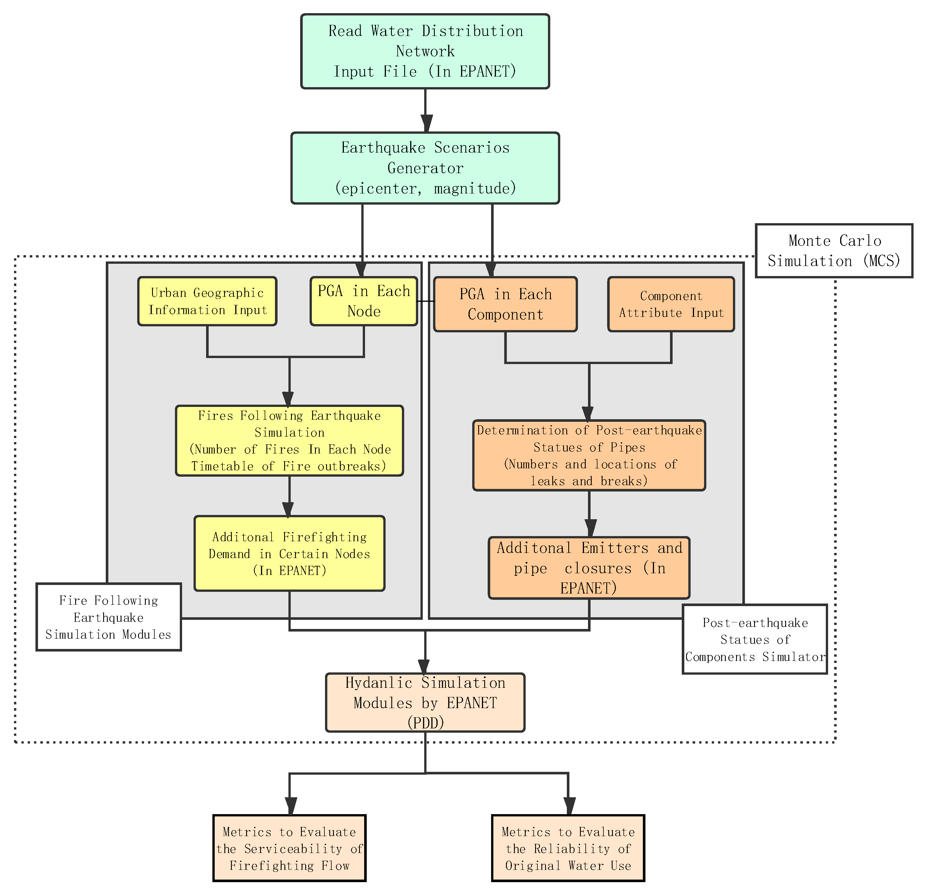
In this study, a model based on multi-scenario simulation was proposed. The model used a EPANET-MATLAB toolkit [33] to directly call EPANET functions [22] in the Matlab interface. Figure 1 shows the flowchart of the proposed model which consists of four modules: the earthquake scenario generator, fire following earthquake simulation modules, a component post-earthquake status simulator, and a hydraulic simulator. The earthquake scenario generator was developed to generate locations and magnitude of earthquakes, and then calculate peak ground acceleration (PGA) reached at each pipe and node (described in Section 2.1). For each generated earthquake scenario, Monte Carlo simulation (MCS) was used to estimate status of system components under seismic damage (Section 2.1) and the fire risks of each node (Section 2.2). To simulate the influence of FFEs and seismic damage in EPANET2, nodes with fire outbreaks were assigned additional firefighting demands and emitters were added to simulate pipe damage. For a higher accuracy of simulations, a pressure-dependent demand (PDD) model based on Abdy Sayyed’s research [28] was proposed (Section 2.3). Because the vast majority of fires occurred within three days after the earthquake, the simulation duration was set to 72 h. Then, reliability metrics were calculated according to the hydraulic simulation results (Section 2.4).
2.1. Earthquake Generation and Damage Determination
Firstly, the location of each epicenter and the earthquake magnitude is artificially designated to simulate an earthquake. Then, the seismic damage of each component was estimated by considering the attenuation of seismic wave, which was calculated according to the distance from epicenter and magnitude of earthquake. The seismic wave strength transmitted to the pipeline is quantified by peak ground acceleration (PGA). PGA is an index to quantify the movement of vibrations from the earthquake, which generally decrease with the distance from the epicenter increases. To estimate PGA in each node and pipe, a regression model by Pun and Amberaseys [34] was used:
where PGA is peak ground acceleration in g (gravity acceleration, 9.8 m/s2 in this study); M is earthquake magnitude; r is epicenter distance assuming a focal depth of 7.2 km; and r2 = R2 + 7.22, where R is the closest distance to the surface projection of a seismic source (km).
Log(PGA) = −0.789 + 0.2128M-log(r) + 0.00255r
To quantify the PGA in each component, network information such as the network layout, nodal coordinates, pipe diameters and lengths, and sizes of the pump and tanks should be read from the EPANET input file. After the PGA of each component is determined, the repair rate (RR, number of repairs/km pipes) is usually used to determine the status of a component. In this study, RR is estimated based on the equation developed by Isoyama et al. [35] and ALA [16].
where C1, C2, C3, and C4 represent the correction factors according to the pipe diameter, pipe material, topography, and liquefaction, respectively. A multiplier, 980, is added because in the equation by Isoyama et al. [35] the PGA is in cm/s, while in this research the PGA is in g.
RR = C1 × C2 × C3 × C4 × 0.00187 × PGA × 980
To determine the post-earthquake pipe status, ALA [16] recommended using Poisson distribution to quantify the number of breakages of one single pipe.
where x is a random variable denotes the number of events (i.e., pipe breaks), and is the average rate of repairs per unit length of pipe.
Thus the probability of break of an individual pipeline can be calculated by assuming k = 0 in Equation (3) and subtracting it from 1.
where is probability of pipe breakage and L indicates the pipe length.
Meanwhile, the probability of pipe leakage () is assumed to be five times higher than the probability of pipe breakage [16]. The failure of reservoirs and pumps are not calculated based on the work of Yoo et al. [25]. In this study, the post-earthquake component statuses can be classified as normal or has having leakage or breakage. Pipe leakage is defined as a small crack or hole on the pipe wall or at the joint with the main stream in pipes undamaged. Breakage means the pipe has been split into two pieces, which causes complete loss of transportation ability. This study used the same methods as Yoo et al. [1,25] and Choi et al. [36] to simulate leaks and breaks in EPANET2. A leaking pipe was modeled by adding an emitter in EPANET2 during hydraulic simulation. The pipe breakage was modeled by adding two emitters in both upstream and downstream and setting the broken pipe as closed in EPANET2. The leakage flow-pressure relationship was modeled according to the emitter discharge model adopted by EPANET2:
where is the discharge coefficient ( = ); is the discharge exponent ( in this study); A is the opening area of the leaking pipe in m2; and P is pressure at the closest node in m.
2.2. Spatial and Temporal Simulations of Fire Outbeaks
In order to simulate the impact of FFEs in hydraulic simulator, the time and the location of fires must be determined. Take spatial and temporal distribution of fires following Kobe earthquake (1995, Japan) [4] as an example, it can be concluded that the location and time of FFEs follow some certain rules [37,38]. It can be clearly concludedfrom [37] that the fire location after the earthquake is concentrated in a severe disaster area, indicating that there is a close relationship between the spatial distribution of FFEs and the seismic intensity. Meanwhile, the number of fires decreases monotonously with time [38].
However, causes of fire, including short circuits of electric power lines, fuel spills, and rupture of underground gas pipelines, are generally complex [15], making it a difficult task to predict FFEs. HAZUS [15] used a second-order regression formula to predict relationship between fire outbreaks and PGA. However, the data HAZUS used were collected only from selected earthquakes that happened in the United States, which limits the accuracy of HAZUS model in other countries.
This study used a regression model proposed by Zhao et al. [26] to describe the relationship between the spatial probability density of fire out breaks and PGA, for which data were collected from the United States, Japan, and China:
where is the spatial probability density of fire occurrence, i.e., the probability that one fire occurred per 100,000 m2 building floor area.
Thus, the probability that a fire occurred for a certain node can be calculated:
where is the probability that one fire would occur for a certain node, and is the building floor area of the node in units of 100,000 m2. Due to a lack of detailed geographic information of the city, the building floor area of a node was calculated according to its base demand. Meanwhile, for higher computational efficiency, the process of fire spreading was neglected, indicating the FFE occurrence at each node is independent. Based on this assumption, the occurrence of FFEs satisfies the application condition of the Poisson distribution [39]. Thus, total number of FFEs in a certain node can be decided by the Poisson distribution:
where is the random variable that denotes the number of FFEs occurring in a certain node. Situations in which more than three fires occur in the same node are not considered because the probability is very small.
After the total number of each node is determined, the time of each fire should be considered. From the analysis of historical FFE data [26,31,32], it can be concluded that most of the FFEs occurred within the initial hours after the earthquake, and the number of FFEs decreased monotonically as a function of time during the three-day period. Zhao et al. [26] modeled this phenomenon with the Weibull distribution equation:
where is time of a FFE, is probability density function of , is the shape parameter, and the scale parameter.
Through regression analysis of historical FFEs data in Japan, Zhao et al. [26] obtained the value of = 0.7 and . Thus the probability that the time of fire is t can be calculated by constructing Equation (9):
where is the probability that the time of fire is t.
The simulation of FFEs was repeated in iteration process of Monte Carlo simulation. The FFE simulation in each iteration is conducted through the following procedure:
- (1)
- Input the calculated PGA and building area of each node.
- (2)
- Calculate spatial intensity of FFE () according to Equation (6) and calculate the probability of fire outbreaks in each node ( = 0, 1, 2, 3) using Equation (8).
- (3)
- Generate a random number from (0,1) interval for each node.
- (4)
- Compare with the probability calculated by Equation (8) to decide the total number of fire outbreaks N in each node.
- (5)
- Generate N random numbers ( as the probability density function in Equation (10)
- (6)
- Calculate the time of each fire outbreak using the following equation, which is inverted from Equation (10).where is the time of fire outbreaks after an earthquake, = 0,1,…,N.
2.3. Hydraulic Simulation Methods
Generally hydraulic simulation method was carried out assuming that the demand at each node is satisfied regardless of the node’s pressure (demand-driven analysis, DDA). However, the WDNs under the effect of seismic hazard represent a typical pressure deficient network which could suffer great head loss due to pipe failure and additional water loss caused by seismic damage. Thus, negative pressure in nodes usually occurs when conducting the DDA, which is inconsistent with reality [40,41]. In order to get more realistic simulation results in pressure-deficient situations, a pressure-dependent analysis (PDA) model was developed which assumes a positive correlation exists between the flow and pressure at a demand node in pressure-deficient situations.
However, the user interface of the current benchmark software for modeling WDNs, EPANET2, does not include a mature procedure to incorporate nodal demand–pressure relationships. Currently, pressure-dependent analyses can be carried out in three ways:
- (1)
- (2)
- Modify the source code in DDA based software and add pressure-dependent relationships.
- (3)
The first method has been proved as a time-consuming method, especially when performing simulation for large scale WDNs. The second method has been shown to have some numerically instabilities and a limited reliability in some cases [45]. Therefore, in this study, the third method by Abbas et al. [28] was utilized to perform PDA based on the following demand–pressure relationship:
where is the available nodal demand at node j in m3/s; is the required demand at node j in m3/s; is the pressure head at node j in m; and is the minimum required pressure—in this study, the is set to 20 m.
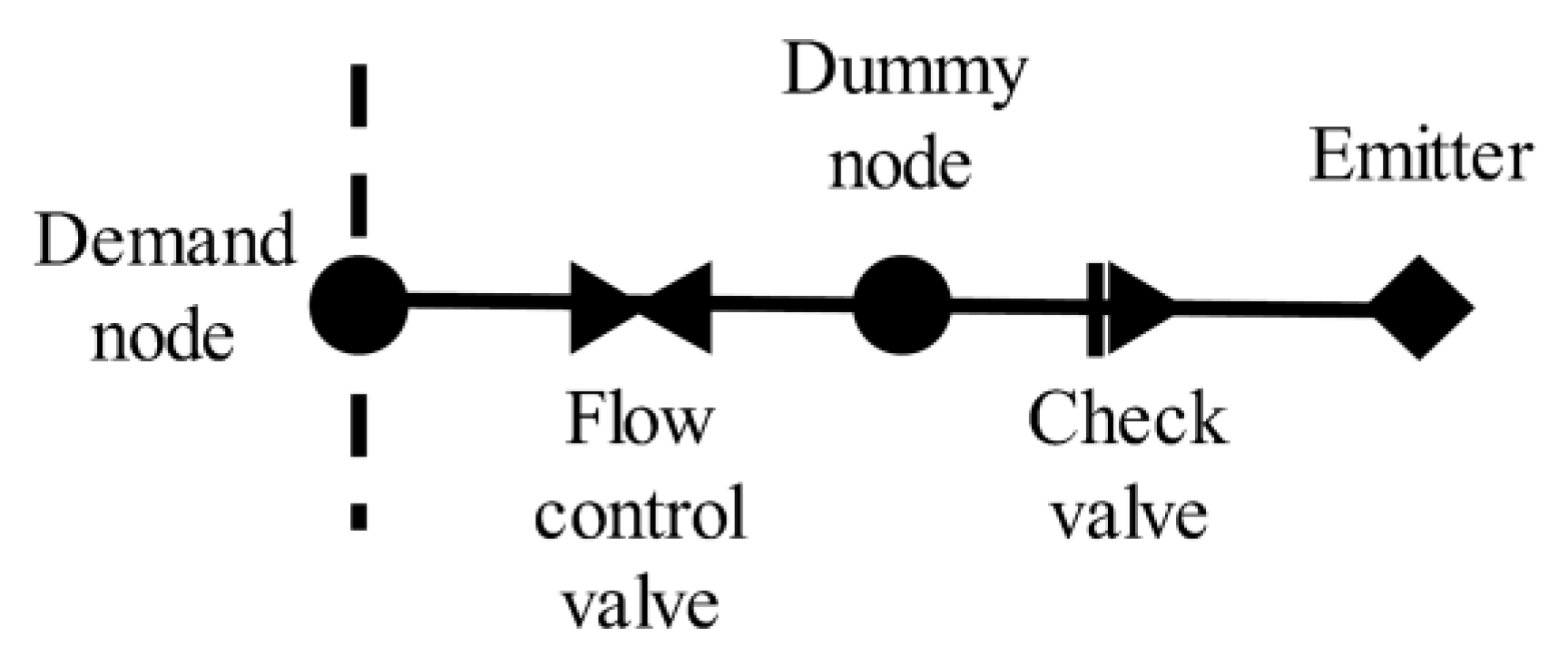
As shown in Figure 2, for each demand node, a flow control valve (FCV), a dummy node, a check valve (CV), and an emitter were added [28]. The emitter node was added to ensure the flow follows the exponent equation when ; the FCV ensures the maximum flow to the emitter is ; and the CV ensures the flow to emitter node is zero when .The dummy node was added to link the FCV and CV. During simulation, the base demand of both dummy node and demand node is set to zero, and the actual demand of emitter is considered as the real water consumption at the demand node.
2.4. Reliability Metrics
As mentioned in Section 1, two kinds of reliability metrics are calculated to evaluate the WDN’s functionality against FFEs to adequately supply both firefighting flow and original user demand under seismic damage.
2.4.1. Reliability Metrics to Quantify Reliability of Firefighting Water Supply
Predicating and modeling the firefighting demand in WDS is a very complex task, for ignition and spread of fire outbreaks are influenced by numerous factors such as weather, the number and the locations of ignitions, structural damage to the buildings, and the obstruction of roads, etc. In this study, the required firefighting flow rate was decided to be 90 L/s according to the National Code for Design of Outdoor Water Supply Engineering in China (GB50013-2006). The designed fire duration is set as 2 h according to the National Code for Design of Fire Water Supply and Fire Hydrant System in China due to lack of data.
In this study, the average serviceability of above-mentioned firefighting flows is presented as the WDN’s firefighting reliability metric. is defined as the ratio of available firefighting flow to the required firefighting flow at time step t.
where is the set of fire nodes at time step t; is firefighting flow rate available at node j in t time step; and is required firefighting flow rate at node j in the t time step.
2.4.2. Reliability Metrics to Quantify Functionality to Original Consumers’ Demand
In many previous studies, reliability metrics have been characterized as a derivate of the prevailing energy redundancy in the WDN [46,47,48,49]. The basic principle is that the WDN loses energy in the event of a fault (e.g., higher demand or component failure), and any available buffer energy that exceeds the minimum requirement will compensate for the potential energy loss associated with the fault [46]. Generally these metrics can be easily calculated without conducting hydraulic simulation under system failures which could be unrepresentative in some cases. In this study, system failures and additional load has already simulated by Monte Carlo simulations. Therefore, in this study, simulation result-based metrics, nodal serviceability [25], and system serviceability () [1,25,36] are chosen as the reliability metrics to quantify functionality to original consumers’ demand. In this study, the system seismic reliability () is defined as the ratio of the total supplied system demand to the total required system demand in time step t:
where is the system seismic serviceability in time step t; m is total number of demand nodes; is the available demand at node j in time step t; and is the required demand at node j in time step t.
where is the seismic serviceability of node j in time step t; is the available demand at node j in time step t; and is the required demand at node j in time step t.
2.5. Summary of Assumptions
A number of assumptions and simplifications were made in this study:
- (1)
- Restoration processes are not considered in this study because the simulation of restoration could greatly increase calculation time and the probability of generating abnormal solutions.
- (2)
- The interconnections with other lifeline networks (electric power, transportation, telecommunication, etc.) are not considered.
- (3)
- The expansion and spread of fire are not considered in this study.
- (4)
- The demand of nodes on damaged pipes is assumed as 70% of the original demand under seismic damage, according to National Code for Design of Outdoor Water Supply Engineering in China (GB50013-2006).
- (5)
- The required firefighting pressure is set as 20 m.
- (6)
- The supplied by fire tracks was ignored for calculation efficiency because their volume is small compared with the total required firefighting demand.
3. Study Network and Scenarios
3.1. Study Network
As shown in Figure 3, the developed simulation model was applied to a water supply network in MZ-city that is currently operating in Guangdong (GD) province, China. The geographical center of the city is shown in Figure 3, which was used to quantify the location and distance to epicenter. The MZ city network is a considerably a large WDN that serves a 52.2-km2 service area with a population of approximately 600,000. The system includes three sources, 2314 demand nodes, and 2451 pipes. At present, there are 9 known firefighting cistern exist in MZ city. If a node has a firefighting cistern, the volume of the required firefighting water of the node from WDN equal to the total firefighting water demand minus the volume of the fire cistern.
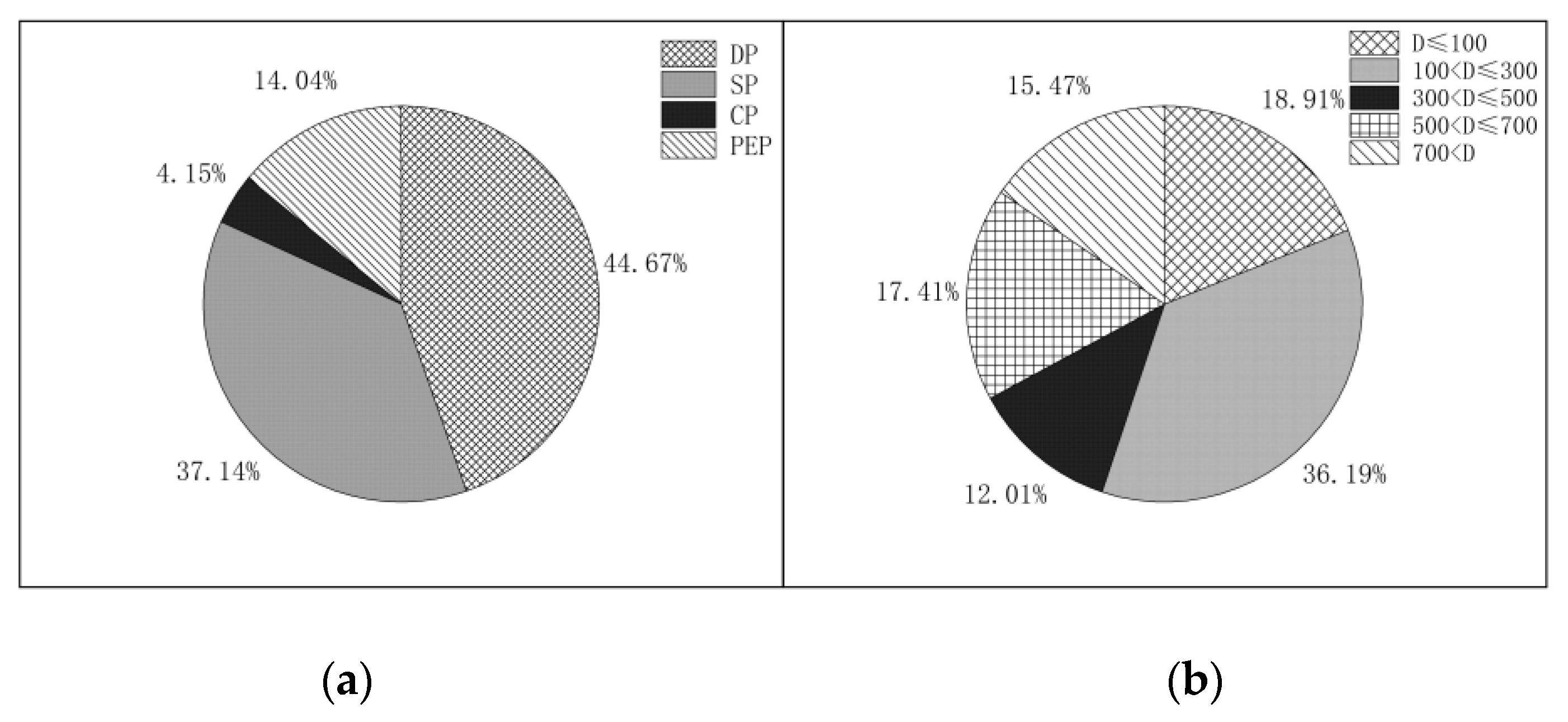
The MZ city network is a leak-suffering WDN for which the water loss rate is larger than 30%. The total length of transmission pipes with diameter larger than 80 mm is 311 km, with primarily looped-type connections. Pipelines in MZ city network range in diameter from 25 to 1000 mm and are made of different materials (cast iron pipes (CIPs), cement pipes (CPs), steel pipes (SPs), and the polyethylene pipe (PEP)), as illustrated in Figure 4.
3.2. Simulated Scenarios
As listed in Table 1, 8 artificially generated earthquake scenarios were investigated to evaluate the seismic reliability of the WDN of MZ City. The location of the epicenter was quantified by the distance and direction from the epicenter to the geographical center of the city. Because the spatial distribution of users and water sources in MZ city is relatively uniform, it was not necessary to simulate earthquakes from all directions. This study assumes that the earthquake occurred in the northwest direction of MZ city. The variation of earthquake severity was achieved by changing magnitude and distance.
According to the calculation results, the probability of component damage and fire caused by an earthquake with magnitude less than 5.0 is too small to have obvious impact on WDN. Thus, the minimum magnitude was set as 5.0. Meanwhile, earthquakes with magnitude larger than 7.0 would destroy large amount of the components to make the study meaningless.
In Scenario 1 and Scenario 2, the epicenter was set within the boundary of MZ city with magnitudes ranging from 5 to 7. Similarly, Scenario 3, Scenario 4, and Scenario 5 simulated seismic hazards that occurred in GD province with magnitudes ranging from 5 and 7. Scenarios 1–5 were established to investigate the effect of magnitude and epicenter location on WDN reliance. Scenario 6 is a typical seismic hazard with specific magnitude and epicenter location. Scenario 7 was generated assuming no component was damaged and Scenario 8 was built assuming no FFE happened during simulation.
4. Results and Discussion
4.1. Model Validation
The developed earthquake damage model was based on the historical data from ALA [16], and the spatial–temporal FFE model was based on historical data from main earthquakes in Japan [31], China [31], and the United States [15,32]. In order to ensure the accuracy of the model, the MZ city pipe network and users’ data were as detailed as possible for more accurate modeling results. Nevertheless, neither model was built considering MZ city’s historical seismic data, so they need verification of their accuracy in the study network. However, in the past 50 years, the total number of earthquakes with magnitude larger than 4.0 near Meizhou City was zero, which means that there are no reliable local earthquake damage and fire data to verify the proposed models.
Therefore, data from the Wenchuan earthquake (2008,China) [50,51] were used in this study to validate the proposed models, and were not used in model development. The data selected for verification work were from cities with a similar population and distribution of pipeline materials to MZ city. Table 2 showed the comparison between the average repair rate (RR) of seismic records in Wenchuan earthquake (2008, China) [50] and the average RR calculated by the model. Due to the lack of detailed data, all the correction factors in Equation (2) were assumed to be 1.0, and the average PGA was estimated from the average earthquake intensity recorded. Due to the lack of detailed data, it is difficult to make detailed and accurate estimates. However, the data of seismic record and model calculation still showed good agreement in Table 2.
Similarly, the reported fire outbreaks after the Wenchuan earthquake (2008, China) [51] are listed in Table 3. The building area was estimated according to the cities’ populations and building area per capita. Using the model proposed in Section 2.2, the model prediction value of quantity of FFEs was obtained and is shown in Table 3. The error of the proposed model is acceptable considering that the statistics recorded are not complete [51].
The reported fire occurred in the first three days after the earthquake, and most FFEs were concentrated in the first three hours after the earthquake, which is consistent with the prediction of the model.
4.2. Simulation Results of Compoent Failure and FFE Distribution
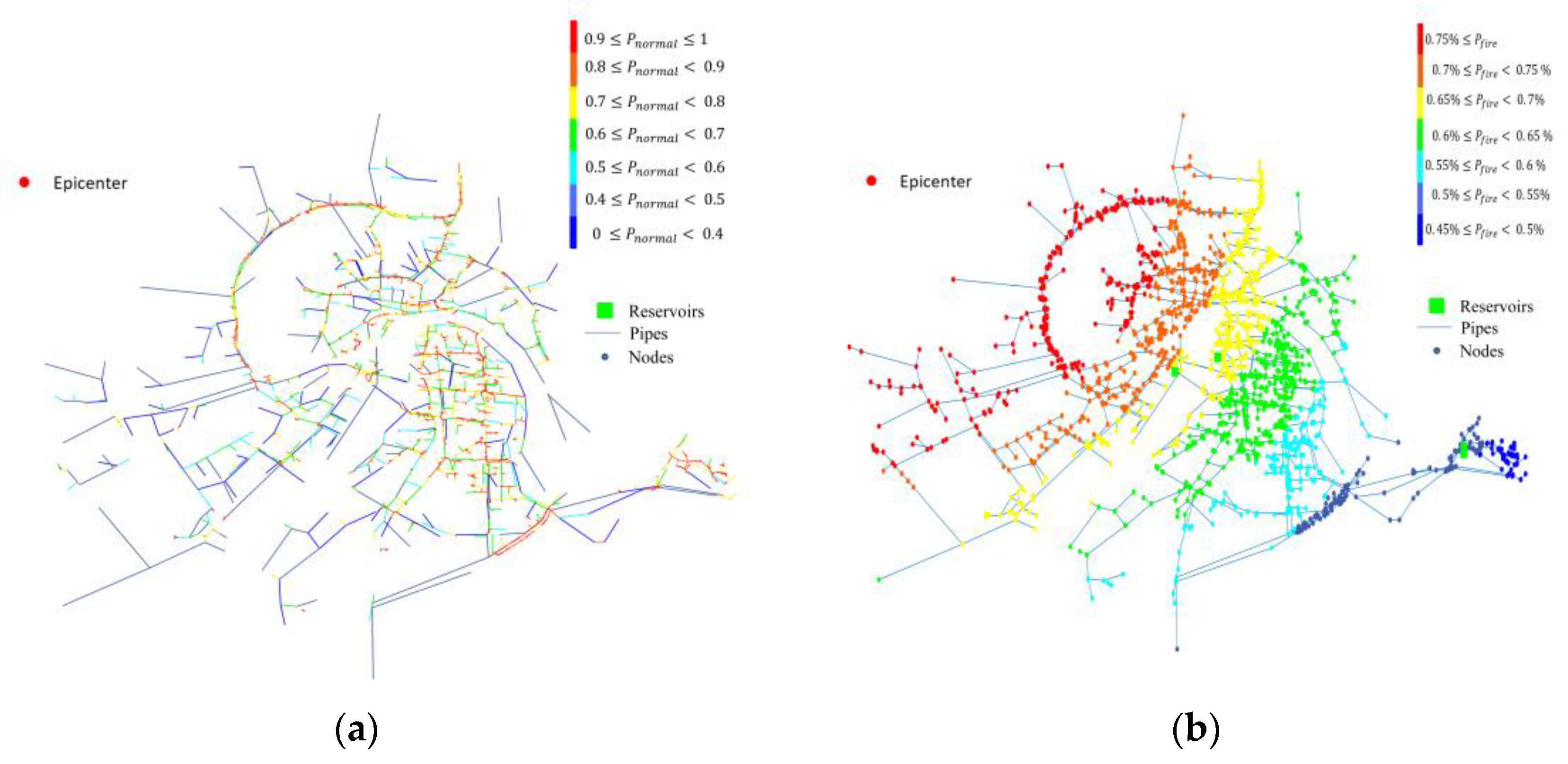
The component status (with leakage or breakage, or normal) was determined based on the PGA distribution and component attributes in each scenario. For example, the probability of pipes remaining undamaged in Scenario 1 (magnitude = 7) is shown in Figure 5a. It can be seen that the pipes near the reservoirs had a greater probability of remaining undamaged. This may due to the larger diameter of these pipes.
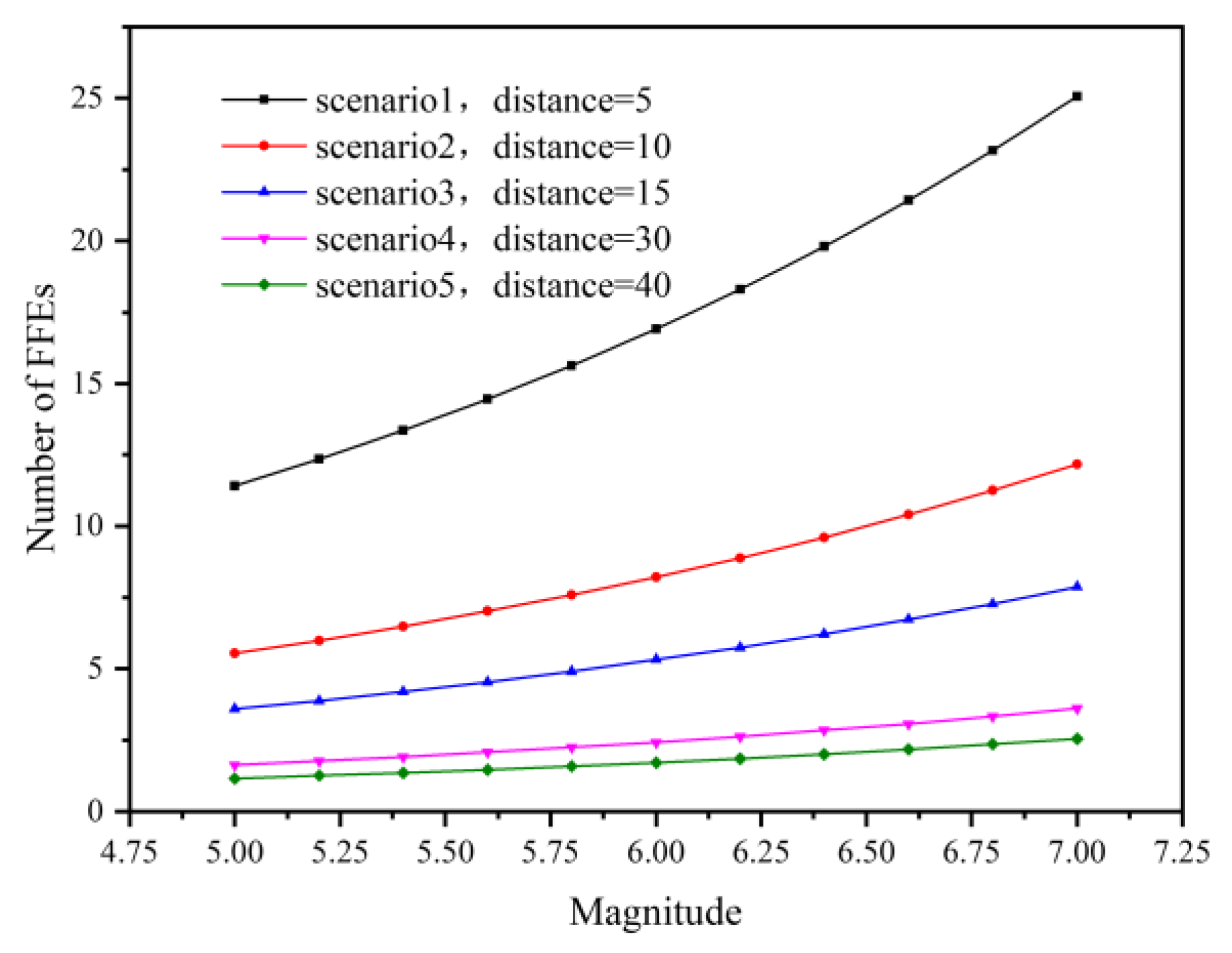
In addition to the seismic damage to WDN components shown in Table 1, FFE was simulated in each scenario except Scenario 8. The distribution of fire risk (probability of having one or more FFE) of each node in Scenario 1 (magnitude = 7) is shown in Figure 5b. The fire risk showed an obvious spatial distribution pattern. The node’s fire risk decreased as the distance from the epicenter increased. The relationship between average number of FFEs and the magnitude is shown in Figure 6. It can be seen that the number of FFEs increased approximately exponentially with magnitude. The maximum number of FFEs was 25.06 when the magnitude was 7.0 in Scenario 1. In Scenario 4 and Scenario 5, the number of fires was less than 3.6. In the case where the distance from the epicenter was larger than 40 km, even if the magnitude was as high as 7.0, the number of fires was very small (less than 1.1).
After the total number of FFEs in each scenario was decided, the temporal distribution of FFEs was calculated in each iteration of MCS. Taking temporal distribution of FFEs in Scenario 6 as an example, the number of fires per hour () decreased monotonously with time, as shown in Figure 7. The calculated total average number of FFEs in Scenario 6 and Scenario 7 was 16.09, and more than half of the fires occurred within 8 h after the earthquake. Because the after 8 h is relatively small, the calculated average serviceability of firefighting flows after first 8 h was more than 0.99 in most scenarios. Thus, average serviceability of firefighting flows in the first 8 h () was selected as the metric to evaluate the average performance of WDNs in supplying firefighting flow.
The temporal distribution of required firefighting flow is shown in Figure 6. As mentioned in Section 2.4.1, the designed fire duration was set to 2 h. Therefore, the peak of requirement of firefighting flow occurred in the second hour after the earthquake, because the firefighting flow was required to extinguish fires that occurred in both first and second hours. Note that the total consumption of the whole city was 853 L/s (regardless of firefighting water); the peak fire water consumption accounted for 38.7% of the total water consumption in Scenario 6.
4.3. System Reliability Metrics
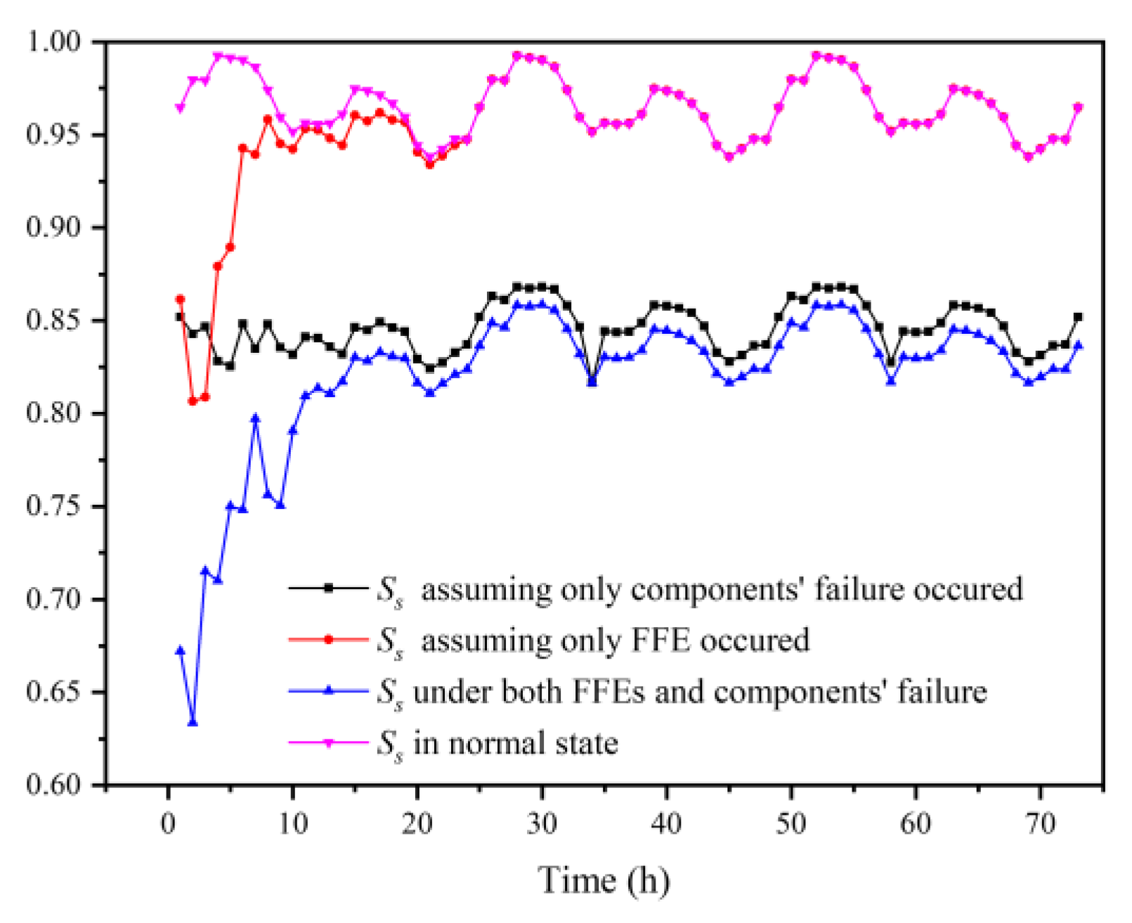
Table 4 summarizes the averaged simulation results of the predefined scenarios. It can be seen from Scenarios 1–5 that the average system serviceability () increased with the increases of the distance from the epicenter to the city’s geographical center. Scenario 1 was the worst scenario, with only 47.4 % of water successfully delivered to consumers. The minimum system serviceability (Ss) reached 0.3199 when the magnitude was 7.0 and the distance was 5.0 km. The maximum system serviceability was 0.9281 in Scenario 5, when the magnitude was 5.0 and the distance was 40 km. showed the same trend as Ss. Less than half of the firefighting water could be delivered in first 8 h in Scenario 1. Note that MZ city network is a leak-suffering WDN which is unable to fully satisfy consumer demand (average = 0.9653) even in a normal state and could not deliver adequate firefighting flow () without seismic damage (shown in Figure 8).
4.3.1. Seismic Reliability Evaluation for Original Demand
As analyzed in Section 4.2, the firefighting flow may account for a large part of the total water consumption, which could lead to a larger head loss. In this section, nodal serviceability () and system serviceability in Scenario 6 (with fire simulated) and Scenario 8 (no fire simulated) are shown as an example to quantify the functionality of MZ city network for original demand under the effect of both component failure and firefighting load.
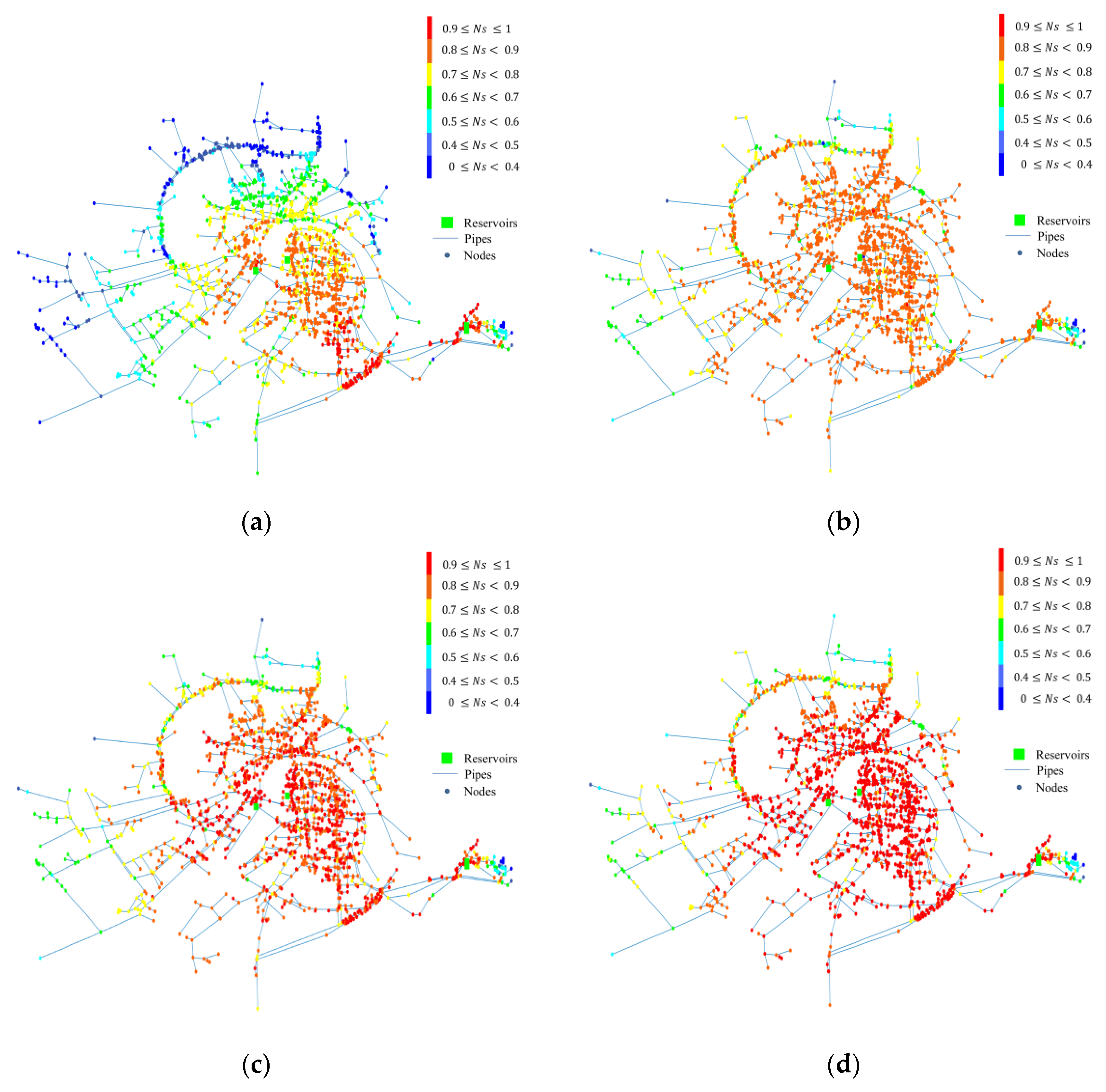
Figure 9a,b showed the distribution of nodal serviceability with peak firefighting flow (t = 2) in Scenario 6 and Scenario 8, respectively. It can be seen the system serviceability () reduced 24.7% because of the peak firefighting flow. The number of people without water supply increased from about 94,000 to about 220,000. Figure 9c,d showed the distribution of average nodal serviceability in scenario 6 and scenario 8, respectively. However, the average system serviceability reduced only about 3%. This may due to the low fire flow after 8 h was very small compared with leak flow.
Generally, the water supply network should have the ability to resist water consumption peak. For the study network, an only 38.7% additional increase of water consumption led to a 20% water shortage for users, which is unacceptable. Therefore, for MZ city network, the first goal is to repair and replace the old pipes, and increase the pipe diameter of the important pipes to improve the water supply capacity of MZ city network. The method proposed in this study can be used as a part of the decision aid tool for the planning of pipeline maintenance priority.
Figure 8 shows the trend of system serviceability () over time with the assumption that: (1) only component failure occurred (black line); (2) only FFE occurred (red line); (3) both FFE and component failure occurred (blue line); and (4) neither FFE nor component failure occurred (carmine line). It can be seen that firefighting flow had a significant effect on system serviceability only in a first 8 h after the earthquake. Since no restoration work was conducted in this study, it can be concluded that the increase of system serviceability (), assuming FFE occurred (red line in Figure 8) and both FFE and component failure occurred (blue line in Figure 8) in first 8 h, was due to the change of firefighting flows (shown in Figure 7). The decrease of system serviceability () in the first 8 h shows that the fire discharge is an essential reference variable in evaluating the seismic reliability of the pipe network.
The component failure decreased on average 12.3% of the system serviceability during 3 days. Compared with effect of component failure, FFE had lower influence on system serviceability, except for the first 8 h.
4.3.2. Seismic Reliability Evaluation for the System’s Firefighting Water Supply
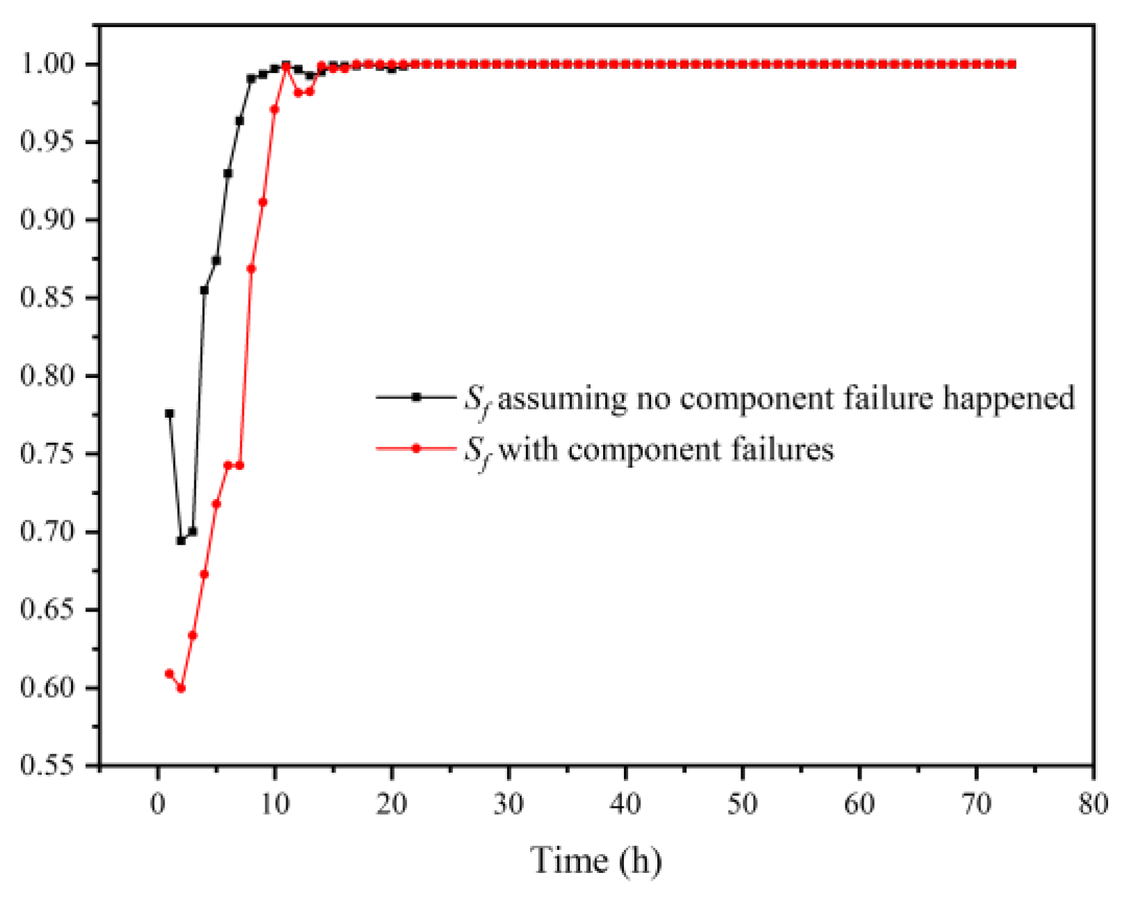
In this section, serviceability of firefighting flows in Scenario 6 (with component failure simulated) and Scenario 7 (no component failure simulated) is shown as an example to quantify the effect of component failure on reliability of MZ city network for firefighting flow. As shown in Figure 10, the minimum occurred when peak firefighting flow occurred (t = 2 h). The reduced on average by about 17.6% in the first 8 h. The average remained very close to 1 regardless of component failure due to the small required firefighting flow. Since no restoration work was conducted in this study, the increase of the serviceability of firefighting flows may due to the change of the firefighting flow itself.
It can be seen from Figure 8 and Figure 10 that the most obvious decrease of serviceability was due to the intensive firefighting flow that occurred in the first few hours. Therefore, in the process of WDN planning and design, it is necessary to ensure that there is sufficient fire water source for use in the first few hours after the earthquake. For example, the construction of fire cisterns and firefighting pipelines to natural water sources could be beneficial.
5. Conclusions
In this study, a multi-scenario simulation based model was developed to evaluate the reliability of WDNs for adequately supplying both original demand and firefighting flow under the effect of component failure and fire following earthquake (FFE). In the proposed model, hypothetical earthquakes were generated and seismic wave attenuation was calculated in PGA in each scenario. The component failure was simulated based on PGA and component attributes. The spatial distribution of FFEs was simulated by the Poisson distribution model and temporal distribution was simulated by Weibull distribution model. The component failures were simulated by closing pipes and adding emitters, and FFEs were simulated by adding additional demand of nodes in a hydraulic simulation model. For realistic hydraulic calculations, a PDA approach by adding artificial components on demand nodes was adopted. For each scenario, a Monte Carlo simulation with 10,000 iterations was conducted.
The model was applied was applied to a water supply network in MZ city that is currently operating in GD province, China. Eight seismic damage scenarios were generated with different epicenters and different magnitudes. Two types of reliability metrics were developed: the average serviceability of firefighting flows was presented as the WDN firefighting reliability metric, and nodal serviceability () and system serviceability () were chosen as the reliability metrics to quantify functionality to original demand. Several conclusions can be made from the results:
- (1)
- As the distance from the epicenter decreases and the magnitude increases, the total number of FFEs and the depth of failure increases.
- (2)
- The number of FFEs per hour decreased monotonically versus time. However, a period of time is needed to put out the fire. Thus, the firefighting flow may increase for a while before it decreases.
- (3)
- In a specific period of time after the earthquake, the influence of firefighting flow on system serviceability () is significant, while the average influence of firefighting flow is generally smaller than that of the component failure. Thus, replacement and new installation of pipes in WDNs are an effective way to improve reliability.
- (4)
- In a specific period of time after the earthquake, the component failures reduced average serviceability of firefighting flows significantly, while the average remained very close to 1 regardless of component failures after 10 h.
- (5)
- The minimum value of and occurred when peak firefighting flow occurred (t = 2 h in this study).
The proposed model quantified WDN performance under specific seismic damage and potential FFEs, and can be used for planning, design, and maintenance of WDNs. The results showed the most obvious decrease of serviceability was due to the large and intensive firefighting flow occurring in the first few hours. Thus, the construction of a reliable additional fire water source may effectively reduce fire damage and mitigate the WDN’s firefighting load after an earthquake. For example, more fire cisterns and firefighting pipelines to natural water sources could be beneficial. The method proposed in this study can be used as a part of a decision aid tool for the maintenance of pipes and the construction of fire cisterns and firefighting pipelines. This study has several limitations that future research should address. Post-earthquake actions such as optimal operation of pumps and valves and scheduling for pipe repairs are not considered in this study. In addition, the interdependence between different infrastructure systems (e.g., between electric power and water systems) could be explored to provide more meaningful results.
Author Contributions
Determination of the research content, Y.L., J.G., and H.Z.; methodology, Y.L.; provision of background data, L.D. and P.X.; model construction, programming and data acquisition, Y.L.; data analysis and model validation, Y.L.; writing—original draft preparation, Y.L.; writing—review and editing, J.G.; visualization, X.X.; project administration, J.G.; funding acquisition, J.G., H.Z., L.D., and P.X.
Funding
This study was financially supported by the National Natural Science Foundation of China (51778178); Natural Science Foundation of Heilongjiang (LH2019E044); the National Key Research and Development Project (2016YFC0802402, 2018YFC0406201-3); and the Shenzhen Science and Technology Program (JSGG20170823140113498).
Conflicts of Interest
The authors declare no conflict of interest.
References
- Yoo, D.G.; Jung, D.; Kang, D.; Kim, J.H. Seismic-Reliability-Based Optimal Layout of a Water Distribution Network. Water 2016, 8, 50. [Google Scholar] [CrossRef]
- Van Leuven, L.J. Water/Wastewater Infrastructure Security: Threats and Vulnerabilities. In Handbook of Water and Wastewater Systems Protection; Clark, R.M., Hakim, S., Ostfeld, A., Eds.; Springer: New York, NY, USA, 2011; pp. 27–46. [Google Scholar] [CrossRef]
- Jeon, S.-S.; O’Rourke, T.D. Northridge Earthquake Effects on Pipelines and Residential Buildings. Bull. Seismol. Soc. Am. 2005, 95, 294–318. [Google Scholar] [CrossRef]
- Takada, S.; Kuwata, Y. Human life saving lifelines and cost-effective design of an exclusive water supply system for fires following earthquakes. In Earthquake Resistant Engineering Structures Vi; Brebbia, C.A., Ed.; Wit Press/Computational Mechanics Publications: Southampton, UK, 2007; Volume 93, p. 319. [Google Scholar]
- Kuraoka, S.; Rainer, J.H. Damage to water distribution system caused by the 1995 Hyogo-ken Nanbu earthquake. Can. J. Civ. Eng. 1996, 23, 665–677. [Google Scholar] [CrossRef]
- Scawthorn, C.; O’Rourke, T.D.; Blackburn, E.T. The 1906 San Francisco earthquake and fire-enduring lessons for fire protection and water supply. Earthq. Spectra 2006, 22, S135–S158. [Google Scholar] [CrossRef]
- Moroi, T.; Takemura, M. Mortality estimation by causes of death due to the 1923 Kanto earthquake. J. Jpn. Assoc. Earthq. Eng. 2004, 4, 21–45. [Google Scholar] [CrossRef]
- Meng, F.; Fu, G.T.; Farmani, R.; Sweetapple, C.; Butler, D. Topological attributes of network resilience: A study in water distribution systems. Water Res. 2018, 143, 376–386. [Google Scholar] [CrossRef]
- Soldi, D.; Candelieri, A.; Archetti, F. Resilience and vulnerability in urban water distribution networks through network theory and hydraulic simulation. In Computing and Control for the Water Industry; Ulanicki, B., Kapelan, Z., Boxall, J., Eds.; Elsevier Science Bv: Amsterdam, The Netherlands, 2015; Volume 119, pp. 1259–1268. [Google Scholar]
- Diao, K.G.; Sweetapple, C.; Farmani, R.; Fu, G.T.; Ward, S.; Butler, D. Global resilience analysis of water distribution systems. Water Res. 2016, 106, 383–393. [Google Scholar] [CrossRef]
- Raad, D.N.; Sinske, A.N.; van Vuuren, J.H. Comparison of four reliability surrogate measures for water distribution systems design. Water Resour. Res. 2010, 46, 11. [Google Scholar] [CrossRef]
- Greco, R.; Di Nardo, A.; Santonastaso, G. Resilience and entropy as indices of robustness of water distribution networks. J. Hydroinform. 2012, 14, 761–771. [Google Scholar] [CrossRef]
- Piratla, K.R.; Ariaratnam, S.T. Performance Evaluation of Resilience Metrics for Water Distribution Pipeline Networks; Pipelines: Fort Worth, TX, USA, 2013; pp. 330–339. [Google Scholar] [CrossRef]
- Creaco, E.; Fortunato, A.; Franchini, M.; Mazzola, M.R. Comparison between entropy and resilience as indirect measures of reliability in the framework of water distribution network design. In Proceedings of the 12th International Conference on Computing and Control for the Water Industry, Ccwi2013, Perugia, Italy, 2–4 September 2013; Brunone, B., Giustolisi, O., Ferrante, M., Laucelli, D., Meniconi, S., Berardi, L., Campisano, A., Eds.; Elsevier Science Bv: Amsterdam, The Netherlands, 2014; Volume 70, pp. 379–388. [Google Scholar]
- Federal Emergency Management Agency (FEMA). HAZUS97 Technical Manual; FEMA: Washington, DC, USA, 1997.
- American Lifelines Alliance. Seismic Fragility Formulations for Water Systems Part 1 Guideline; American Lifeline Alliance: Washington, DC, USA, 2001. [Google Scholar]
- Fragiadakis, M.; Christodoulou, S.E.; Vamvatsikos, D. Reliability Assessment of Urban Water Distribution Networks Under Seismic Loads. Water Resour. Manag. 2013, 27, 3739–3764. [Google Scholar] [CrossRef]
- Shi, P. Seismic Response Modeling of Water Supply Systems. Ph.D. Thesis, Cornell University, Ithaca, NY, USA, 1 January 2006. [Google Scholar]
- Liu, G.Y.; Chung, L.L.; Yeh, C.H.; Wang, R.Z.; Chou, K.W.; Hung, H.Y.; Chen, S.A.; Chen, Z.H.; Yu, S.H. A Study on Pipeline Seismic Performance and System Post-Earthquake Response of Water Utilities (1/2); Technical Report MOEA-WRA-0990095; Water Resource Agency, MOEA: Taipei, Taiwan, 2010.
- Liu, G.Y.; Chung, L.L.; Huang, C.W.; Yeh, C.H.; Chou, K.W.; Hung, H.Y.; Chen, Z.H.; Chou, C.H.; Tsai, L.C. A Study on Pipeline Seismic Performance and System Post-Earthquake Response of Water Utilities (2/2); Technical Report MOEA-WRA-1000090; Water Resource Agency, MOEA: Taipei, Taiwan, 2011.
- GIRAFFE. GIRAFFE User’s Manual; School of Civil and Environmental Engineering, Cornell University: Ithaca, NY, USA, 2008. [Google Scholar]
- Rossman, L.A. EPANET 2: Users’ Manual; U.S. Environmental Protection Agency (EPA): Cincinnati, OH, USA, 2000.
- Shi, P.; O’Rourke, T.D.; Wang, Y. Simulation of earthquake water supply performance. In Proceedings of the 8th National Conference on Earthquake Engineering, San Francisco, CA, USA, 18–22 April 2006. [Google Scholar]
- Wang, Y.; O’Rourke, T.D. Characterizations of seismic risk in Los Angeles water supply system. In Proceedings of the 5th China-Japan-US Symposium on Lifeline Earthquake Engineering, Haikou, China, 26–28 November 2007. [Google Scholar]
- Yoo, D.G.; Jung, D.; Kang, D.; Kim, J.H.; Lansey, K. Seismic Hazard Assessment Model for Urban Water Supply Networks. J. Water Resour. Plan. Manag. 2016, 142. [Google Scholar] [CrossRef]
- Zhao, S.J.; Xiong, L.Y.; Rea, A.Z. A spatial-temporal stochastic simulation of fire outbreaks following earthquake based on GIS. J. Fire Sci. 2006, 24, 313–339. [Google Scholar] [CrossRef]
- Zolfaghari, M.R.; Peyghaleh, E.; Nasirzadeh, G. Fire Following Earthquake, Intra-structure Ignition Modeling. J. Fire Sci. 2009, 27, 45–79. [Google Scholar] [CrossRef]
- Sayyed, M.; Gupta, R.; Tanyimboh, T.T. Noniterative Application of EPANET for Pressure Dependent Modelling of Water Distribution Systems. Water Resour. Manag. 2015, 29, 3227–3242. [Google Scholar] [CrossRef]
- Davidson, R.A. Modeling post-earthquake fire ignitions using generalized linear (mixed) models. J. Infrastruct. Syst. 2009, 15, 351–360. [Google Scholar] [CrossRef]
- Himoto, K. Comparative Analysis of Post-Earthquake Fires in Japan from 1995 to 2017. Fire Technol. 2019, 55, 935–961. [Google Scholar] [CrossRef]
- Jie, L.; Guoqiang, L. A Research on the Prediction Model of Earthquake—Aroused Fire Disaster. Earthq. Res. China 1992, 78–84. (In Chinese) [Google Scholar]
- Elhami Khorasani, N.; Garlock, M.E.M. Overview of fire following earthquake: historical events and community responses. Int. J. Disaster Resilience Built Environ. 2017, 8, 158–174. [Google Scholar] [CrossRef]
- Github. KIOS-Reasearch/EPANET-Matlab-Toolkit. Available online: https://github.com/KIOSResearch/EPANET-Matlab-Toolkit (accessed on 29 January 2015).
- Pun, W.K.; Ambraseys, N.N. Earthquake Data Review and Seismic Hazard Analysis for the Hong-Kong Region. Earthq. Eng. Struct. Dyn. 1992, 21, 433–443. [Google Scholar] [CrossRef]
- Isoyama, R.; Ishida, E.; Yune, K.; Shirozu, T.; IWA. Seismic damage estimation procedure for water supply pipelines. In Anti-Seismic Measures on Water Supply; IWA Publishing: London, UK, 2000; Volume 18, pp. 63–68. [Google Scholar]
- Choi, J.; Yoo, D.G.; Kang, D. Post-Earthquake Restoration Simulation Model for Water Supply Networks. Sustainability 2018, 10, 3618. [Google Scholar] [CrossRef]
- Ai, S. Post-Earthquake Fires and Performance of Firefighting Activity in the Early Stage in the 1995 Great Hanshin-Awaji Earthquake. IFAC Proc. 1998, 31, 1–9. Available online: https://www.sciencedirect.com/science/article/pii/S1474667017384653?via%3Dihub (accessed on 30 November 2019).
- Fire Department of Kobe City. Fire Situation Following Hyogo-ken Nambu Earthquake in Kobe City; Tokyo Press: Kobe, Japan, 1996. (In Japanese) [Google Scholar]
- Song, J.; Li, J. Study on the Computer Simulation to Postearthquake Fire. Eng. Earthq. Prev. 1997, 3, 32–36. (In Chinese) [Google Scholar]
- Gupta, R.; Bhave, P.R. Comparison of methods for predicting deficient-network performance. J. Water Resour. Plan. Manag. 1996, 122, 214–217. [Google Scholar] [CrossRef]
- Tanyimboh, T.T.; Tabesh, M. Comparison of methods for predicting deficient-network performance. J. Water Resour. Plan. Manag. 1997, 123, 369–370. [Google Scholar] [CrossRef]
- Ang, W.K.; Jowitt, P.W. Solution for water distribution systems under pressure-deficient conditions. J. Water Resour. Plan. Manag. 2006, 132, 175–182. [Google Scholar] [CrossRef]
- Babu, K.S.J.; Mohan, S. Extended Period Simulation for Pressure-Deficient Water Distribution Network. J. Comput. Civ. Eng. 2012, 26, 498–505. [Google Scholar] [CrossRef]
- Bertola, P.; Nicolini, M. Evaluating reliability and efficiency of water distribution networks. Edited in: Efficient Management of Water Networks. Des. Rehabil. Tech. 2006, 17, 7–23. [Google Scholar]
- Mahmoud, H.A.; Savic, D.; Kapelan, Z. New Pressure-Driven Approach for Modeling Water Distribution Networks. J. Water Resour. Plan. Manag. 2017, 143, 11. [Google Scholar] [CrossRef]
- Bin Mahmoud, A.A.; Piratla, K.R. Comparative evaluation of resilience metrics for water distribution systems using a pressure driven demand-based reliability approach. J. Water Supply Res Technol.-Aqua 2018, 67, 517–530. [Google Scholar] [CrossRef]
- Todini, E. Looped water distribution networks design using a resilience index based heuristic approach. Urban Water 2000, 2, 115–122. [Google Scholar] [CrossRef]
- Prasad, T.D.; Park, N.-S. Multiobjective Genetic Algorithms for Design of Water Distribution Networks. J. Water Resour. Plan. Manag. 2004, 130, 73–82. [Google Scholar] [CrossRef]
- Jayaram, N.; Srinivasan, K. Performance-based optimal design and rehabilitation of water distribution networks using life cycle costing. Water Resour. Res. 2008, 44, 15. [Google Scholar] [CrossRef]
- Endong, G.; Xiangjian, W. Earthquake damage analysis of water supply pipeline in Wenchuan earthquake. In Proceedings of the Symposium on Earthquake Engineering and Earthquake Disaster Mitigation for the First Anniversary of Wenchuan Earthquake, Chengdu, China, 2009. (In Chinese). [Google Scholar]
- Jizong, G. Fires, the Neglected Secondary Disasters in the Wenchuan Earthquake. City Disaster Reduct. 2013, 18, 10–11. (In Chinese) [Google Scholar]
Figure 1.
Flowchart of the Proposed Reliability Evaluation Model. PGA: peak ground acceleration; PDD: pressure-dependent demand.
Figure 1.
Flowchart of the Proposed Reliability Evaluation Model. PGA: peak ground acceleration; PDD: pressure-dependent demand.

Figure 2.
The artificial components added to conduct pressure-dependent analysis (PDA).

Figure 3.
Location and overview of the water distribution network (WDN) of MZ city.

Figure 4.
The distribution of water supply pipelines (by length) grouped by (a) pipe material; (b) pipe diameter.
Figure 4.
The distribution of water supply pipelines (by length) grouped by (a) pipe material; (b) pipe diameter.

Figure 5.
(a) The distribution of probability for pipes to remain undamaged after earthquake in Scenario 1, magnitude = 7; (b) The distribution of probability of fire of each node.
Figure 5.
(a) The distribution of probability for pipes to remain undamaged after earthquake in Scenario 1, magnitude = 7; (b) The distribution of probability of fire of each node.

Figure 6.
The average number of FFEs versus magnitude in each scenario.

Figure 7.
The number of FFEs per hour (red bar) and the required firefighting flow (blue line) versus time.
Figure 7.
The number of FFEs per hour (red bar) and the required firefighting flow (blue line) versus time.

Figure 8.
The trend of system serviceability () versus time with the assumption that: (a) only component failure occurred (black line); (b) only FFE occurred (red line); (c) both FFE and component failure occurred (blue line); (d) neither FFE nor component failure occurred (carmine line).
Figure 8.
The trend of system serviceability () versus time with the assumption that: (a) only component failure occurred (black line); (b) only FFE occurred (red line); (c) both FFE and component failure occurred (blue line); (d) neither FFE nor component failure occurred (carmine line).

Figure 9.
The distribution of (a) nodal serviceability () in Scenario 6, t = 2 h, = 0.6339; (b) nodal serviceability () in Scenario 8, t = 2 h, = 0.8427; (c) average nodal serviceability () in Scenario 6, = 0.8196; (d) average nodal serviceability () in Scenario 8, = 0.8461.
Figure 9.
The distribution of (a) nodal serviceability () in Scenario 6, t = 2 h, = 0.6339; (b) nodal serviceability () in Scenario 8, t = 2 h, = 0.8427; (c) average nodal serviceability () in Scenario 6, = 0.8196; (d) average nodal serviceability () in Scenario 8, = 0.8461.

Figure 10.
Serviceability of firefighting flows versus time assuming no component failure occurred (black line) and with component failure (red line).
Figure 10.
Serviceability of firefighting flows versus time assuming no component failure occurred (black line) and with component failure (red line).


Table 1.
Reliability evaluation scenarios and simulation assumptions. FFE: fire following earthquake.
Table 1.
Reliability evaluation scenarios and simulation assumptions. FFE: fire following earthquake.
| Cases | Seismic hazard | Simulation Assumption | |||
|---|---|---|---|---|---|
| Location (Number of Simulations) | Distance to Center of MZ City | Magnitude | FFEs Are Simulated | Component Failure Is Simulated | |
| Scenario 1 | MZ city (11) | 5 | 5–7 | yes | yes |
| Scenario 2 | MZ city (11) | 10 | 5–7 | yes | yes |
| Scenario 3 | GD province (11) | 15 | 5–7 | yes | yes |
| Scenario 4 | GD province (11) | 30 | 5–7 | yes | yes |
| Scenario 5 | GD province (11) | 40 | 5–7 | yes | yes |
| Scenario 6 | GD province (1) | 20 | 6 | yes | yes |
| Scenario 7 | GD province (1) | 20 | 6 | yes | no |
| Scenario 8 | GD province (1) | 20 | 6 | no | yes |
Table 2.
Comparison between the average repair rate (RR) of seismic records in the Wenchuan earthquake (2008, China) and the average RR calculated by the model.
Table 2.
Comparison between the average repair rate (RR) of seismic records in the Wenchuan earthquake (2008, China) and the average RR calculated by the model.
| City Name | Estimated Average PGA/g | Reported RR (Number of Repairs/km Pipes) | Calculated RR by Model (Number of Repairs/km Pipes) |
|---|---|---|---|
| Mianyang City | 0.15 | 1.61 | 1.35 |
| Guangyuan City | 0.40 | 3.27 | 3.65 |
| Jiangyou City | 0.15 | 1.48 | 1.35 |
| Mianzhu City | 0.30 | 3.14 | 2.75 |
| Qingchuan City | 0.15 | 1.19 | 1.35 |
| Wenchuan City | 0.40 | 3.30 | 3.65 |
Table 3.
Comparison between the reported in Wenchuan earthquake (2008, China) and the average RR calculated by the model. FFE: fire following earthquake.
Table 3.
Comparison between the reported in Wenchuan earthquake (2008, China) and the average RR calculated by the model. FFE: fire following earthquake.
| City Name | Estimated Average PGA/g | Spatial Probability Density of FFE (Number of FFEs per 100,000 m2 Building Area) | Estimated Building Area | Reported Quantity of FFEs | Calculated Quantity of FFEs by Model |
|---|---|---|---|---|---|
| Deyang Prefecture Urban Area | 0.10 | 0.06405 | 2050 | 125 | 131.30 |
| Du Jiangyan Prefecture Urban Areas | 0.10 | 0.06405 | 1350 | 78 | 86.46 |
| Mianzhu City | 0.30 | 0.18375 | 143.75 | 11 | 14.71 |
Table 4.
System reliability metrics for seismic scenarios. : system serviceability.
| Cases | Reliability Metric | |||
|---|---|---|---|---|
| Average | Minimum (Corresponding Magnitude) | Maximum (Corresponding Magnitude) | ||
| Scenario 1 | 0.4740 | 0.3199 (7.0) | 0.6726 (5.0) | 0.4174 |
| Scenario 2 | 0.6443 | 0.5035 (7.0) | 0.7706 (5.0) | 0.5272 |
| Scenario 3 | 0.7059 | 0.6029 (7.0) | 0.7943 (5.0) | 0.6166 |
| Scenario 4 | 0.8518 | 0.7932 (7.0) | 0.8998 (5.0) | 0.7669 |
| Scenario 5 | 0.8926 | 0.8489 (7.0) | 0.9281 (5.0) | 0.8107 |
| Scenario 6 | 0.8196 | / | / | 0.6983 |
| Scenario 7 | 0.9530 | / | / | 0.8479 |
| Scenario 8 | 0.8461 | / | / | / |
© 2019 by the authors. Licensee MDPI, Basel, Switzerland. This article is an open access article distributed under the terms and conditions of the Creative Commons Attribution (CC BY) license (http://creativecommons.org/licenses/by/4.0/).
Share and Cite
MDPI and ACS Style
Li, Y.; Gao, J.; Zhang, H.; Deng, L.; Xin, P. Reliability Assessment Model of Water Distribution Networks against Fire Following Earthquake (FFE). Water 2019, 11, 2536. https://doi.org/10.3390/w11122536
AMA Style
Li Y, Gao J, Zhang H, Deng L, Xin P. Reliability Assessment Model of Water Distribution Networks against Fire Following Earthquake (FFE). Water. 2019; 11(12):2536. https://doi.org/10.3390/w11122536
Chicago/Turabian StyleLi, Yuanzhe, Jinliang Gao, Huaiyu Zhang, Liqun Deng, and Ping Xin. 2019. "Reliability Assessment Model of Water Distribution Networks against Fire Following Earthquake (FFE)" Water 11, no. 12: 2536. https://doi.org/10.3390/w11122536
Note that from the first issue of 2016, this journal uses article numbers instead of page numbers. See further details here.