Evaluation of GloFAS-Seasonal Forecasts for Cascade Reservoir Impoundment Operation in the Upper Yangtze River
by
 , ,
, ,
Kebing Chen
1, 
Shenglian Guo
1,*,
Jun Wang
1,
Pengcheng Qin
2,
Shaokun He
1,
Sirui Sun
3 and
Matin Rahnamay Naeini
4,* 1
State Key Laboratory of Water Resources and Hydropower Engineering Science, Wuhan University, Wuhan 430072, China
2
Wuhan Regional Climate Centre, Hubei Meteorology Bureau, Wuhan 430074, China
3
Middle Changjiang River Bureau of Hydrology and Water Resources Survey, Wuhan 430012, China
4
Center for Hydrometeorology and Remote Sensing (CHRS) & Department of Civil and Environmental Engineering, University of California, Irvine, CA 92697, USA
*
Authors to whom correspondence should be addressed.
Water 2019, 11(12), 2539; https://doi.org/10.3390/w11122539
Submission received: 1 November 2019
/
Revised: 24 November 2019
/
Accepted: 28 November 2019
/
Published: 1 December 2019
(This article belongs to the Special Issue Advances in Hydrologic Forecasts and Water Resources Management )
Abstract
:Standard impoundment operation rules (SIOR) are pre-defined guidelines for refilling reservoirs before the end of the wet season. The advancement and availability of the seasonal flow forecasts provide the opportunity for reservoir operators to use flexible and early impoundment operation rules (EIOR). These flexible impoundment rules can significantly improve water conservation, particularly during dry years. In this study, we investigate the potential application of seasonal streamflow forecasts for employing EIOR in the upper Yangtze River basin. We first define thresholds to determine the streamflow condition in September, which is an important period for decision-making in the basin, and then select the most suitable impoundment operation rules accordingly. The thresholds are used in a simulation–optimization model to evaluate different scenarios for EIOR and SIOR by multiple objectives. We measure the skill of the GloFAS-Seasonal forecast, an operational global seasonal river flow forecasting system, to predict streamflow condition according to the selected thresholds. The results show that: (1) the 20th and 30th percentiles of the historical September flow are suitable thresholds for evaluating the possibility of employing EIOR; (2) compared to climatological forecasts, GloFAS-Seasonal forecasts are skillful for predicting the streamflow condition according to the selected 20th and 30th percentile thresholds; and (3) during dry years, EIOR could improve the fullness storage rate by 5.63% and the annual average hydropower generation by 4.02%, without increasing the risk of flooding. GloFAS-Seasonal forecasts and early reservoir impoundment have the potential to enhance hydropower generation and water utilization.
1. Introduction
The rapid population and economic growth in recent decades, along with climate change and variability, impose more stress on water resources and cascade reservoir systems. Reservoirs, as one of the most important components of the hydrologic system, play a significant role as water supply by altering natural streamflow across space and time [1,2], while mitigating the effect of extreme events [3,4]. Conventionally, during wet season, reservoir operators release water preferentially for flood control [5,6] while storing water before the end of wet season to meet the demand for hydropower generation, navigation, and water supply. For full replenishment of storage, reservoir operators and academic researchers have highlighted the importance of reservoir impoundment operation and impoundment rules in several studies [7,8,9,10].
Reservoir operation rules are often used to provide guidelines for reservoir operators to determine the amount of controlled discharge. Among these rules, the reservoir impoundment rules are designed to refill the reservoir and raise the storage water level. The New York City rule [11] is among the early guidelines for reservoir impoundment and provides the probability of spills rather than the amount of spill to minimize the water shortage [12]. Since the development of the New York City rule, different types of reservoir impoundment operation rules have been developed and employed for various reservoir systems [7,13,14,15,16,17]. In the Yangtze River, which is one of the largest rivers in the world by discharge volume with huge reservoir storage capacity, the impoundment operation is complex and challenging. Water managers and stakeholders employ predefined impoundment rules for reservoir systems. These fixed rules, so-called standard impoundment operation rules (SIOR), are derived based on the historical flow records [7,9,18]. The SIOR is designed to reduce the flood control risk during the impoundment period. However, these fixed rules are unable to fully replenish the storage of the reservoir during dry years, which could lead to water shortage. On the contrary, flexible early impoundment operation rules (EIOR) allow the reservoir operators to start the impoundment process earlier and avoid unnecessary spills. However, employing EIOR requires information about the streamflow forecast to alleviate the risk of flooding.
The recent advancements of the meteorological and hydrological forecast systems provide an unprecedented opportunity for employing flexible operation rules rather than fixed ones for reservoir systems [19,20,21]. Combining seasonal meteorological forecasts with hydrological models at continental-scale has provided several continental-scale seasonal hydro-meteorological forecasting systems [22,23,24], such as the European Flood Awareness System [25], the Australian Government Bureau of Meteorology Seasonal Streamflow Forecasts [26], and the National Hydrologic Ensemble Forecast Service, USA [27]. Several studies have demonstrated that a skillful streamflow forecast can enhance the efficiency of water allocation systems to manage the trade-off between hydropower, irrigation, municipal, and environmental services [28,29,30,31]. The potential for employing seasonal forecast in the Yangtze River basin has been investigated in several research studies, mostly through statistical techniques [32,33,34]. However, the potential application of the available seasonal forecasts for reservoir impoundment operation is not well understood in the Yangtze River basin. In this study, we evaluate the global seasonal river flow forecasting system (GloFAS-Seasonal) developed by the European Centre for Medium-Range Weather Forecasts (ECMWF) [35] for reservoir impoundment in the upper Yangtze River basin.
We follow two steps for our evaluation. First, we investigate different streamflow thresholds to evaluate the possibility of employing EIOR. These thresholds can be considered as an indicator for the dry condition which has adverse effects on reservoir impoundment operation. To find these thresholds, we analyze multiple impoundment operation scenarios for EIOR and SIOR using a simulation–optimization model. We test different percentiles of historical streamflow as thresholds to find the impoundment rule curves for these scenarios. These rule curves are derived using the non-dominated sorting genetic algorithm-II (NSGA-II) [36] through a multi-objective optimization process. We then analyze the objective function values to select the most suitable thresholds for employing EIOR or SIOR. Second, we apply these thresholds to evaluate the skill of the GloFAS-Seasonal streamflow forecast for selecting EIOR or SIOR. When the streamflow forecast is below the selected threshold, it means a dry condition. Hence, the EIOR provides a longer impoundment period during this condition and a more suitable impoundment approach for water conservation. We employ different scores to show the skill of the GloFAS-Seasonal streamflow forecast to detect the streamflow condition according to selected thresholds.
The rest of the paper is organized as follows: In Section 2, after introducing the study area, we build a cascade reservoir impoundment model for reservoir early refill operation. Section 3 reviews the GloFAS-Seasonal forecasting system and explains different measures to evaluate the skill of the forecast for streamflow conditions. We demonstrate and discuss the results for the streamflow thresholds and performance of the GloFAS-Seasonal forecast in Section 4. Finally, we draw the conclusion in Section 5.
2. Cascade Reservoir Impoundment Model
2.1. Study Area
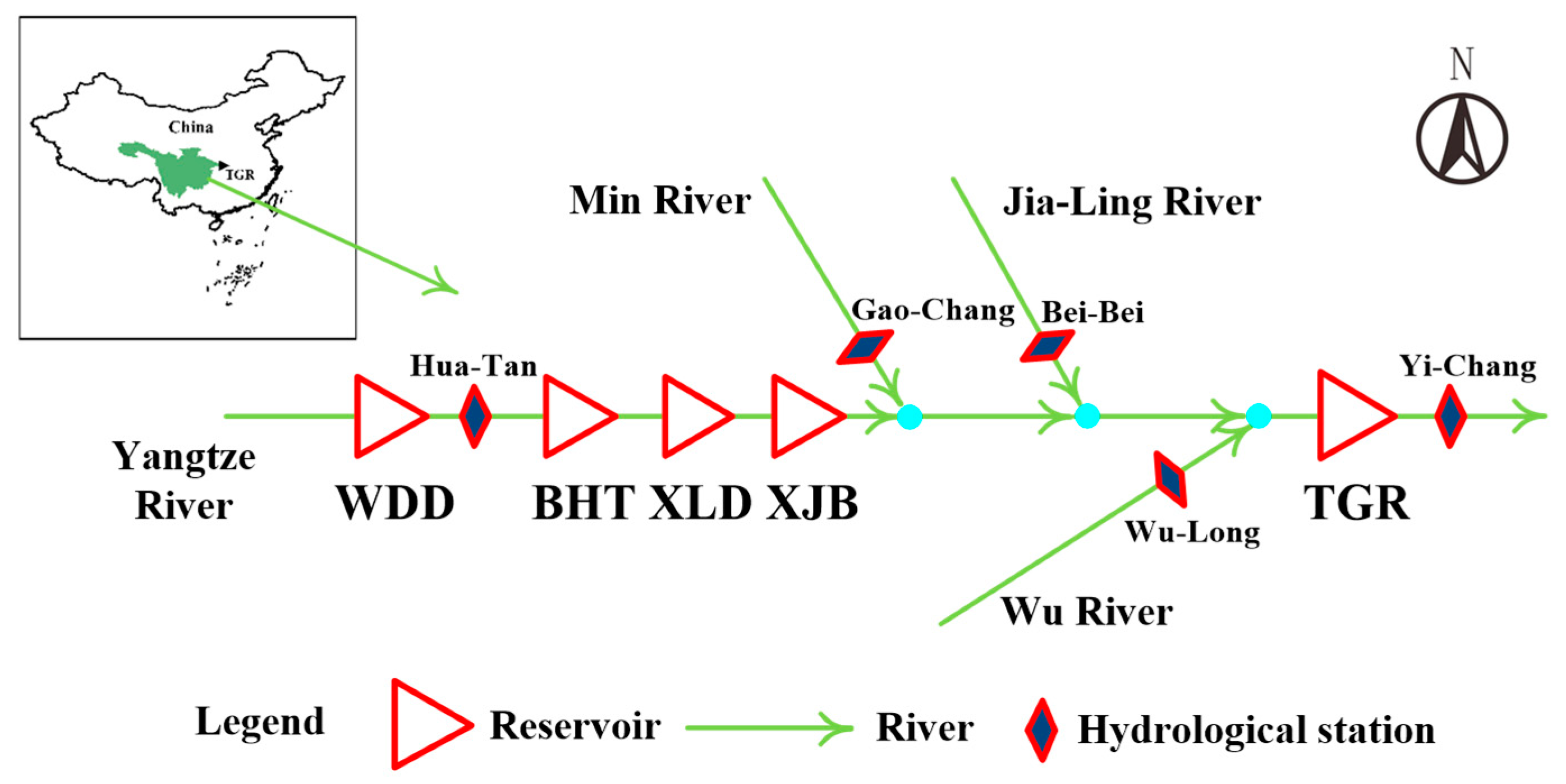
The Yangtze River, the longest river in Asia, flows 6300 km to the East China Sea with a total drainage area of 1.8 million km2 and has abundant hydropower resources. A series of cascade reservoirs have been constructed along the upper Yangtze River which provides a wide range of services including flood control, hydropower generation, water supply, as well as navigation. There are five cascade reservoirs in the upper Yangtze River, WDD (Wu-Dong-De), BHT (Bai-He-Tan), XLD (Xi-Luo-Du), XJB (Xiang-Jia-Ba), and TGR (Three Gorges Reservoir). These reservoirs, along with their characteristics, are listed in Table 1. There are no main tributaries between WDD and XJB reservoirs, while there are three main tributaries between XJB and TGR, Min River, Jia-Ling River, and Wu River. The inflow to WDD (QWDD) and TGR (QTGR) are derived from gauges at Hua-Tan and Yi-Chang hydrological stations by revivification, respectively. Figure 1 shows the sketch map of the cascade reservoirs, hydrological stations, and tributaries in the upper Yangtze River basin.
2.2. Impoundment Operation Rules for Cascade Reservoirs
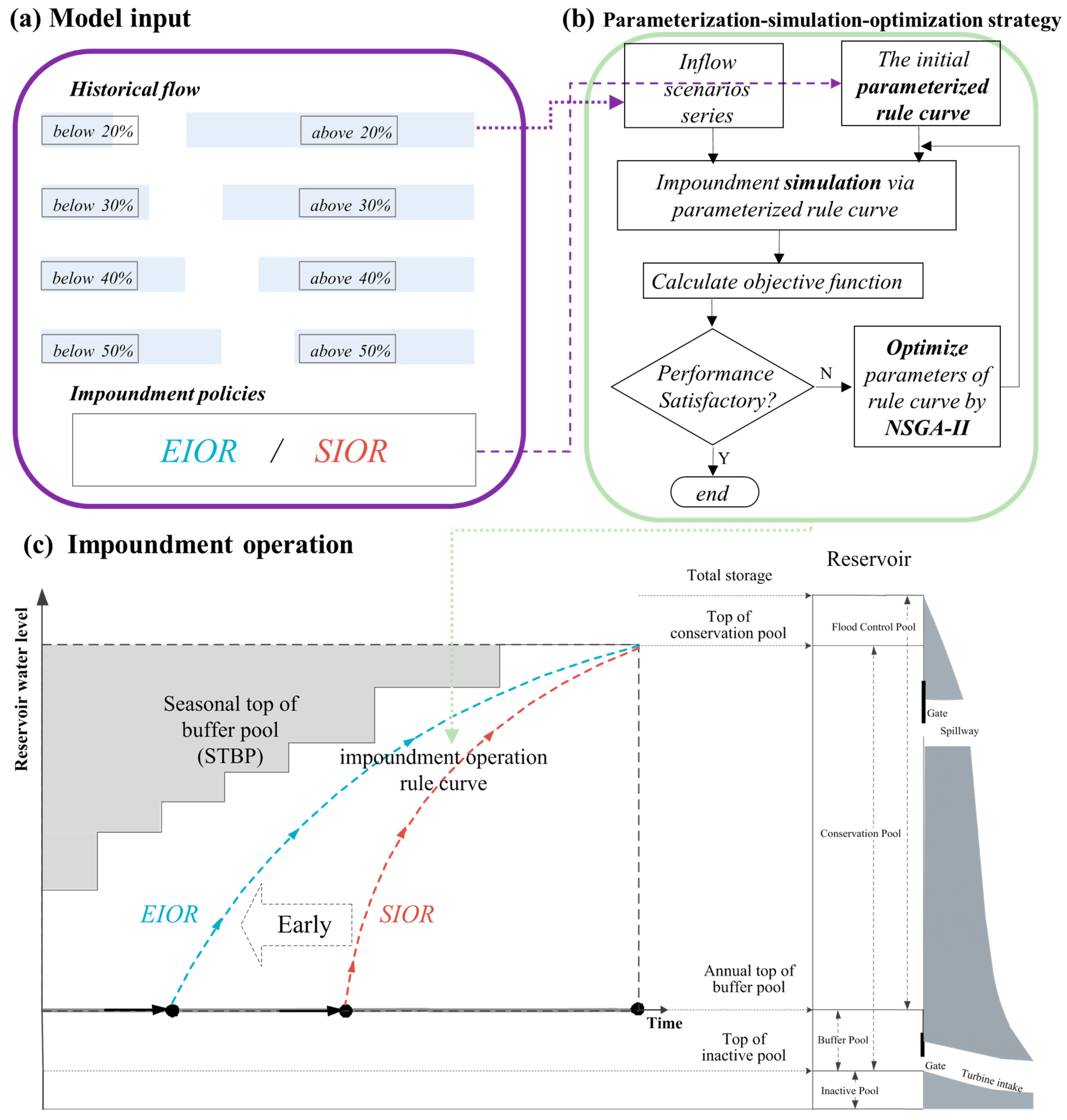
The impoundment operation rules are employed to refill reservoir storage during the impoundment period. The impoundment operation rules (Figure 2c) delineate trajectories to raise the water level from the annual top of buffer pool at the initial impoundment time to the top of conservation pool by the end of impoundment period. The SIOR derived from historical flow records initiates the impoundment operation at fixed predefined dates. However, the SIOR may fail to refill reservoir during the impoundment period in dry years. Hence, in low flow conditions and dry years, an early impoundment operation is more desirable to refill the storage capacity. Table 2 lists the potential time for employing early initial impoundment in the upper Yangtze River obtained from previous investigations [7,9]. We employ these initial dates along with the inflow conditions for the WDD and TGR reservoirs (QWDD and QTGR) to evaluate the possibility of an early impoundment for the cascade reservoirs.
Employing EIOR without considering the seasonal top of buffer pool (STBP) could increase the risk of flooding. Figure 2c shows the concept of the STBP and Table 3 lists the value of the STBP for selected reservoir (calculation method obtained from previous studies [7,9]). STBP is employed as the maximum water level to mitigate the risk of flooding for the impoundment period. We follow an iterative process to find the STBP for the reservoirs by evaluating the most extreme event. For further information for this process, please refer to [7,9]. We use the STBP in our model to control and assess the risk of flooding for the selected reservoirs.
According to Table 2, the impoundment process for most reservoirs starts before September. Hence, streamflow forecast data with 2-month lead time can be used in early August to evaluate the possibility of using EIOR. For this purpose, we define quantile-based thresholds based on historical September monthly inflow to the Wu-Dong-De and Three Gorges Reservoir (QWDD and QTGR). These thresholds are used to determine the streamflow condition to help decision-makers decide to use either EIOR or SIOR. For instance, if the September monthly QWDD is forecasted to be below the threshold percentile, EIOR is recommended as the suitable impoundment operation rule.
It is worth noting that, employing higher percentiles thresholds for inflow would increase the possibility of using EIOR. However, it also increases the risk of flooding. So, careful consideration should be devoted to the selection of these thresholds. Here, we examine four quantiles of historical monthly inflow in September, including 20, 30, 40, and 50-percentile (Figure 2a), for the QWDD and QTGR to select the best thresholds. For instance, considering the 20-percentile threshold of the historical monthly inflow in September, the observed inflow can fall into the above 20-percentile and below 20-percentile category. Then, we evaluate the potential benefit and risk for each of these thresholds by employing a cascade reservoirs impoundment simulation–optimization model under EIOR and SIOR scenarios. Since each of these thresholds divide the historical streamflow observation into two groups, we employ each group to find the impoundment rule curve separately. Hence, there are eight scenarios for the thresholds that need to be evaluated for each impoundment approach by the simulation–optimization model.
The reservoir simulation–optimization model is generally used to construct the rule curves by simulating the reservoir responses to predefined operating rules. Due to a large number of policies and constraints, mathematical optimization techniques can be used to identify the optimal operation rules by evaluating all possible alternatives [37]. The parameterization–simulation–optimization (PSO) approach is a popular and effective way of deriving optimal rule curves for cascade reservoirs [38]. Initially, PSO employs a linear rule curve (impoundment operation rule curve shown in Figure 2c), which connects the annual top of the buffer pool to the top of the conservation pool. It then employs a heuristic strategy to find the optimal rule curve according to predefined objective functions under possible inflow scenarios. Figure 2 shows the scheme of the PSO approach [39]. Finally, the objective function values of the PSO are employed to select the best threshold for reservoir impoundment decision-making.
Here, we employ PSO at a daily timescale to find the optimum rule curve for each threshold and scenario (Figure 2b). By optimizing the parameters of the rule curves for SIOR and EIOR, decision-makers can decide to employ EIOR or SIOR based on the obtained objective function values. The objective functions and the constraints for the impoundment operation employed in the PSO model are discussed in Section 2.3.1 and Section 2.3.2. In Section 2.4, we describe the NSGA-II algorithm employed for optimizing impoundment operation rule curve.
2.3. Objective Functions and Constrains
2.3.1. Objective Functions
Decision-makers rely on different criteria to make a comprehensive assessment of operation rules and address trade-offs among different users and services. In the Yangtze River, the goal of reservoir impoundment is to enhance water conservation in order to maximize hydropower generation and fullness storage rate, while minimizing the risk of flooding [7,18]. Hence, we employ objective functions that can measure the degree that these goals are achieved. These objectives are adopted from previous studies [7,18] and can be mathematically expressed as:
(1) Maximum hydropower generation (HG),
(2) Maximum fullness storage rate (FSR),
(3) Minimum flood control risk (R),
where
Rk = P (Water level > STBP) = Nrisk,k/N;
| M | the number of reservoirs; |
| N | the number of years for hydrological time series; |
| HGi,k | hydropower generation of the kth reservoir in the ith simulated year, kW·h |
| αk | the weight for fullness storage rate of the kth reservoir, calculated by the ratio about the total storage capacity of M reservoirs; |
| FSRi,k | fullness storage rate of the kth reservoir in the ith simulated year; |
| the storage capacity corresponding to the annual top of buffer pool of the kth reservoir, m3; | |
| the storage capacity corresponding to the top of conservation pool of the kth reservoir, m3; | |
| the highest storage during impoundment operation of the kth reservoir in the ith simulated year, m3; | |
| Rk | flood control risk of the kth reservoir; |
| Nrisk,k | the number of years when the water level exceeds STBP of the kth reservoir. |
2.3.2. Operation Constraints
In addition to the objective functions, the constraints of the reservoir system need to be specified for the optimization process. The following equality and inequality operational constraints need to be satisfied in the cascade reservoirs impoundment operation. Adopted from previous studies [7,18,40], the mathematical formulations of these constraints are as follows:
(1) Water balance equation,
(2) Reservoir capacity,
(3) Power generation,
(4) Reservoir discharge,
(5) Navigation,
where
| N | the number of years for hydrological time series; |
| T | total number of days during impoundment operation in the ith simulated year; |
| the kth reservoir storage at the beginning of the jth day in the ith simulated year, m3; | |
| the kth reservoir inflow on the jth day in the ith simulated year, m3/s; | |
| the water discharge of kth reservoir on the jth day in the ith simulated year, m3/s; | |
| the water discharge for hydropower generation of the kth reservoir on the jth day in the ith simulated year, m3/s; | |
| the spilled water discharge of the kth reservoir on the jth day in the ith simulated year, m3/s; | |
| Ak | the hydropower generation efficiency of the kth reservoir; |
| the average hydropower head of the kth reservoir on the jth day in the ith simulated year, m; | |
| the minimum power limits of the kth hydropower plant, kW; | |
| the maximum power limits of the kth hydropower plant, kW; | |
| the minimum water discharge for downstream of the kth reservoir, m3/s; | |
| the maximum water discharge for flood control safety in downstream of the kth reservoir, m3/s; | |
| ΔQk | the maximum water discharge fluctuation of the kth reservoir, m3/s; |
| the minimum water level at downstream of the kth dam site, m; | |
| the maximum water level at downstream of the kth dam site, m; | |
| the water level at downstream of kth dam site on the jth day in the ith simulated year, m; | |
| f(⋅) | the function provided by reservoir managers expressing the relationship between reservoir discharge and downstream water level. |
2.4. NSGA-II Optimization Algorithm
The nonlinearity of the reservoir systems, along with the existing constraints, require an effective optimization algorithm to solve these types of problems [41]. Here, we employ the non-dominated sorting genetic algorithm-II (NSGA-II), which is a robust multi-objective optimization algorithm [36], to derive the parameters of the rule curves. The NSGA-II algorithm has been applied to a wide range of complex multi-objective reservoir optimization and water resources management problems [18,38,42,43,44].
The NSGA-II algorithm has four parameters, including population size, generation number, crossover rate, and mutation rate, that need to be tuned by the user. Population size and generation number determine the effectiveness and efficiency of the algorithm and control the convergence speed to the optimal non-dominated solutions. Crossover and mutation rates control the ability of the algorithm to perform an effective search over the problem space [38,45]. In this study, the population size and the generation number were set to 50 and 200, respectively. These values are selected based on trial and error to obtain reasonable non-dominated solutions with acceptable simulation time. The crossover and mutation rates were empirically set to 0.9 and 0.1, respectively. The non-dominated solutions are used to evaluate the three objective functions for each threshold and each of the EIOR and SIOR scenarios.
3. Evaluation of GloFAS-Seasonal Forecasts
GloFAS-Seasonal forecasts combine the ECMWF’s latest seasonal meteorological forecasting system, SEAS5, and a river routing model, Lisflood, to provide streamflow forecasts at global scale [35]. This dataset provides weekly-averaged river flow with 4-month lead time. The first component of the GloFAS-Seasonal forecast is the meteorological input from SEAS5 which employs a data assimilation system along with a global circulation model. SEAS5 is executed once a month to produce seasonal weather forecasts with 7-month lead time. The second model component is a revised Hydrology Tiled ECMWF Scheme of Surface Exchanges over Land (HTESSEL) which computes the land surface response to atmospheric forcing and simulates the evolution of soil temperature, moisture content, and snowpack conditions through the forecast horizon to produce a corresponding forecast of surface and subsurface run-off [46]. The third model component is Lisflood which simulates the groundwater (subsurface water storage and transport) processes and routing of the water through the river network. While SEAS5 provides forecasts for the 7 months ahead, the GloFAS-Seasonal uses only the first 4 months and produces forecasts of river flow for the next 4 months. For more details on the forecast method, please refer to paper [35].
The GloFAS-Seasonal is a real-time forecast dataset which contains data from January 2018 and updates every month, with a total of 51 ensemble members. In order to evaluate the skill of the dataset, a set of retrospective seasonal forecasts for past dates, which are called reforecasts (also known as hindcasts), are available to compare with the historical observation streamflow. GloFAS-Seasonal reforecasts are available at http://www.globalfloods.eu/ and have 25 ensemble members from January 1981 to December 2017. In this study, GloFAS-Seasonal reforecasts at Hua-Tan and Yi-Chang hydrological stations in the Yangtze River are downloaded and analyzed. Also, the original weekly-averaged reforecasts are converted into monthly products for reservoir impoundment operation. Hence, monthly-averaged streamflow in September is obtained at the beginning of August with 2-month lead time (LM2).
We evaluate the GloFAS-Seasonal reforecasts to measure the capability of the dataset to predict the condition of the streamflow, i.e., the ability of the reforecast to predict that September monthly averaged flow falls below the selected thresholds which is defined in Section 2.1. Since seasonal climate is inherently probabilistic, seasonal forecasts should be evaluated probabilistically [47]. If each of the 25 ensemble members of the GloFAS-Seasonal reforecasts are equally likely, the proportion of ensemble members below each percentile threshold is calculated as the probability of the forecast. In addition, the percentile thresholds are calculated separately for historical observed and reforecast data [48]. This approach takes into account the systematic additive error (bias) of the reforecast data, hence further bias adjustment for the reforecast data is not required [48,49].
The conversion of raw ensemble members to forecast probabilities enables us to validate GloFAS-Seasonal reforecasts by using probabilistic forecasts verification measures. Here, we employ multiple metrics for our evaluation. These metrics include: I) discrimination, ability of the forecast to discriminate among observations; II) skill, the relative accuracy of the forecast over a reference forecast; III) reliability, the agreement between forecast probability and mean observed frequency; IV) resolution, the ability of the forecast to resolve the set of sample events into subsets; and V) sharpness, the tendency to forecast probabilities near 0 or 1. These metrics are briefly discussed here. Interested readers can refer to https://www.cawcr.gov.au/projects/verification/ for further details.
3.1. Discrimination
To assess the potential application of GloFAS-Seasonal forecasts for the prediction of the streamflow condition, the relative operating characteristic (ROC) curve, a measure of discrimination [50], is calculated for the selected thresholds. If the forecasts indicate that flow will be below threshold, which means a dry and unfavorable condition for reservoir impoundment operation, then a warning is issued. The forecasts are converted into a binary (e.g., “yes” or “no”) format depending on whether a warning has been issued or not issued. Then the ROC curve is plotted based on hit rate (HR) and false-alarm rate (FAR) of the forecast for streamflow condition. The HR and FAR can be calculated by Equation (12):
where h refers to a correct warning (hit), m refers to a missed warning, f refers to a false warning, and r correct no warning detection.
The area under the ROC curve (referred as AUC) is then calculated, which is used to measure whether the forecast is informative for decision-making. Most of the time, the ROC curve does not clearly indicate the accuracy of forecast. As a numerical value, it is more intuitive to use the AUC value as the evaluation standard. The larger the AUC value, the more skillful the forecast is. The value of the AUC ranges from 0 to 1. If the AUC is equal to 0.5, it indicates that forecasts are consistent with the random guess and provides no information. Generally, when the AUC value is greater than 0.6, the seasonal forecast can be regarded as useful [25,35].
3.2. Skill
Skill implies information about the relative accuracy of the forecast according to a reference forecast. The reference forecast is generally an unskilled forecast such as random chance, persistence, or climatology. To assess the skill of GloFAS-Seasonal reforecasts, we compare the reforecasts with climatology [51], an ensemble of observed flows, and use the ROC skill score (ROCSS), which has been used in previous studies for the verification of seasonal forecasts [52]. ROCSS is computed as follows:
where AUCfc refers to the AUC value of reforecasts and AUCcm refers to the AUC value of climatological forecasts. ROCSS of one means a perfect forecasting system; ROCSS of zero indicates no improvement over the climatology.
3.3. Reliability, Resolution, and Sharpness
For assessing the reliability of forecasts, the reliability diagram is used here, where X and Y axes represent the forecast probability and the observed frequency of the future below the streamflow threshold, respectively. When the forecast probability and the observed frequency are equal, the reliability of forecasts is perfect. For example, if an event will occur with a forecast probability of 70%, then, on average, the event should occur on 70% of the occasions that this forecast is made. So, reliability is indicated by the proximity of the plotted curve to the diagonal. If the plotted curve lies below the diagonal, this indicates over-estimation (forecast probabilities are too high); curve above the diagonal indicates under-estimation (forecast probabilities are too low).
The climatological average can produce high reliability, but it lacks information for practice. In theory, we are interested in probability forecast systems which give a forecast probability that deviates from the climatological average and approaches 0% or 100% while maintaining a high level of reliability [35]. So, the reliability diagram can also be used to assess the resolution of forecasts. Forecasts that discriminate between events and non-events are said to have a resolution (a forecast of climatological average, a curve lying on or near the horizontal line would have no resolution). For assessing the sharpness of forecasts, the reliability diagram is usually accompanied by a histogram. If the histogram is U-shaped, then the frequency of forecasts approaches 0% and 100% and the forecast system sharpness is well. Forecasts with no or low sharpness will show a peak in the forecast frequency near the climatological average.
4. Results and Discussion
4.1. The Selected Thresholds
As the first step of our evaluation, we select thresholds to evaluate the streamflow condition for impoundment operation. The Changjiang (Yangtze River) Water Resources Commission (CWRC) provides daily inflow and discharge data series for the selected five reservoirs and streamflow for adjacent gauges at hydrological stations, which covers the whole impoundment operation period from 1 August to 31 October (92 days) for 1950–2015 (66 years). We use 20, 30, 40, and 50-percentile of historical inflow as thresholds to determine the inflow condition in September according to the monthly-averaged inflow (QWDD and QTGR). For example, the 20-percentile historical average inflow in September divides data into two groups where one group (above 20-percentile in Figure 2a) includes 53 years of data and the other group (below 20-percentile in Figure 2a) has 13 years of data. Therefore, we get two scenarios for these thresholds, one above and one below each threshold. By this approach, we get 16 different flow scenario groups (two QWDD or QTGR × four quantiles × two groups for each quantile).
These scenarios are evaluated independently along with the EIOR and SIOR by the PSO approach. Since the population size for the NSGA-II algorithm is set to 50, the algorithm provides 50 Pareto-optimal solutions (non-dominated solutions). Since there are three objective functions for each scenario and considering the multi-purpose nature of these reservoirs, a single value cannot be reported as the best answer from these 50 Pareto-optimal solutions. Therefore, we average the objective function of the 50 Pareto-optimal solutions as a potential benefit and risk in response to this combination of historical flow group and impoundment rules. For 16 different groups and two operation rules, the averaged three objective functions of 50 Pareto-optimal solutions are shown in Table 4. Comparing these 16 different scenarios, we can see that the HG and FSR values are improved by employing larger thresholds. This improvement is due to the increase in streamflow and reservoirs storage in September from the lowest, below 20-percentile, to the highest, above 50-percentile, threshold. It is clearly shown that low flow in September has an adverse impact on impoundment operation.
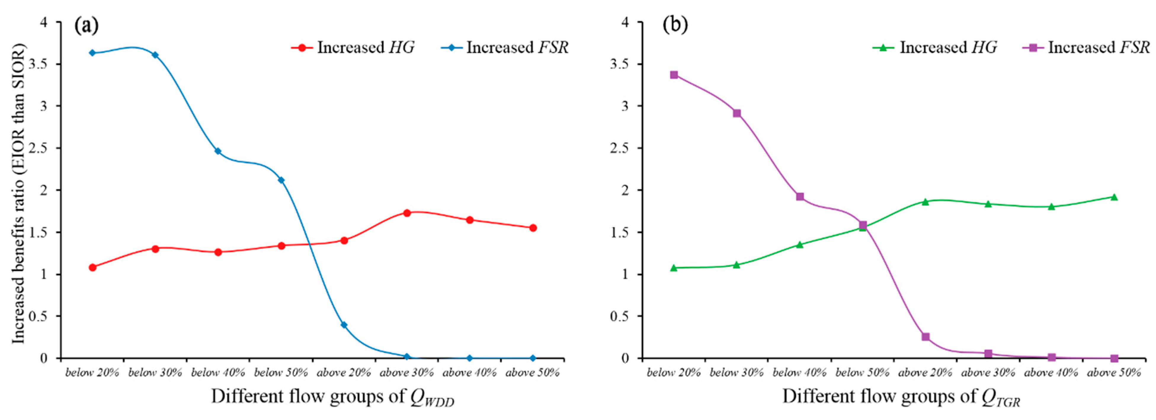
Comparing EIOR with SIOR for cascade reservoirs, the EIOR improves the HG and FSR from the flow group below 20% to below 40% for both of QWDD and QTGR without affecting the risk of flooding. We employ these results to select the most suitable threshold among these 16 scenarios for our analysis. Figure 3 shows the relationship between increased benefit ratio and different flow groups of QWDD and QTGR. According to Figure 3, HG is less affected by the selected thresholds. On the contrary, FSR values are decreased by increasing the threshold or inflow. For the group below the 20-percentile and below the 30-percentile, the FSRs of the proposed EIOR are increased significantly around or above 3% in comparison to the SIOR, without increasing the risk of flooding. Hence, we select the 20-percentile and 30-percentile as the thresholds for our study, as their performance is superior to others. In early August, we use these thresholds to evaluate the performance of the GloFAS-Seasonal in predicting the streamflow condition for QWDD and QTGR next month.
4.2. Evaluation of GloFAS-Seasonal Reforecasts
GloFAS-Seasonal reforecasts are evaluated using adjusted historical river flow data at the Hua-Tan and Yi-Chang hydrologic stations in the Yangtze River. GloFAS-Seasonal reforecasts represent natural flow and do not consider any reservoir routing. The CWRC provides monthly averaged historical flow records which have been adjusted to represent the natural flow. These adjusted historical natural streamflow timeseries span over thirty years (1981–2013). So, GloFAS-Seasonal reforecasts are evaluated over the same 33-year period. Since the impoundment operation starts before September, we investigate the GloFAS-Seasonal reforecasts on 1 August (2-month lead, LM2) to evaluate the potential for employing EIOR. We also investigate the 1-month lead, LM1, on 1 September to evaluate the performance of GloFAS-Seasonal for different lead times.
4.2.1. AUC Values
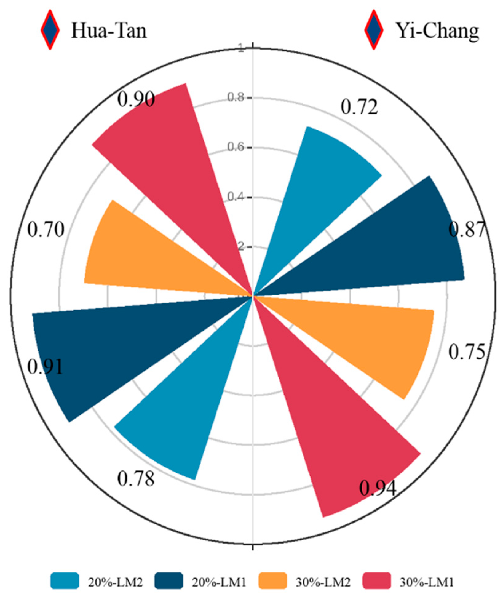
In order to compare AUC values for different stations, lead times, and thresholds, we employ the Nightingale’s Rose chart. This chart is suitable to visually evaluate the evident differences between various categorical data. The results are shown in Figure 4, and it is clearly shown that all AUC values are greater than 0.6, which means that the forecasts can be regarded as informative and have the ability to predict the streamflow condition (whether streamflow is below the threshold or not). Besides, the AUC values exhibit a decline from the LM1 (around 0.9) to the LM2 (below 0.8) as expected.
For different stations and thresholds, AUC values of forecasts vary more significantly with lead times. So, the discrimination of GloFAS-Seasonal reforecasts is relatively stable over space in the upper Yangtze River. Moreover, an interesting finding is that the performance of thresholds varies for hydrological stations. For Hua-Tan, the 20-percentile has the best performance, whereas the 30-percentile for the Yi-Chang station. This emphasizes that a spatial evaluation of thresholds is necessary for the Yangtze River to find the best thresholds for employing the GloFAS-Seasonal forecast at the basin.
4.2.2. ROCSS Values
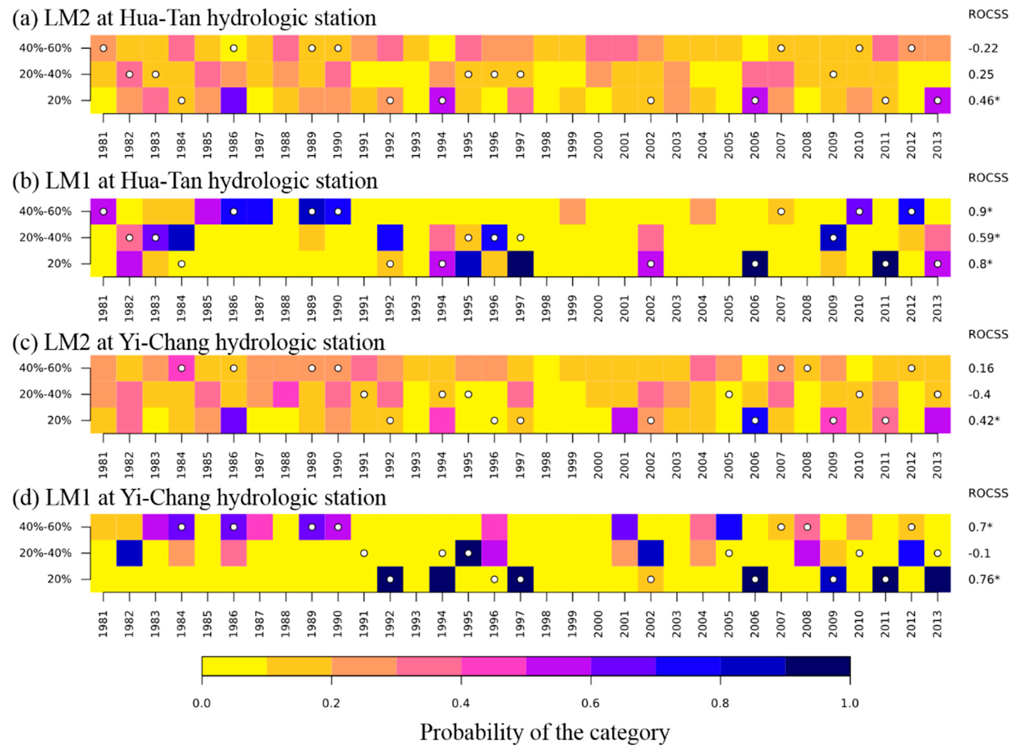
Tercile plots are designed to show the performance of a forecast system at different periods [53]. Here, we employ these plots to compare reforecast probabilities (color coded from light to dark color for lower to higher probability) for different threshold events with the observed condition (white dots). We defined three different categories of threshold events for our comparison. Since low flow condition leads to employing the EIOR, we only employ 0–20%, 20–40%, and 40–60% quantiles of the streamflow data to evaluate the performance of GloFAS-Seasonal reforecasts for predicting the correct flow condition. However, the evaluation can be done for other flow ranges based on the selected thresholds. ROCSS values for each quantile is shown on the right axis for comparison. Significant values of ROCSS with a 95% confidence are marked with an asterisk for statistical evaluation.
Results show that for GloFAS-Seasonal reforecasts below 20%, the ROCSS exhibit a decline in skill from the LM1 (0.8 and 0.76) to the LM2 (0.46 and 0.42) for both Hua-Tan and Yi-Chang hydrological stations. However, skills (ROCSS greater than 0) still prevail in the LM2 and are marked with asterisks, which means that forecasts of LM2 are better than climatology. Furthermore, forecast sharpness is also evident in this tercile plot. The darker the color of the square, the better the sharpness of that probabilistic forecasts is. Forecasts for both LM1 and LM2 exhibit sharpness, although the sharpness is higher for LM1, which is indicated by the colors of the squares in Figure 5.
According to Figure 5, the streamflow condition for the Hua-Tan hydrological station is below the 20-percentile in seven years, among which the forecast predicted the highest probability for five and three of these years by LM1 and LM2, respectively. For the Yi-Chang hydrological station, the number of years with streamflow below the 20-percentile is seven, out of which GloFAS-Seasonal reforecasts with LM1 and LM2 predicted the highest probability for five and three of these years, respectively. Consistent with the results of AUC, although LM1 shows better performance with shorter lead time, aiming at reservoir impoundment operation, GloFAS-Seasonal reforecasts with 2-month lead time (LM2) are still informative. Further, compared with the LM1, LM2 still has a lot of potential improvement in the future, which depends on developing the seasonal climate prediction. A similar analysis can be performed for the 30-percentile threshold with other ranges.
4.2.3. Reliability Diagram
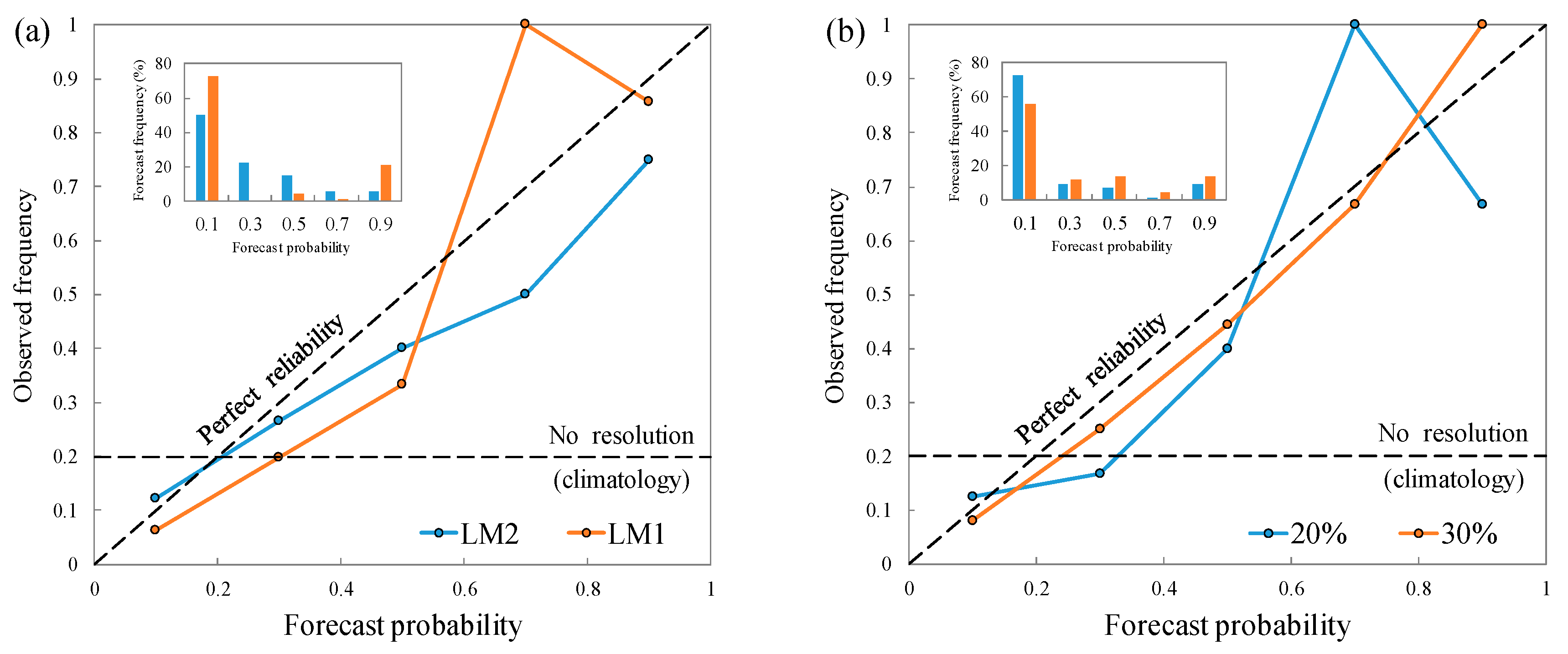
Similar to ROC calculations, the reliability is assessed for both the 20-percentile and 30-percentile threshold. Due to the limit number of samples, the range of forecast probabilities is divided into five bins (for every 20% from 0% to 100%) rather than ten bins in order to avoid sparseness of the probability categories. Since GloFAS-Seasonal reforecasts have similar performance at hydrological stations, reliability diagrams are only presented for Yi-Chang hydrologic station here. Figure 6 shows the effect of (a) the lead time (LM1 and LM2) and (b) the threshold (20-percentile and 30-percentile) on reliability by combining the contingency table for thresholds and lead times, respectively.
Figure 6a shows that forecasts have more reliability than climatology, regardless of the lead time. It is worth noting that the observed frequency is unrealistically equal to 1 for 60–80% and the LM1 due to sampling limitations rather than necessarily true deviations from reliability [54]. Overall, the reliability appears to be slightly better for forecasts of LM2 than LM1. The forecast data for both LM2 and LM1 exhibit sharpness, which means that forecast probabilities are more informative than climatology. Similar behavior is observed for the 60–80% bin in Figure 6b, because of the limited number of samples. Figure 6b shows that the reliability of the 30-percentile threshold is better than the 20-percentile. In contrast to reliability, sharpness is better for forecasts of the 20-percentile rather than the 30-percentile threshold. Differences in reliability and sharpness can be explained by the limited number of samples. So, the performance of the two selected thresholds is close and hard to distinguish.
Due to most dots laying below the diagonal, Figure 6 suggests that in general, GloFAS-Seasonal reforecasts have a tendency to over-estimate the likelihood of a below percentile streamflow condition, which is a common situation for seasonal forecasting [55]. This conclusion is consistent with the reliability diagram of GloFAS-Seasonal reforcasts aggregated across all observation stations globally [35], and reflects the characteristics of the GloFAS-Seasonal forecasting system. However, with respect to the impoundment of the reservoirs, it is more favorable to over-estimate the below threshold conditions rather than under-estimating. The reservoir operators could employ GloFAS-Seasonal forecasts for decision-making for the early impoundment operation, while control the risk of flooding through short-term hydrological forecasting in real-time operation.
4.3. Specific Analysis and Benefits of the EIOR
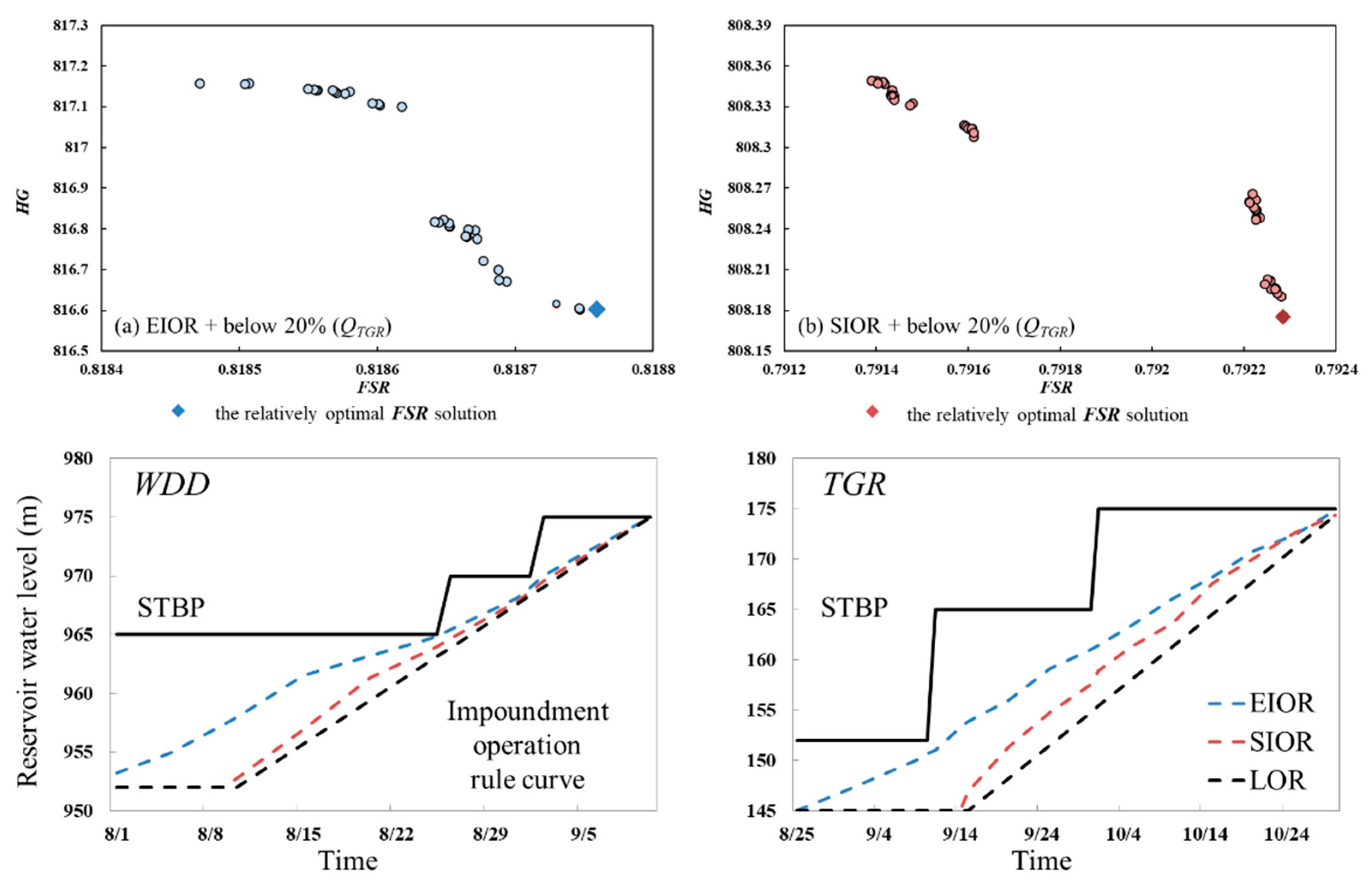
The above results demonstrate that GloFAS-Seasonal forecasts have the potential to give water managers the flexibility to employ early impoundment in the upper Yangtze River. Here, we try to analyze the EIOR and find its benefits. As an example, Figure 7 shows the Pareto-optimal solutions of EIOR (plot a) and SIOR (plot b) for the QTGR below the 20-percentile threshold. These Pareto-optimal solutions are averaged for derving parts of Table 4. We are employing three objective functions. Therefore, three subplots are needed for Pareto-optimal solutions to show three objectives in pairs. However, the flood control risk (R) of almost all Pareto-optimal solutions are equal to zero. Hence, we only show two objective functions (FSR and HG) in Figure 7. Each one of the 50 Pareto-optimal solutions obtained from the NSGA-II algorithm represents impoundment rule curve for each of the five cascade reservoirs. Figure 7 also shows EIOR and SIOR rule curves of WDD and TGR reservoirs focusing on the extreme solution of the FSR objective function. The figure shows that the average water level of EIOR is higher than SIOR for the selected 20-percentile threshold, while the risk of flooding is zero.
To illustrate the potential maximum benefits of EIOR, Figure 7 also shows a linear operation rule (LOR), which connects the initial water level to the top of STBP at the end of impoundment period. As a benchmark, LOR could present the maximum benefit of the EIOR from two parts where one is the earlier initial impoundment time and the other is the optimized rule curve. For curves of EIOR and LOR in Figure 7, Table 5 shows the benefit and risk of EIOR compared to the LOR. The proposed EIOR improves the FSR by 5.63% and increases HG by 4.02%. In conclusion, during dry years, our proposed methodology could significantly increase the hydropower generation and water utilization by employing GloFAS-Seasonal forecasts and early reservoir impoundment.
5. Conclusions
In this study, we evaluated the potential application of GloFAS-Seasonal forecasts for early reservoir impoundment in the upper Yangtze River. A cascade reservoirs impoundment simulation–optimization model was employed to select suitable low flow thresholds for decision-making for EIOR or SIOR. These thresholds were selected by analyzing the historical inflow data of WDD and TGR reservoirs, which were derived from Hua-Tan and Yi-Chang hydrologic stations. The performance of GloFAS-Seasonal reforecasts to predict the streamflow condition at these two hydrological stations was evaluated using AUC, ROCSS, and reliability diagram for two different lead times (LM1 and LM2) and selected thresholds. The main findings of our study can be summarized as follows:
(1) The low flow condition in September has a very significant impact on reservoir impoundment operation in the upper Yangtze River. The 20-percentile and 30-percentile selected thresholds of inflow at WDD and TGR are suitable for evaluating the possibility of early impoundment. These two selected thresholds can be used as a measure for flow condition and decision-making for early impoundment operation.
(2) All AUC values of reforecasts are greater than 0.6 which shows that GloFAS-Seasonal forecasts can be used to predict the streamflow condition according to the selected thresholds. However, AUC decreases from the LM1 (around 0.9) to the LM2 (below 0.8) as expected. The ROCSS reveals that both LM1 and LM2 are significantly better than climatology. The reliability diagrams also show that both LM1 and LM2 forecasts have more reliability and sharpness than climatology. Furthermore, results also indicate a tendency of the two lead time forecasts to over-estimate, which is more favorable for water managers.
(3) GloFAS-Seasonal forecasts with 2-month lead time (LM2) are valuable for reservoir impoundment operation. During dry years, the proposed EIOR improves the fullness storage rate by 5.63% and the annual average hydropower generation by 4.02% without increasing the risk of flooding.
This paper demonstrates that GloFAS-Seasonal forecasts has the potential to improve the standard impoundment operation rules in the upper Yangtze River and give water managers the flexibility to employ early impoundment.
Author Contributions
Conceptualization and software. K.C. and S.G.; Data Curation, J.W. and P.Q.; Formal Analysis, K.C., S.H. and S.S.; Writing—Original Draft Preparation, K.C. and M.R.N.; Writing—Review and Editing, S.G.
Funding
This study was funded by the National Key Research and Development Project (Grant NO. 2016YFC0402206) of China, the National Natural Science Foundation of China (Grant NO. 51879192), the “111 Project” Fund of China (B18037), the joint U.S.-China Clean Energy Research Center for Water-Energy Technologies (CERC-WET) project (2018YFE0196000) and the U.S. Department of Energy (DOE Prime Award # DE-IA0000018).
Acknowledgments
The authors would like to express their gratitude to anonymous reviewers for their insightful and constructive comments.
Conflicts of Interest
The authors declare no conflict of interest.
References
- Labadie, J.W. Optimal operation of multireservoir systems: State-of-the-art review. J. Water Res. Plan. Man. 2004, 130, 93–111. [Google Scholar] [CrossRef]
- Guo, S.L.; Zhang, H.G.; Chen, H.; Peng, D.Z.; Liu, P.; Pang, B. A reservoir flood forecasting and control system for China. Hydrolog. Sci. J. 2004, 49, 959–972. [Google Scholar] [CrossRef]
- Mehran, A.; Mazdiyasni, O.; AghaKouchak, A. A hybrid framework for assessing socioeconomic drought: Linking climate variability, local resilience, and demand. J. Geophys. Res. Atmos. 2015, 120, 7520–7533. [Google Scholar] [CrossRef]
- Rahnamay Naeini, M. A Framework for Optimization and Simulation of Reservoir Systems Using Advanced Optimization and Data Mining Tools. Ph.D. Dissertation, University of California Irvine, Irvine, CA, USA, 2019. [Google Scholar]
- Zhou, C.; Sun, N.; Chen, L.; Ding, Y.; Zhou, J.Z.; Zha, G.; Luo, G.L.; Dai, L.; Yang, X. Optimal Operation of Cascade Reservoirs for Flood Control of Multiple Areas Downstream: A Case Study in the Upper Yangtze River Basin. Water 2018, 10, 1250. [Google Scholar] [CrossRef]
- Wang, Q.S.; Zhou, J.Z.; Huang, K.D.; Dai, L.; Zha, G.; Chen, L.; Qin, H. Risk Assessment and Decision-Making Based on Mean-CVaR-Entropy for Flood Control Operation of Large Scale Reservoirs. Water 2019, 11, 649. [Google Scholar] [CrossRef]
- Zhou, Y.L.; Guo, S.L.; Xu, C.Y.; Liu, P.; Qin, H. Deriving joint optimal refill rules for cascade reservoirs with multi-objective evaluation. J. Hydrol. 2015, 524, 166–181. [Google Scholar] [CrossRef]
- Li, H.; Liu, P.; Guo, S.L.; Ming, B.; Cheng, L.; Zhou, Y.L. Hybrid Two-Stage Stochastic Methods Using Scenario-Based Forecasts for Reservoir Refill Operations. J. Water Res. Plan. Man. 2018, 144. [Google Scholar] [CrossRef]
- He, S.K.; Guo, S.L.; Chen, K.B.; Deng, L.L.; Liao, Z.; Xiong, F.; Yin, J.B. Optimal impoundment operation for cascade reservoirs coupling parallel dynamic programming with importance sampling and successive approximation. Adv. Water Resour. 2019, 131, 103375. [Google Scholar] [CrossRef]
- Batalla, R.J.; Gomez, C.M.; Kondolf, G.M. Reservoir-induced hydrological changes in the Ebro River basin (NE Spain). J. Hydrol. 2004, 290, 117–136. [Google Scholar] [CrossRef]
- Clark, E.J. Impounding reservoirs. J. Am. Water Works Assoc. 1956, 48, 349–354. [Google Scholar]
- Lund, J.R. Developing Seasonal and Long-Term Reservoir System Operation Plans Using HEC-PRM; Hydrologic Engineering Center: Davis, CA, USA, 1996. [Google Scholar]
- Lund, J.R.; Guzman, J. Derived operating rules for reservoirs in series or in parallel. J. Water Res. Plan. Man. 1999, 125, 143–153. [Google Scholar] [CrossRef]
- Liu, P.; Guo, S.L.; Xiong, L.H.; Li, W.; Zhang, H.G. Deriving reservoir refill operating rules by using the proposed DPNS model. Water Resour. Manag. 2006, 20, 337–357. [Google Scholar] [CrossRef]
- Liu, X.Y.; Guo, S.L.; Liu, P.; Chen, L.; Li, X.A. Deriving Optimal Refill Rules for Multi-Purpose Reservoir Operation. Water Resour. Manag. 2011, 25, 431–448. [Google Scholar] [CrossRef]
- Li, Y.; Guo, S.L.; Quo, J.L.; Wang, Y.; Li, T.Y.; Chen, J.H. Deriving the optimal refill rule for multi-purpose reservoir considering flood control risk. J. Hydro Environ. Res. 2014, 8, 248–259. [Google Scholar] [CrossRef]
- Wang, X.M.; Zhou, J.Z.; Ouyang, S.; Li, C.L. Research on Joint Impoundment Dispatching Model for Cascade Reservoir. Water Resour. Manag. 2014, 28, 5527–5542. [Google Scholar] [CrossRef]
- Zhou, Y.L.; Guo, S.L.; Chang, F.J.; Xu, C.Y. Boosting hydropower output of mega cascade reservoirs using an evolutionary algorithm with successive approximation. Appl. Energ. 2018, 228, 1726–1739. [Google Scholar] [CrossRef]
- Jasperse, J.; Ralph, M.; Anderson, M.; Brekke, L.D.; Dillabough, M.; Dettinger, M.D.; Haynes, A.; Hartman, R.; Jones, C.; Forbis, J. Preliminary Viability Assessment of Lake Mendocino Forecast Informed Reservoir Operations; Center For Western Weather and Water Extremes: San Diego, CA, USA, 2017. [Google Scholar]
- Liu, L.L.; Xiao, C.; Du, L.M.; Zhang, P.Q.; Wang, G.F. Extended-Range Runoff Forecasting Using a One-Way Coupled Climate-Hydrological Model: Case Studies of the Yiluo and Beijiang Rivers in China. Water 2019, 11, 1150. [Google Scholar] [CrossRef]
- Panagoulia, D. Impacts of Giss-Modeled Climate Changes on Catchment Hydrology. Hydrolog. Sci. J. 1992, 37, 141–163. [Google Scholar] [CrossRef]
- Yuan, X.; Wood, E.F.; Ma, Z.G. A review on climate-model-based seasonal hydrologic forecasting: Physical understanding and system development. Wires Water 2015, 2, 523–536. [Google Scholar] [CrossRef]
- Panagoulia, D.; Dimou, G. Sensitivity of flood events to global climate change. J. Hydrol. 1997, 191, 208–222. [Google Scholar] [CrossRef]
- Yuan, X.; Zhang, M.; Wang, L.Y.; Zhou, T. Understanding and seasonal forecasting of hydrological drought in the Anthropocene. Hydrol. Earth Syst. Sci. 2017, 21, 5477–5492. [Google Scholar] [CrossRef]
- Arnal, L.; Cloke, H.L.; Stephens, E.; Wetterhall, F.; Prudhomme, C.; Neumann, J.; Krzeminski, B.; Pappenberger, F. Skilful seasonal forecasts of streamflow over Europe? Hydrol. Earth Syst. Sci. 2018, 22, 2057–2072. [Google Scholar] [CrossRef]
- Bennett, J.C.; Wang, Q.J.; Robertson, D.E.; Schepen, A.; Li, M.; Michael, K. Assessment of an ensemble seasonal streamflow forecasting system for Australia. Hydrol. Earth Syst. Sci. 2017, 21, 6007–6030. [Google Scholar] [CrossRef]
- Demargne, J.; Wu, L.M.; Regonda, S.K.; Brown, J.D.; Lee, H.; He, M.X.; Seo, D.J.; Hartman, R.; Herr, H.D.; Fresch, M.; et al. The Science of NOAA’s Operational Hydrologic Ensemble Forecast Service. Bull. Am. Meteorol. Soc. 2014, 95, 79–98. [Google Scholar] [CrossRef]
- Block, P. Tailoring seasonal climate forecasts for hydropower operations. Hydrol. Earth Syst. Sci. 2011, 15, 1355–1368. [Google Scholar] [CrossRef]
- Delorit, J.; Ortuya, E.C.G.; Block, P. Evaluation of model-based seasonal streamflow and water allocation forecasts for the Elqui Valley, Chile. Hydrol. Earth Syst. Sci. 2017, 21, 4711–4725. [Google Scholar] [CrossRef]
- Baker, S.A.; Wood, A.W.; Rajagopalan, B. Developing Subseasonal to Seasonal Climate Forecast Products for Hydrology and Water Management. J. Am. Water Resour. Assoc. 2019, 55, 1024–1037. [Google Scholar] [CrossRef]
- Chen, K.B.; Guo, S.L.; He, S.K.; Xu, T.; Zhong, Y.X.; Sun, S.R. The Value of Hydrologic Information in Reservoir Outflow Decision-Making. Water 2018, 10, 1372. [Google Scholar] [CrossRef]
- Zhu, S.; Zhou, J.Z.; Ye, L.; Meng, C.Q. Streamflow estimation by support vector machine coupled with different methods of time series decomposition in the upper reaches of Yangtze River, China. Environ. Earth 2016, 75. [Google Scholar] [CrossRef]
- He, R.R.; Chen, Y.F.; Huang, Q.; Yu, S.N.; Hou, Y. Evaluation of ocean-atmospheric indices as predictors for summer streamflow of the Yangtze River based on ROC analysis. Stoch. Env. Res. Risk Assess. 2018, 32, 1903–1918. [Google Scholar] [CrossRef]
- Tan, Q.F.; Lei, X.H.; Wang, X.; Wang, H.; Wen, X.; Ji, Y.; Kang, A.Q. An adaptive middle and long-term runoff forecast model using EEMD-ANN hybrid approach. J. Hydrol. 2018, 567, 767–780. [Google Scholar] [CrossRef]
- Emerton, R.; Zsoter, E.; Arnal, L.; Cloke, H.L.; Muraro, D.; Prudhomme, C.; Stephens, E.M.; Salamon, P.; Pappenberger, F. Developing a global operational seasonal hydro-meteorological forecasting system: G1oFAS-Seasonal v1.0. Geosci. Model Dev. 2018, 11, 3327–3346. [Google Scholar] [CrossRef] [Green Version]
- Deb, K.; Pratap, A.; Agarwal, S.; Meyarivan, T. A fast and elitist multiobjective genetic algorithm: NSGA-II. IEEE Trans. Evolut. Comput. 2002, 6, 182–197. [Google Scholar] [CrossRef] [Green Version]
- Yeh, W.W.G. Reservoir Management and Operations Models - a State-of-the-Art Review. Water Resour. Res. 1985, 21, 1797–1818. [Google Scholar] [CrossRef]
- Lei, X.H.; Zhang, J.W.; Wang, H.; Wang, M.N.; Khu, S.T.; Li, Z.J.; Tan, Q.F. Deriving mixed reservoir operating rules for flood control based on weighted non-dominated sorting genetic algorithm II. J. Hydrol. 2018, 564, 967–983. [Google Scholar] [CrossRef]
- Celeste, A.B.; Billib, M. Evaluation of stochastic reservoir operation optimization models. Adv. Water Resour. 2009, 32, 1429–1443. [Google Scholar] [CrossRef]
- Zhao, T.T.G.; Zhao, J.S. Optimizing Operation of Water Supply Reservoir: The Role of Constraints. Math. Probl. Eng. 2014. [Google Scholar] [CrossRef]
- Naeini, M.R.; Yang, T.T.; Sadegh, M.; AghaKouchak, A.; Hsu, K.L.; Sorooshian, S.; Duan, Q.Y.; Lei, X.H. Shuffled Complex-Self Adaptive Hybrid EvoLution (SC-SAHEL) optimization framework. Environ. Modell. Softw. 2018, 104, 215–235. [Google Scholar] [CrossRef] [Green Version]
- Chang, L.C.; Chang, F.J. Multi-objective evolutionary algorithm for operating parallel reservoir system. J. Hydrol. 2009, 377, 12–20. [Google Scholar] [CrossRef]
- Tsai, W.P.; Chang, F.J.; Chang, L.C.; Herricks, E.E. AI techniques for optimizing multi-objective reservoir operation upon human and riverine ecosystem demands. J. Hydrol. 2015, 530, 634–644. [Google Scholar] [CrossRef]
- Uen, T.S.; Chang, F.J.; Zhou, Y.L.; Tsai, W.P. Exploring synergistic benefits of Water-Food-Energy Nexus through multi-objective reservoir optimization schemes. Sci. Total Environ. 2018, 633, 341–351. [Google Scholar] [CrossRef] [PubMed]
- Chen, Y.H.; Chang, F.J. Evolutionary artificial neural networks for hydrological systems forecasting. J. Hydrol. 2009, 367, 125–137. [Google Scholar] [CrossRef]
- Balsamo, G.; Pappenberger, F.; Dutra, E.; Viterbo, P.; van den Hurk, B. A revised land hydrology in the ECMWF model: A step towards daily water flux prediction in a fully-closed water cycle. Hydrol. Process. 2011, 25, 1046–1054. [Google Scholar] [CrossRef]
- Landman, W.A.; Beraki, A. Multi-model forecast skill for mid-summer rainfall over southern Africa. Int. J. Climatol. 2012, 32, 303–314. [Google Scholar] [CrossRef] [Green Version]
- Fundel, F.; Jorg-Hess, S.; Zappa, M. Monthly hydrometeorological ensemble prediction of streamflow droughts and corresponding drought indices. Hydrol. Earth Syst. Sci. 2013, 17, 395–407. [Google Scholar] [CrossRef] [Green Version]
- Manzanas, R.; Gutierrez, J.M.; Bhend, J.; Hemri, S.; Doblas-Reyes, F.J.; Torralba, V.; Penabad, E.; Brookshaw, A. Bias adjustment and ensemble recalibration methods for seasonal forecasting: A comprehensive intercomparison using the C3S dataset. Clim. Dynam. 2019, 53, 1287–1305. [Google Scholar] [CrossRef]
- Mason, S.J.; Graham, N.E. Conditional probabilities, relative operating characteristics, and relative operating levels. Weather Forecast. 1999, 14, 713–725. [Google Scholar] [CrossRef]
- Pappenberger, F.; Ramos, M.H.; Cloke, H.L.; Wetterhall, F.; Alfieri, L.; Bogner, K.; Mueller, A.; Salamon, P. How do I know if my forecasts are better? Using benchmarks in hydrological ensemble prediction. J. Hydrol. 2015, 522, 697–713. [Google Scholar] [CrossRef] [Green Version]
- Ogutu, G.E.O.; Franssen, W.H.P.; Supit, I.; Omondi, P.; Hutjes, R.W.A. Skill of ECMWF system-4 ensemble seasonal climate forecasts for East Africa. Int. J. Climatol. 2017, 37, 2734–2756. [Google Scholar] [CrossRef] [Green Version]
- Diez, E.; Orfila, B.; Frias, M.D.; Fernandez, J.; Cofino, A.S.; Gutierrez, J.M. Downscaling ECMWF seasonal precipitation forecasts in Europe using the RCA model. Tellus A 2011, 63, 757–762. [Google Scholar] [CrossRef]
- Jolliffe, I.T.; Stephenson, D.B. Forecast Verification: A Practitioner’s Guide in Atmospheric Science; John Wiley & Sons: Chichester, UK, 2012. [Google Scholar]
- Mason, S.J.; Stephenson, D.B. How do we know whether seasonal climate forecasts are any good? In Seasonal Climate: Forecasting and Managing Risk; Springer: Dordrecht, The Netherlands, 2008; pp. 259–289. [Google Scholar]
Figure 1.
Sketch map of the five cascade reservoirs in the upper Yangtze River.

Figure 2.
The flowchart of the parameterization–simulation–optimization (PSO) strategy to derive reservoir impoundment operation rule curves (a) input data of PSO, (b) optimization strategy of PSO, (c) concept of the seasonal top of buffer pool (STBP) and impoundment operation rules, similar to a previous study [9].

Figure 3.
The relationship between increased benefit ratio of EIOR and different flow groups of (a) QWDD and (b) QTGR.
Figure 3.
The relationship between increased benefit ratio of EIOR and different flow groups of (a) QWDD and (b) QTGR.

Figure 4.
The area under the ROC curve (AUC) values for GloFAS-Seasonal reforecast at Hua-Tan (left) and Yi-Chang (right) hydrologic stations.
Figure 4.
The area under the ROC curve (AUC) values for GloFAS-Seasonal reforecast at Hua-Tan (left) and Yi-Chang (right) hydrologic stations.

Figure 5.
Tercile plots and ROC skill score (ROCSS) for GloFAS-Seasonal reforecasts (a) 2-month lead at the Hua-Tan, (b) 1-month lead at the Hua-Tan, (c) 1-month lead at the Yi-Chang, and (d) 2-month lead at the Yi-Chang hydrologic station.
Figure 5.
Tercile plots and ROC skill score (ROCSS) for GloFAS-Seasonal reforecasts (a) 2-month lead at the Hua-Tan, (b) 1-month lead at the Hua-Tan, (c) 1-month lead at the Yi-Chang, and (d) 2-month lead at the Yi-Chang hydrologic station.

Figure 6.
Reliability diagrams of GloFAS-Seasonal reforecasts for comparing (a) two lead times and (b) thresholds.
Figure 6.
Reliability diagrams of GloFAS-Seasonal reforecasts for comparing (a) two lead times and (b) thresholds.

Figure 7.
Optimized EIOR and SIOR rule curves of WDD and TGR reservoirs focusing on fullness storage rate (FSR) for flow scenario group (below 20%) of QTGR.
Figure 7.
Optimized EIOR and SIOR rule curves of WDD and TGR reservoirs focusing on fullness storage rate (FSR) for flow scenario group (below 20%) of QTGR.


Table 1.
Characteristics of the five cascade reservoirs in the upper Yangtze River.
| Reservoir | Basin Area (Thousand km2) | Annual Top of Buffer Pool (m) | Top of Conservation Pool (m) | Total Storage Capacity (Billion m3) | Storage for Flood Control (Billion m3) | Installed Hydropower Capacity (GW) |
|---|---|---|---|---|---|---|
| WDD | 406.1 | 952 | 975 | 3.94 | 2.44 | 10.20 |
| BHT | 430.3 | 785 | 825 | 20.60 | 7.50 | 16.00 |
| XLD | 454.4 | 560 | 600 | 12.67 | 4.65 | 13.86 |
| XJB | 458.8 | 370 | 380 | 5.16 | 0.90 | 7.75 |
| TGR | 1000 | 145 | 175 | 45.07 | 22.15 | 22.50 |
Table 2.
Impounding periods of Standard impoundment operation rules (SIOR) and early impoundment operation rules (EIOR) for the five reservoirs.
Table 2.
Impounding periods of Standard impoundment operation rules (SIOR) and early impoundment operation rules (EIOR) for the five reservoirs.
| Reservoir | Initial Impoundment Time | Final Impoundment Time (SIOR, EIOR) | |
|---|---|---|---|
| (SIOR) | (EIOR) | ||
| WDD | Aug. 10th | Aug.1st | Sep. 10th |
| BHT | Aug. 10th | Aug.1st | Sep. 30th |
| XLD | Sep. 10st | Aug. 25th | Sep. 30th |
| XJB | Sep. 10st | Aug. 25th | Sep. 30th |
| TGR | Sep. 15th | Aug. 25th | Oct. 31st |
Table 3.
Seasonal top of buffer pool (STBP) for the five reservoirs in different periods.
| Reservoir | Seasonal Top of Buffer Pool (m) | |||||
|---|---|---|---|---|---|---|
| Aug.15th | Aug.25th | Sep.1st | Sep.10th | Sep.30th | Oct.31st | |
| WDD | 965 | 965 | 970 | 975 | 975 | 975 |
| BHT | 800 | 810 | 810 | 810 | 825 | 825 |
| XLD | 560 | 565 | 575 | 575 | 600 | 600 |
| XJB | 370 | 372 | 375 | 375 | 380 | 380 |
| TGR | 145 | 145 | 152 | 152 | 165 | 175 |
Table 4.
Benefit and risk results of the cascade reservoir system in response to the combination of historical flow group and impoundment rule.
Table 4.
Benefit and risk results of the cascade reservoir system in response to the combination of historical flow group and impoundment rule.
| Flow Group | EIOR | SIOR | |||||
|---|---|---|---|---|---|---|---|
| HG (108 kW·h) | FSR (%) | R (%) | HG (108 kW·h) | FSR (%) | R (%) | ||
| QWDD | below 20% | 813.784 | 82.68% | 0 | 805.070 | 79.78% | 0 |
| below 30% | 845.857 | 85.43% | 0 | 834.963 | 82.45% | 0 | |
| below 40% | 868.680 | 89.40% | 0 | 857.848 | 87.25% | 0 | |
| below 50% | 895.822 | 91.72% | 0 | 884.002 | 89.81% | 0 | |
| above 20% | 1025.617 | 99.25% | 1.802% | 1011.410 | 98.86% | 2.229% | |
| above 30% | 1040.072 | 99.98% | 2.035% | 1022.395 | 99.96% | 2.123% | |
| above 40% | 1060.128 | 100.00% | 2.924% | 1042.975 | 100.00% | 2.284% | |
| above 50% | 1074.293 | 100.00% | 3.730% | 1057.887 | 100.00% | 2.842% | |
| QTGR | below 20% | 816.973 | 81.86% | 0 | 808.284 | 79.18% | 0 |
| below 30% | 838.596 | 86.20% | 0 | 829.380 | 83.76% | 0 | |
| below 40% | 876.391 | 89.49% | 0 | 864.720 | 87.80% | 0 | |
| below 50% | 895.437 | 91.56% | 2.055% | 881.728 | 90.13% | 0 | |
| above 20% | 1024.592 | 99.23% | 2.217% | 1005.852 | 98.97% | 2.742% | |
| above 30% | 1042.250 | 99.70% | 2.313% | 1023.483 | 99.65% | 2.098% | |
| above 40% | 1048.775 | 99.88% | 2.237% | 1030.204 | 99.87% | 2.902% | |
| above 50% | 1072.242 | 99.96% | 2.263% | 1052.043 | 99.96% | 3.043% | |
Note: EIOR: early impoundment operation rules; SIOR: standard impoundment operation rules; HG: hydropower generation; FSR: fullness storage rate; R: flood control risk.
Table 5.
Comparison of the benefit and risk of EIOR and linear operation rule (LOR) rule curves for the QTGR below the 20-percentile threshold.
Table 5.
Comparison of the benefit and risk of EIOR and linear operation rule (LOR) rule curves for the QTGR below the 20-percentile threshold.
| Flow Group | Rule Curve in Figure 7 | Benefit and Risk | |||
|---|---|---|---|---|---|
| HG (108 kW·h) | FSR (%) | R (%) | |||
| QTGR | below 20% | LOR | 785.042 | 77.512% | 0 |
| EIOR | 816.601 | 81.876% | 0 | ||
| Increased ratio | 4.02% | 5.63% | 0 | ||
Note: QTGR: inflow to the Three Gorges Reservoir; LOR: linear operation rule; EIOR: early impoundment operation rules; HG: hydropower generation; FSR: fullness storage rate; R: flood control risk.
© 2019 by the authors. Licensee MDPI, Basel, Switzerland. This article is an open access article distributed under the terms and conditions of the Creative Commons Attribution (CC BY) license (http://creativecommons.org/licenses/by/4.0/).
Share and Cite
MDPI and ACS Style
Chen, K.; Guo, S.; Wang, J.; Qin, P.; He, S.; Sun, S.; Naeini, M.R. Evaluation of GloFAS-Seasonal Forecasts for Cascade Reservoir Impoundment Operation in the Upper Yangtze River. Water 2019, 11, 2539. https://doi.org/10.3390/w11122539
AMA Style
Chen K, Guo S, Wang J, Qin P, He S, Sun S, Naeini MR. Evaluation of GloFAS-Seasonal Forecasts for Cascade Reservoir Impoundment Operation in the Upper Yangtze River. Water. 2019; 11(12):2539. https://doi.org/10.3390/w11122539
Chicago/Turabian StyleChen, Kebing, Shenglian Guo, Jun Wang, Pengcheng Qin, Shaokun He, Sirui Sun, and Matin Rahnamay Naeini. 2019. "Evaluation of GloFAS-Seasonal Forecasts for Cascade Reservoir Impoundment Operation in the Upper Yangtze River" Water 11, no. 12: 2539. https://doi.org/10.3390/w11122539
Note that from the first issue of 2016, this journal uses article numbers instead of page numbers. See further details here.