Article

Potential of A Trait-Based Approach in the Characterization of An N-Contaminated Alluvial Aquifer

by
Tiziana Di Lorenzo
1,*,
Alessandro Murolo
2,
Barbara Fiasca
2,
Agostina Tabilio Di Camillo
2,
Mattia Di Cicco
2 and
Diana Maria Paola Galassi
2
1
Research Institute on Terrestrial Ecosystems (IRET-CNR), Via Madonna del Piano 10, 50019 Sesto Fiorentino, Firenze, Italy
2
Department of Life, Health and Environmental Sciences, University of L’Aquila, Via Vetoio 1, Coppito, 67100 L’Aquila, Italy
*
Author to whom correspondence should be addressed.
Water 2019, 11(12), 2553; https://doi.org/10.3390/w11122553
Submission received: 25 October 2019 / Revised: 19 November 2019 / Accepted: 28 November 2019 / Published: 3 December 2019

Abstract

:
Groundwater communities residing in contaminated aquifers have been investigated mainly through taxonomy-based approaches (i.e., analyzing taxonomic richness and abundances) while ecological traits have been rarely considered. The aim of this study was to assess whether a trait analysis adds value to the traditional taxonomy-based biomonitoring in N-contaminated aquifers. To this end, we monitored 40 bores in the Vomano alluvial aquifer (VO_GWB, Italy) for two years. The aquifer is a nitrate vulnerable zone according to the Water Framework Directive. The traditional taxonomy-based approach revealed an unexpectedly high biodiversity (38 taxa and 5725 individuals), dominated by crustaceans, comparable to that of other unpolluted alluvial aquifers worldwide. This result is in contrast with previous studies and calls into question the sensitivity of stygobiotic species to N-compounds. The trait analysis provided an added value to the study, unveiling signs of impairments of the groundwater community such as low juveniles-to-adults and males-to-females ratios and a crossover of biomasses and abundances curves suggestive of an intermediate alteration of the copepod assemblages.

1. Introduction

The taxonomy-based approach, which is traditionally focused on the analysis of taxonomic richness and abundances, has long been used to characterize and assess the impairment of freshwater ecosystems [1]. Following this approach, biological samples are collected from impaired sites and the taxa are identified, enumerated, and then compared to those of pristine reference sites (e.g., [2]). Trait-based approaches have been developed over the years alternatively to the taxonomy-based one or, more often, in combination with it. Traits are measurable physiological, morphological, and ecological characteristics of organisms, populations, or communities, such as the body size, the trophic role, the duration of life cycle, the reproductive rate, and so forth [3]. The trait-based approach allows understanding ecosystems in ways often unattainable by studies that are exclusively focused on taxonomic diversity. In the first place, traits i) reflect the species (population or community) adaptation level to their environment [4] and ii) can be used as measures of functional diversity [5]. Secondly, trait-based approaches work well across geographies since many traits are shared by widely distributed taxa [3]. From this perspective, some traits can be even applied across ecoregions [6]. Other strengths are that they add diagnostic knowledge, do not require new sampling methodology, and can supplement taxonomic analyses, while weaknesses are redundancy, autocorrelation, and difficulty in the measurements [3]. One of the most useful and fascinating aspects of trait-based approaches is that they can reveal a substantive trait variation (e.g., metabolic changes) before the taxonomic composition of the community is impaired by the loss of some species [1]. Similarly, some traits may have an earlier diagnostic potential regarding ecosystem recovery [1]. However, the decision to prefer a trait-based approach over a taxonomy-based one must be taken with caution; rather, the best option is the combination of the two approaches, at least for freshwater ecosystems [1]. In fact, trait-based approaches may fail to diagnose impacts on imperiled species which are rare in terms of abundance, because of functional redundancy [1]. On the other hand, the diagnostic power of a taxonomy-based approach decreases if the community is not characterized at the species level, but rather described at the genus or even family resolution, as required in several biomonitoring programs [7,8].
Although trait-based approaches have an old tradition in freshwater ecology (reviewed in [1]), they have not been widely applied to groundwater ecosystems. Groundwater habitats, and alluvial aquifers in particular, are characterized by lack of light and by environmental conditions that are more stable compared to surface water environments [9]. The absence of light precludes primary production by photosynthesis, so groundwater ecosystems are generally reliant on allochthonous organic carbon from surface environments [10,11]. However, particulate organic matter is not always available to groundwater food webs because it is intercepted in the soil and the unsaturated zone [10]. Consequently, the basal food source for stygofauna (obligate groundwater-dweller fauna) consists mainly of bacteria and the organic matter that is assimilated by microorganisms [12,13,14]. Unlike surface waters, groundwater ecosystems support only a few vertebrate species and the invertebrate assemblages are generally dominated by crustaceans [15,16]. Groundwater invertebrate assemblages also may include mites, oligochaetes and, rarely, insects and mollusks [9,17]. Copepods, amphipods, isopods, and syncarids are crustacean taxa commonly collected in healthy groundwater ecosystems [18,19]. The response of stygobiotic communities to impairments due to anthropic pressures has often been examined through taxonomy-based approaches [20,21,22,23]. Recently, some stygofaunal traits have proven to be useful in assessing the response of groundwater communities to groundwater flooding [24], carbon input [25,26], habitat structure [27,28] and chemical contamination [20,29,30,31]. However, the selection of a set of traits that best characterize groundwater communities is still to come.
Alluvial aquifers are particularly prone to organic pollution as their outcrops are frequently cultivated or occupied by urban settlements [21,32]. As a result, an increase in the concentrations of nitrate, nitrite, and ammonium is often observed in groundwater, with long-lasting exceedances of the legal limits [22]. Organic contamination is known to cause a change in the structure and composition of stygobiotic assemblages. Elevated concentrations of N-compounds, due to contamination through sewage and septic tank leaks, or due to the overuse of natural and synthetic fertilizers, alter the structure of groundwater communities through favoring the proliferation of surface water organisms [22,33,34]. However, the ecological studies conducted on alluvial aquifers contaminated by N-compounds are still rather scarce and reliant on the taxonomy-based approach [21,35].
The aim of this study was to evaluate the performance of a trait-based approach in the ecological characterization of an alluvial aquifer with a ten-year history of N-compound contamination. To this end, we analyzed the biological assemblages of the Vomano alluvial aquifer (central Italy) that, in 2010, was designated as a Nitrate Vulnerable Zone (NVZ) under the Water Framework Directive (EC, 2000) due to a nitrate contamination affecting over 50% of the groundwater body volume [36]. We measured five ecological traits and compared the results with those deriving from the traditional approach based on taxonomic richness and abundance distribution.

2. Materials and Methods
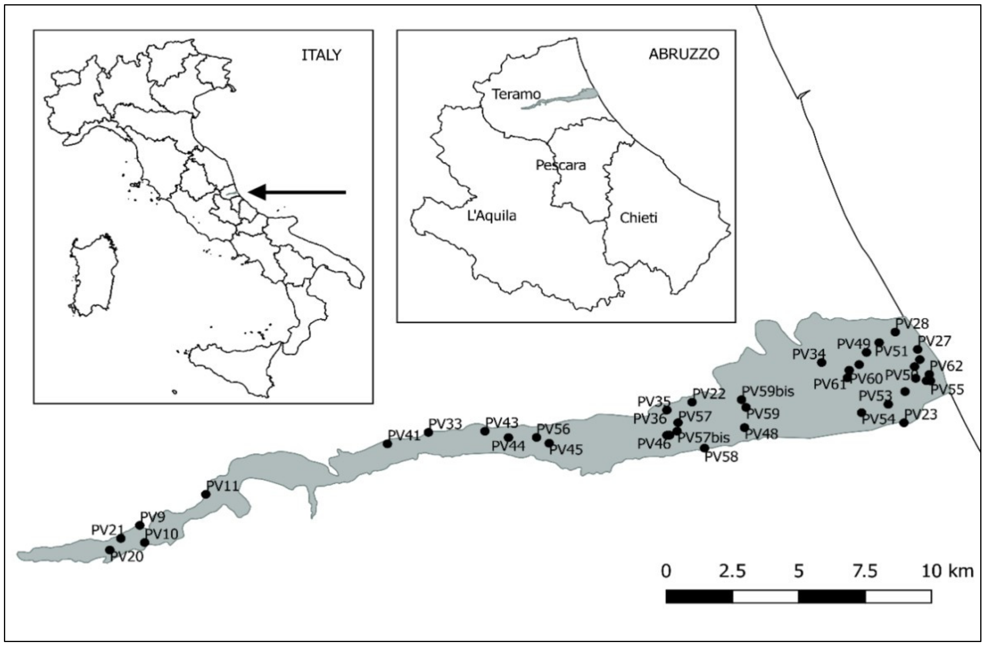
2.1. Study Area

The study was performed on an alluvial aquifer (VO_GWB; Figure 1) located in the hydrographic basin of the River Vomano (Italy). The outcrop of the aquifer is 30 km2. VO_GWB is mainly fed by the River Vomano waters and rainfalls which reach the base of the aquifer in a few weeks [36,37]. The alluvial deposits of VO_GWB consist mainly of gravel and sand interbedded by silty-clay lenses of limited extension [37]. The basement of the aquifer (at a depth of about 35 m) is made up of silty-clay deposits of very low permeability [37]. The groundwater flow is NW–SE directed, and the aquifer mean discharge is 1.3 × 10⁻² m3/s [36]. VO_GWB is used for drinking and industrial and agricultural purposes. The chemical and quantitative status of VO_GWB is routinely monitored by the local environmental authority according to the requirements of the Water Framework Directive [38] and Groundwater Daughter Directive [39]. In 2010, VO_GWB was designated as a Nitrate Vulnerable Zone (NVZ) under the Water Framework Directive [38] due to a persisting (>10 years) nitrate contamination [36].
Groundwater sampling occurred in 40 bores used for agricultural purposes (Figure 1). Groundwater organisms and water samples for chemical analyses were collected from shallow bores (up to 30 m deep) in autumn 2014 and spring and winter 2015 for a total of 97 samples. The altitude of the bores varied from 0 to 240 m above sea level and the depth from 2 to 30 m below the soil level. The piezometric level, measured using a freatimeter (PASI, Turin), was in the range 0.5–25.9 m below ground level. The bores’ distance from the River Vomano varied from a minimum of 167 m to a maximum of 1733 m.
Groundwater flow of VO_GWB is considered basal, meaning that the groundwater undergoes remixing at all aquifer depths [37]. Preliminary investigations in which the aquifer volume was arbitrarily subdivided into three (0–10 m, 11–20 m, and 21–30 m deep) or two (0–15 m, 16–30 m deep) sectors did not reveal any significant environmental or biological pattern (Supplementary Materials: PRELIMINARY). For this reason, the aquifer was investigated as a unique groundwater unit.

2.2. Biological Survey

Bores were sampled with either an immersion pump (IP), a manual pump (MP), or a modified Cvetkov net [40], depending on the bore type (drilled or hand-dug). Five hundred liters of groundwater were withdrawn using IP and 50 L using MP. The volumes were subsequently filtered by a 60 μm mesh net to collect groundwater fauna. The modified Cvetkov net, equipped with a weight anchored to the tail, was lowered into the hand-dug bores to the bottom and subsequently hauled to filter the entire column of bore water. Ten hauls were performed in each bore [41]. The collected samples were transported in 1 L plastic vials to the laboratory within 6 h and then fixed in 70% ethanol solution. In the laboratory, specimens were sorted under a stereomicroscope at 16× magnification and identified to the lowest taxonomic level possible. Copepods were identified to species level after dissection and subsequent observation with a Leica DM 2500 optical microscope, following dichotomous keys [42,43] and more recent taxonomic papers.
Depending on the degree of adaptation to groundwater, each taxon was classified either as stygobiont (SB: species strictly associated to groundwater habitats, where it completes the whole life cycle; [44]) or non-stygobiont (nSB: epigean species accidentally or occasionally occurring in groundwater). Each specimen of the dominant taxon (Copepoda; see par. 4.) was individually photographed under a Leica M205C stereomicroscope. Length and width were measured with the software LAS (Leica Application Suite, Version 4.7.1 of Leica Microsystems, Wetzlar, Germany). Copepod lengths (in mm) were measured from the tip of the cephalic shield to the end of caudal rami, while width (in mm) was measured at the larger somite bearing legs. Sex was identified in adult individuals. Afterwards, copepod body dimensions (length and width) were converted to species–specific biovolume (in nL) using Equation (1) [45]:
BV = a × b 2 × C F
where BV = biovolume, a = length (mm), b = width (mm), and CF is a correction factor that accounts for the body shape. CF varied from 230 to 750 according to the body shape outlines of each specimen [46]. The biovolumes were then converted into individual fresh weights assuming a specific gravity of 1.1 [24]. The dry mass (mg) was estimated assuming a dry/wet weight ratio of 0.25 and the dry weight carbon content (biomass) was assumed to be 40% of the dry mass [47].

2.3. Environmental Survey

Physicochemical parameters, such as electrical conductivity (µS/cm), pH, dissolved oxygen (mg/L), and temperature (°C), were measured in situ with a multiparametric probe (WTW 3430 SET G). Two liters of groundwater were collected and stored in high-density polyethylene bottles for further chemical analyses aimed at measuring the concentrations of the 110 chemical compounds indicated in the Supplementary Materials (ENV). Particulate organic matter (POM) was obtained as the difference between the sediment weight deprived of the faunal component and dehydrated at 105 °C and that obtained after combustion of the organic fraction at 540 °C.

2.4. Data Analysis: Environmental Variables

As subsequent samples from the same bore must be considered temporal pseudoreplicates producing bias in the statistics [48], the mean values of each abiotic variable were used in the statistical analyses in the place of the raw data. Only 22 variables out of 110 were analyzed, that is, only those showing a standard deviation (SD) ≠ 0 (Table 1) so as to exclude irrelevant variables in the statistical models. Potential environmental patterns were investigated through a principal component analysis (PCA) on the basis of the Euclidean distance matrix. Prior to PCA, data were normalized and a Draftsman’s plot was used to examine the correlation among the environmental variables [49,50].

2.5. Taxonomy-Based Approach

The exhaustiveness of the biological sampling effort was assessed through taxonomic richness estimations, using nonparametric estimators, namely, Chao1, Chao2, Jackknife1 and Jackknife2, Bootstrap, Michaelis-Menton (MM), and Ugland-Gray-Ellingsen (UGE) [51]. Values were estimated by means of 999 randomizations without replacement.
Abundances were expressed as ind/L dividing the number of individuals of each sample by its volume (liters). Raw data are available in the Supplementary Materials (BIO_VOGWB). Abundances of temporal replicates were summed per each sampling site prior to being used in the statistical analyses. Potential biological patterns were examined using a non-metric multidimensional scaling (nMDS) analysis, incorporating Bray-Curtis similarities after adding a dummy variable equal to 1 [49]. Prior to nMDS, data were log(x + 1)-transformed to approximately conform the data to normality. BIO-ENV analyses [52], based on Spearman’s rank correlations, were performed to find the ‘best’ match between the biological and the environmental data. The statistical significance of the results of the BIO-ENV routine was tested by the global BIO-ENV match permutation test whereby each set of samples was randomly permuted 99 times relative to the others [52]. In addition to multivariate analyses, univariate statistics was performed to assess correlation between individual environmental variables and cumulative abundances per sampling site. The significance was assessed through a permutation test performed by randomly shuffling 999 times the independent variable (i.e., the environmental variables). The permutation test was selected because it is more powerful than tests based on normal theory assumptions when data distribution departs substantially from normality, as it was the case for the data of this study. Regressions were performed with the ape library in R 3.0.2 [53].
Finally, the structure of the biological assemblages of N-compound-contaminated alluvial aquifers other than VO_GWB was obtained from literature by using i) ISI Web of Knowledge SM (© 2010 Thomson Reuters, Toronto, ON, CA) with the following strings applied to the topic field: “aquifer” and “stygo*” and “nitrate” or “nitrite” or “ammon*”; ii) Google with the same setting as for i).

2.6. Trait-Based Approach

Potential biological patterns were examined using the following traits and the statistical settings as for the taxonomy-based approach (par. 2.5): Trait#1 (crustaceans vs. non-crustaceans); Trait#2 (SB vs. nSB); Trait#3 (adults vs. juveniles); Trait#4 (males vs. females); Trait#5 (biomass). Since copepod crustaceans accounted for 98% of the aquifer biodiversity, Traits#2–5 were analyzed with respect to copepods only. We analyzed these traits since previous studies have demonstrated that they are reliable indicators of impairment of groundwater communities, with particular references to organic contamination. In detail: i) groundwater assemblages dominated by non-crustacean taxa and a high nSB/SB ratio should be considered impaired [34]; ii) the sex ratio of some populations of copepods may be skewed in favor of female individuals in impaired water bodies [54,55,56]; iii) the development of juvenile copepods is slowed down in populations exposed to ammonium with respect to control populations [57]; and the survival of copepodids under N-compound exposure is significantly lower than that of adult individuals of the same species [58]. Finally, we analyzed the biomass because its relationship with abundances provides key information about community impairment [49,50]. Distributions of copepod species abundances and biomasses were compared on the same terms with k-dominance curves, namely applying the Abundance/Biomass Comparison method (ABC) with the following assumptions [52]: i) in an undisturbed community, the k-dominance curve for biomass lies above the curve of abundances for its entire length; ii) as impairment occurs and becomes more severe, the abundance curve lies above the biomass curve, in part, or completely. The W statistic was used to algebraically interpret the position of the curves, the metric values being in the range −1,1 (though neither limit is likely to be attained), with W close to 1 indicating undisturbed condition, W close to 0 indicating intermediate impairment, and W close to −1 indicating severe impairment [52].
Eventual significant patterns of each trait were explored by nMDS plots performed on the Bray–Curtis dissimilarity matrices as in the taxonomy-based approach (par. 2.5). Similarly, BIO-ENV analyses [52] and permutational regressions were used to explore the correlations between the environmental variables and the data of the individual traits.

3. Results

3.1. Environmental Variables

Mean and SD values of the 22 variables with SD ≠ 0 are shown in Table 1.
Mean values of nitrites and nitrates were indicative of contamination according to the legal threshold values (respectively: 0.05 and 50 mg/L) set by Italian regulation [59].
Nitrite contamination was detected in 24 out of 40 bores, 20 of which also showed a nitrate contamination. Overall, bores contaminated by nitrates were 30 out of 40. Fifteen out of 40 bores were contaminated by ionized ammonium. Seven of these bores were also contaminated by nitrates while nine were contaminated by nitrites. Overall, contamination by N-compounds (nitrites, nitrates, and ionized ammonium) involved 36 bores out of 40. The PCA (matrix: 22 variables × 40 sampling sites; plot not shown) explained only 34% of the cumulative variance of the environmental data on the first two axes, failing to highlight a clear pattern of the environmental variables. This result implies that the chemical and physicochemical conditions of VO_GWB were uniform through the aquifer and there were no areas with environmental peculiarities.

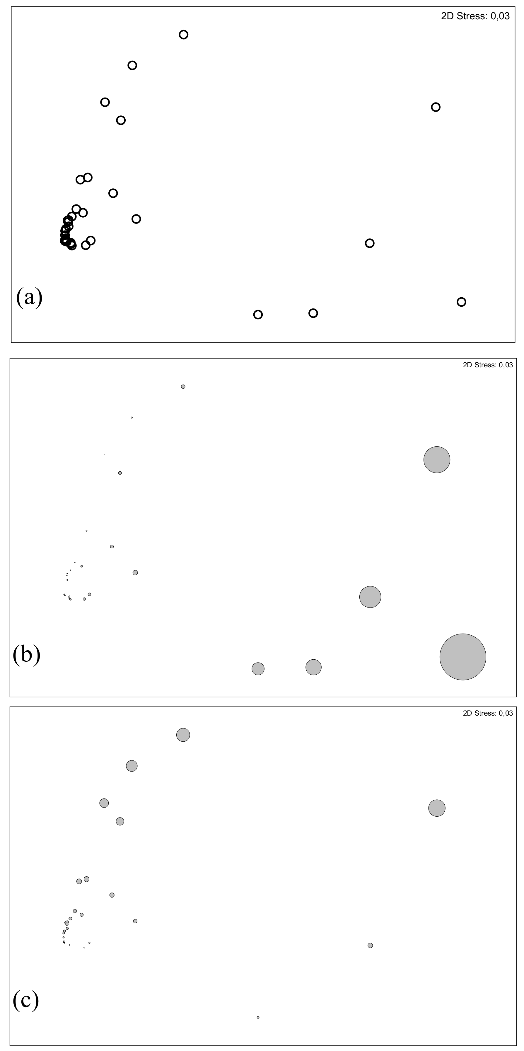
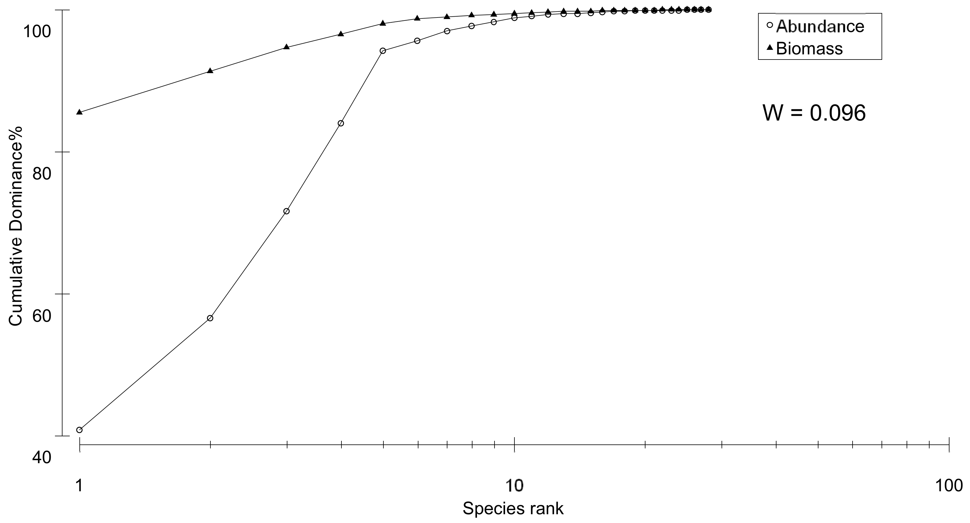
3.2. Taxonomy-Based Approach

The stygofauna collected in VO_GWB accounted for 5724 individuals belonging to 38 taxa (35 crustaceans, 2 insect instars, and 1 water mite). Crustaceans were dominant in terms of abundances (99.70%), followed by insects (0.23%) and water mites (0.07%). Among crustaceans, the taxon Copepoda accounted for 97.93% of the total abundances, Amphipoda for 1.52%, Isopoda for 0.02%, Syncarida for 0.16%, and Ostracoda for 0.37%. Two out of seven non-parametric estimators reached the asymptotes, indicating the exhaustiveness of the sampling effort (Supplementary Materials: SRC). The remaining estimators indicated that the sampling effort was such to cover from 67% (Chao1) to 90% (Bootstrap) of the expected biodiversity of the aquifer.
Literature data related to N-compound concentrations and groundwater taxonomic richness in 11 alluvial aquifers worldwide are reported in Table 2.
The stygobiotic cyclopoid Diacyclops cosanus (Dco) occurred in 15 bores out 40 and was the species with the widest distribution in VO_GWB. The remaining 35 taxa occurred in less than 12 bores out of 40 and 24 taxa (12 of which were stygobiotic) occurred in less than 4 bores. Bore PV28 (13 m deep) showed the highest biodiversity, with 11 taxa, 7 of which were stygobiotic, followed by PV48 (20 m deep) with 10 taxa, 9 of which were stygobiotic. More than 50% of the bores (namely, 23 out of 40) were characterized by a maximum of three taxa and no taxa were collected from three bores, namely, from P26 (18 m deep), PV53 (10 m deep), and PV62 (8 m deep).
The nMDS plot (Figure 2; 2D stress: 0.03; matrix: 38 variables × 40 sampling sites) showed a group of 27 bores of different depths (from 4 to 30 m deep), almost completely overlapping at the center of the plot and surrounded by 11 bores (from 2 to 25 m deep) located at different distances. Thirteen out of 38 taxa were exclusive of the bores overlapping in the center of the plot, namely, the copepods Paracyclops fimbriatus (Pfi), Bryocamptus pygmaeus (Bpy), Eucyclops serrulatus (Ese), Diacyclops maggii (Dma), Graeteriella unisetigera (Gun), Nitokra hibernica (Nhi), Nitocrella fedelitae (Nfi), Nitocrella achaiae (Nac), Bryocamptus dentatus (Bde), Elaphoidella plutonis (Epl), Pseudectinosoma reductum (Pre), the amphipod Niphargus sp. 2 (Nsp2), and a species belonging to the Coleoptera Elmidae (Elm). Three species, namely, the copepods Diacyclops bicuspidatus (Dbic) and Nitocrella kunzi (Nku), and the amphipod Niphargus sodalis (Nso), occurred exclusively in the not-overlapping bores (Figure 2 and Supplementary Materials: BIO_VOGWB).
The BIO-ENV analysis showed that there was no significant explanatory relationship between the environmental variables and the matrix of the 38 taxa collected in VO_GWB. In fact, the sole environmental variable which best correlated to the taxa abundances was POM (ρ = 0.436) and the best n-dimensional combination consisted of five variables, namely, electrical conductivity, pH, nitrites, nitrates, and ionized ammonium. However, the real value of ρ fell within the 95% confidence limit of the normal distribution of randomly permuted values of ρ (p-value = 14%), indicating that the null hypothesis of no relationship between the best subset of environmental variables and the community structure should not be rejected. Univariate analyses gave significant results. In fact, cumulative densities were negatively correlated, although weakly, to electrical conductivity, dissolved oxygen, nitrates, sulphates, calcium, and sodium (Supplementary Materials: REGR). However, R2 values were <20% for all parameters except for electrical conductivity (R2 = 57%), meaning that the regression models had a low predictive potential.

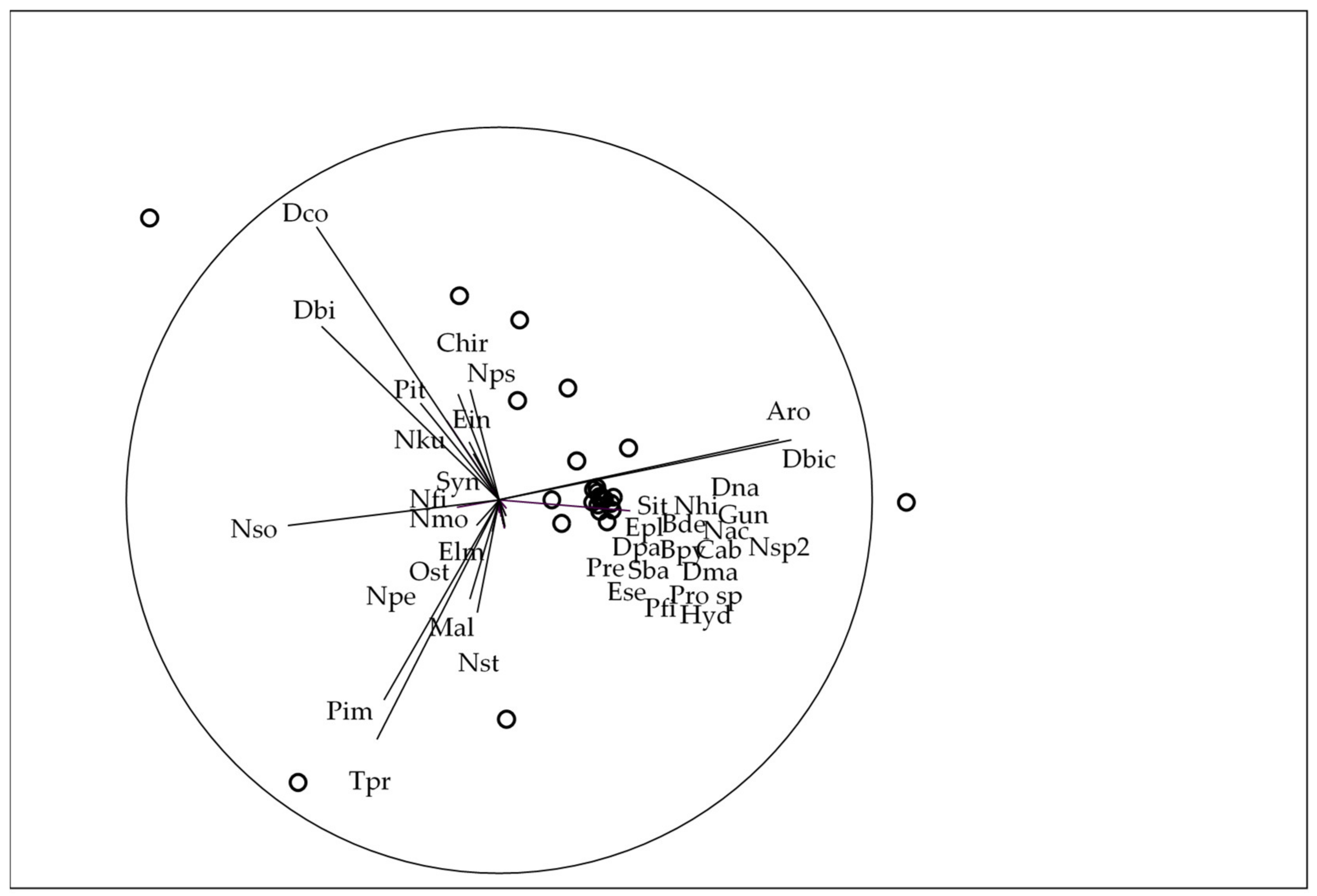
3.3. Trait-Based Approach

Trait#1 (crustacean vs. non-crustacean taxa). VO_GWB was dominated by crustaceans, occurring with 35 out of 38 taxa. The nMDS returned an arched, or horseshoe, pattern. This effect is very common in datasets in which there is a progressive turnover of a dominant variable [67]. In fact, the nMDS bubble plot showed that the arch effect was due to the turnover of crustacean taxa (Supplementary Materials: nMDS_T1). The BIO-ENV analysis indicated no significant relationship between the best subsets of environmental variables (POM: ρ = 0.435; p-value = 18%) and the abundances of crustacean and non-crustacean taxa. Univariate analyses did not highlight significant correlation between the cumulative abundances of crustaceans (or non-crustaceans) and the individual environmental variables.
Trait#2 (SB vs. nSB taxa). Seventeen out of 38 taxa were nSB and 21 were SB (Supplementary Materials: BIO_VOGWB). The nMDS (2D Stress: 0.03) showed that SB and nSB taxa occurred almost in all bores (Figure 3a), however, with different abundances.
SB abundances (Figure 3b) were higher in the eight bores located in the upper sector of the plot while nSB abundances (Figure 3c) were higher in the lower sector of the plot, and in particular, in five bores. The group of eight bores with the highest abundances of SB taxa differed from the group of the five bores in the mean values of some environmental variables. Specifically, the average values of POM (0.44 mg/L), nitrite (9 mg/L), and ionized ammonium (0.031 mg/L) were lower in the bores with high densities of SB than in those with high densities of nSB (POM: 1.33 mg/L, nitrite: 13 mg/L, ionized ammonium: 0.644 mg/L). On the other hand, the mean values of electrical conductivity (1237 μS/cm), nitrates (79 mg/L), sulphates (109 mg/L), chloride (51 mg/L), calcium (156 mg/L), and sodium (53 mg/L) were higher in the sites with high densities of SB than in those with high densities of nSB (electrical conductivity: 835 μS/cm, nitrates: 43 mg/L, sulphate: 45 mg/L, chloride: 30 mg/L, calcium: 105 mg/L, and sodium: 31 mg/L). However, the BIO-ENV analysis indicated no significant relationship between the best subsets of environmental variables (POM: ρ = 0.443; p-value = 16%) and the densities of the two ecological categories. The univariate analyses highlighted a significant negative correlation between SB copepod abundances and bore depth (Supplementary Materials: REGR), however, with an R2 equal to 11%. The abundances of nSB copepods were negatively correlated to electrical conductivity, dissolved oxygen, nitrate, sulphates, calcium, and sodium (Supplementary Materials: REGR). R2 values were <20% for all parameters except for electrical conductivity (R2 = 57%).
Trait#3 (adults vs. juveniles). All copepod species were collected with adults and juveniles with a few exceptions, such as the nSB species Nitokra hibernica and the SB species Nitocrella fedelitae, Nitocrella morettii, Nitocrella kunzi, Bryocamptus dentatus, and Pseudectinosoma reductum, which were collected with adults only. The nMDS plot (Supplementary Materials: nMDS_T3) showed no clear separation of the bores, however, the bubble plot highlighted that adult copepods were slightly more numerous than juveniles almost in every bore. The univariate analyses highlighted a significant negative correlation between adult copepod abundances and electrical conductivity, dissolved oxygen, nitrate, sulphates, calcium, and sodium (Supplementary Materials: REGR). A significant negative correlation was assessed between juvenile abundances and electrical conductivity, sulphates, calcium, and sodium as well (Supplementary Materials: REGR). However, R2 values were all <20%, except for electrical conductivity (R2 > 50%).
Trait#4 (males vs. females). Twelve copepod species occurred with more females than males, nine species with more males than females, and seven species with the same number of males and females. Overall, the average abundance ± SD of males was 0.26 ± 0.70 ind/L and that of females was 0.67 ± 2.13 ind/L, with a sex ratio equal to 0.38. The nMDS did not show a clear pattern (Supplementary Materials: nMDS_T4). The BIO-ENV analysis indicated no relationship between the best subsets of environmental variables (POM: ρ = 0.437; p-value = 18%) and the abundances of males and females. The univariate analyses highlighted a significant negative correlation between male abundances and electrical conductivity, dissolved oxygen, nitrate, sulphates, and calcium (Supplementary Materials: REGR). A significant correlation was assessed between female abundances and electrical conductivity, dissolved oxygen, nitrates, sulphates, calcium, and sodium as well (Supplementary Materials: REGR). However, R2 values were <20% for all parameters and for both males and females, except for electrical conductivity (R2 > 43%).
Trait#5 (biomass). The total dry weight carbon (mean ± SD) was 0.012 ± 0.061 mg/L C. Multivariate analyses did not reveal significant patterns. The univariate analyses highlighted a significant negative correlation between biomass and electrical conductivity, dissolved oxygen, and calcium (Supplementary Materials: REGR). However, R2 values were all <20%, except for electrical conductivity (R2 = 42%). The biomass and abundance curves partially crossed at about the 20th species but since both curves were close to 100% at this point, the crossover was unclear (Figure 4). However, the W metric equal to 0.096 was indicative of a moderate impairment of the copepod assemblages.

4. Discussion

The taxonomic richness of VO_GWB was high and consistent with previous studies in other European and non-European alluvial aquifers [60,64,66,68,69], both at the local and the regional scales [15,70]. However, the number of species collected in VO_GWB is surprisingly high if considering the persisting N-compound contamination which occurred in 90% of the aquifer. This study highlighted the high taxonomic richness and abundances of the assemblages of VO_GWB with respect to those of other alluvial aquifers worldwide contaminated by N-compounds. The taxonomic richness (38 taxa) and the abundances (5725 individuals) of VO_GWB were comparable to those of pristine alluvial aquifers. Such a result is in contrast with previous data showing that freshwater invertebrates are highly sensitive to N-compounds [71]. From this point of view, the results of this study represent a novelty and require further ecotoxicological investigations. In fact, to date, ecotoxicological studies with N-compounds have been focused mainly on non-stygobiotic invertebrates, with the exception of the study carried out by [58], who analyzed the sensitivity of the stygobiotic cyclopoid Diacyclops belgicus (not found in VO_GWB) to ionized ammonium. The low number of ecotoxicological data concerning stygobiotic species, and the reasons behind the difficulty in carrying out such studies, have recently been reviewed by [72], who have also claimed as unrealistic the probability of gathering new data in the near future. Thus, the high taxonomic richness and abundances observed in VO_GWB will likely remain unsupported by ecotoxicological considerations for some more time.
The traditional taxonomy-based approach showed that most taxa were collected only in a few bores and showed, therefore, restricted distributions as already observed in other studies (e.g., [64,66]). The most widespread species in VO_GWB, D. cosanus, is known to be highly tolerant to elevated values of salinity and electrical conductivity, being collected in other N-contaminated alluvial aquifers, in brackish coastal groundwater in southern Italy, and in sulfidic saturated karst [21]. The occurrence of epigean species in the deeper sectors of VO_GWB is recurrent in alluvial aquifers, especially in those polluted by contaminants of organic origin (e.g., [22,64]). The weak correlations of the environmental and biological variables are a common result in groundwater studies, in particular, in aquifers that are highly homogeneous from a physicochemical point of view [22,66,73]. In this study, the variance explained by the univariate models was low and this indicated that further factors, in addition to those already investigated, must be taken into account in the future to better explain the observed biological patterns. For instance, copepod species interactions could play a role in determining the biological assemblages in VO_GWB as already observed in other aquifers [74]. Similarly, previous studies showed that the grain size composition of sediments [75,76,77], and the lowering of the groundwater table [21,75], could influence the biological assemblage’s patterns in alluvial aquifers.
Trait#1 (crustaceans vs. non-crustaceans) highlighted the predominance of crustaceans in VO_GWB. This result is in contrast with previous studies [21,33,62] which showed that crustacean abundances are lower than those of non-crustaceans in aquifers polluted by N-enriched infiltration waters.
Trait#2 provided additional information to this study, highlighting that stygobiotic species seemed to thrive in the bores where non-stygobiotic species were less abundant. The environmental variables did not entirely explain such a pattern. Hence, additional factors should be investigated such as the isolation of the bores from the surface. In fact, groundwater habitats characterized by intense water exchanges with the surface environment often exhibit a predominance of generalist non-stygobiotic fauna, while isolated groundwater sites show a predominance, or even an exclusive occurrence, of stygobiotic species [19,61,78,79].
Trait#3 showed that juveniles were less abundant than adult copepods and that some species of stygobiotic copepods were collected exclusively with adults. This is a peculiar result because stygobiotic copepod species are known to reproduce in groundwater, albeit showing a low fertility [80]. In unaltered ecosystems, juveniles are usually more abundant than adults, while the opposite was observed in this study, at least for a few species. This result could be related to the N-compound contamination of the aquifer. In fact, juvenile stages are generally more sensitive to pollution than adults [81,82] as it was observed for the stygobiotic cyclopoid Diacyclops belgicus when exposed to ammonium nitrate [58].
Trait#4 highlighted that the sex ratio departed from 1 and was equal to 0.38 in favor of females. In diploid populations, sex ratio is usually equal to 1 [83,84], however, surface water populations’ sex ratio tends to be skewed as result of seasonality, environmental conditions, and contamination level [54,55,56]. In general, seasonality does not affect stygobiotic populations [44]. However, N-compounds could have a role in determining a sex ratio <1 in VO_GWB. For example, the sex ratios of the populations of Cyclops vicinus and Thermocyclops crassus were skewed in favor of female individuals in some altered surface water bodies [54]. Although no correlations were assessed between nitrites, nitrates, or ionized ammonium and abundances of adult male or female copepods in this study, these pollutants may nevertheless have had an effect on the populations in the past, reducing the number of male copepods during the ten-year-long contamination (still persisting in 2015) and inducing the skewed sex ratio <1 observed in 2014–2015.
Trait#5 highlighted that VO_GWB had an average carbon content equal to 0.012 ± 0.061 mg/L C, accounting for 0.049 g C. With respect to the carbon content (0.004 g) measured in an unpolluted chalk aquifer in southern England [24], the amount measured in VO_GWB is high. However, a fair part of this value, namely 0.047 g C, was contributed by the individuals of Acanthocyclops robustus, a large non-stygobiotic copepod species collected in bore PV36. Excluding the carbon contributed by this species, the average dry carbon found in VO_GWB was equal to 0.006 g C which is comparable to the amount measured in southern England [24]. However, the partial crossover of the biomasses and abundances curves and the W metric indicated impairment of copepod assemblages although not as severe as expected in a long-term contaminated alluvial aquifer as VO_GWB is.
Based on these results, we can conclude that the trait-based approach provided an added value to this study, allowing a better characterization of the biological assemblages of VO_GWB. The main difficulties that we encountered were i) the high taxonomic expertise required and ii) the long time needed for measuring individuals. In fact, the attribution of the two categories “stygobiotic” and “non-stygobiotic”, at least for copepods, necessitated identifications at species level and a solid knowledge of the autecology of each species.

5. Conclusions

In this study, we pursued two objectives, namely, i) to provide new data concerning the biodiversity of an alluvial aquifer affected by a persistent N-compound contamination, and ii) to assess whether an approach based on some selected ecological traits may provide an added value to the traditional taxonomy-based methodology. The alluvial aquifer investigated in this study showed a surprisingly high biodiversity, dominated by crustaceans, comparable to that of alluvial aquifers in good chemical state. This result is in contrast with the observations of previous studies. The results call into question the real sensitivity of stygobiotic species (copepods, in particular) to N-compounds, which turned out to be lower than expected. The trait-based approach provided new details, unveiling signs of impairments of the groundwater community such as low juveniles-to-adults and males-to-females ratios and a crossover of biomasses and abundances curves suggestive of an intermediate alteration of the copepod assemblages. The signs of community alteration were not clearly imputable to the N-compound contamination affecting the aquifer for 10 years so that further investigations are needed, including additional factors such as sediment size and species interactions, in the analyses. The application of a trait-based approach to copepod-dominated groundwater assemblages requires a long time for data acquisition and high taxonomic skills. A trait database could ease the application of such approaches in studies concerning groundwater ecosystems and its setup should be strongly encouraged among researchers.

Supplementary Materials

The Supplementary Materials are available online at https://www.mdpi.com/2073-4441/11/12/2553/s1.

Author Contributions

Conceptualization, T.D.L. and D.M.P.G.; methodology, T.D.L.; validation, T.D.L., B.F. and D.M.P.G.; formal analysis, A.M., A.T.D.C. and M.D.C.; investigation, B.F., A.M. and A.T.D.C.; resources, D.M.P.G.; data curation, B.F., A.M., A.T.D.C. and M.D.C.; writing-original draft preparation, T.D.L. and A.M.; writing-review and editing, T.D.L.; project administration, B.F.; funding acquisition, D.M.P.G.

Funding

This research was funded by the AQUALIFE project LIFE12 BIO/IT/000231 “Development of an innovative and user-friendly indicator system for biodiversity in groundwater dependent ecosystems” of European commission.

Acknowledgments

We thank the students of the MESVA Department of the University of L’Aquila (IT) for the support in sampling activities.

Conflicts of Interest

The authors declare no conflict of interest.

References

  1. Culp, J.M.; Armanini, D.G.; Dunbar, M.J.; Orlofske, J.; Poff, L.N.; Pollard, A.I.; Yates, A.G.; Hose, G.C. Incorporating traits in aquatic biomonitoring to enhance causal diagnosis and prediction. Integr. Environ. Assess. Manag. 2010, 7, 187–197. [Google Scholar] [CrossRef] [PubMed]
  2. Larras, F.; Coulaud, R.; Gautreau, E.; Billoir, E.; Rosebrery, J.; Usseglio-Polatera, P. Assessing anthropogenic pressures on streams: A random forest approach based on benthic diatom communities. Sci. Total Environ. 2017, 15, 1101–1112. [Google Scholar] [CrossRef] [PubMed]
  3. Van den Brink, P.J.; Alexander, A.; Dessrosiers, M.; Goedkoop, W.; Goethals, P.; Liess, M.; Dyer, S. Traits-based approaches in bioassessment and ecological risk assessment: Strengths, weaknesses, opportunities and threats. Integr. Environ. Assess. Manag. 2011, 7, 198–208. [Google Scholar] [CrossRef] [PubMed]
  4. McGill, B.J.; Enquist, B.J.; Weiher, E.; Westboy, M. Rebuilding community ecology from functional traits. Trends Ecol. Evol. 2006, 21, 178–185. [Google Scholar] [CrossRef]
  5. Petchey, O.L.; Gaston, K.J. Functional diversity: Back to basics and looking forward. Ecol. Lett. 2006, 9, 741–758. [Google Scholar] [CrossRef]
  6. Usseglio-Polatera, P.; Bournaud, M.; Richoux, P.; Tachet, H. Biological and ecological traits of benthic freshwater macroinvertebrates: Relationships and definition of groups with similar traits. Freshw. Biol. 2000, 43, 175–205. [Google Scholar] [CrossRef]
  7. Carter, J.L.; Resh, V.H. After site selection and before data analysis: Sampling, sorting, and laboratory procedures used in stream benthic macroinvertebrate monitoring programs by USA state agencies. J. N. Am. Benthol. Soc. 2001, 20, 658–682. [Google Scholar] [CrossRef] [Green Version]
  8. Jones, C.F. Taxonomic sufficiency: The influence of taxonomic resolution on freshwater bioassessments using benthic macroinvertebrates. Environ. Rev. 2008, 16, 45–69. [Google Scholar] [CrossRef]
  9. Gibert, J.; Culver, M.J.; Dole-Oliver, F.; Malard, F.; Christman, M.; Deharveng, L. Assessing and conserving groundwater biodiversity: Synthesis and perspectives. Freshw. Biol. 2009, 54, 930–941. [Google Scholar] [CrossRef]
  10. Pabich, W.J.; Valiela, I.; Hemond, H.F. Relationship between DOC concentration and vadose zone thickness and depth below water table in groundwater of Cape Cod, U.S.A. Biogeochemistry 2001, 55, 247–268. [Google Scholar] [CrossRef]
  11. Shen, Y.; Chapelle, F.H.; Benner, R. Origins and bioavailability of dissolved organic matter in groundwater. Biogeochemistry 2015, 122, 61–78. [Google Scholar] [CrossRef]
  12. Boulton, A.J. River ecosystem health down under: Assessing ecological condition in riverine groundwater zones in Australia. Ecosyst. Health 2001, 6, 108–118. [Google Scholar] [CrossRef]
  13. Francois, C.M.; Mamillod Blondin, F.; Malard, F.; Fourel, F.; Lécuyer, C.; Douady, C.J.; Simon, L. Trophic ecology of groundwater species reveals specialization in a low-productivity environment. Funct. Ecol. 2016, 30, 262–273. [Google Scholar] [CrossRef]
  14. Hofmann, R.; Griebler, C. DOM and bacterial growth efficiency in oligotrophic groundwater: Absence of priming and co-limitation by organic carbon and phosphorus. Aquat. Microb. Ecol. 2018, 81, 55–71. [Google Scholar] [CrossRef] [Green Version]
  15. Stoch, F.; Galassi, D.M.P. Stygobiotic crustacean species richness: A question of numbers, a matter of scale. Hydrobiologia 2010, 653, 217–234. [Google Scholar] [CrossRef]
  16. Strona, G.; Fattorini, S.; Fiasca, B.; Di Lorenzo, T.; Di Cicco, M.; Lorenzetti, W.; Galassi, D.M.P. AQUALIFE software: A new tool for a standardized ecological assessment of groundwater dependent ecosystems. Water 2019. (accepted). [Google Scholar]
  17. Humphreys, W. Aquifers: The ultimate groundwater dependent ecosystem. Aust. J. Bot. 2006, 54, 115–132. [Google Scholar] [CrossRef]
  18. Galassi, D.M.P.; Huys, R.; Reid, J. Diversity ecology and evolution of groundwater copepods. Freshw. Biol. 2009, 54, 691–708. [Google Scholar] [CrossRef] [Green Version]
  19. Di Lorenzo, T.; Cipriani, D.; Fiasca, B.; Rusi, S.; Galassi, D.M.P. Groundwater drift monitoring as a tool to assess the spatial distribution of groundwater species into karst aquifers. Hydrobiologia 2018, 813, 137–156. [Google Scholar] [CrossRef]
  20. Malard, F.; Mathieu, J.; Reygrobellet, J.L.; Lafont, M. Biomonitoring groundwater contamination: Application to a karst area in Southern France. Aquat. Sci. 1996, 58, 158–187. [Google Scholar] [CrossRef]
  21. Di Lorenzo, T.; Galassi, D.M.P. Agricultural impact in Mediterranean alluvial aquifers: Do groundwater communities respond? Fundam. Appl. Limnol. 2013, 182, 271–282. [Google Scholar] [CrossRef]
  22. Di Lorenzo, T.; Cifoni, M.; Lombardo, P.; Fiasca, B.; Galassi, D.M.P. Ammonium threshold value for groundwater quality in the EU may not protect groundwater fauna: Evidence from an alluvial aquifer in Italy. Hydrobiologia 2015, 743, 139–150. [Google Scholar] [CrossRef]
  23. Caschetto, M.; Barbieri, M.; Galassi, D.M.P.; Mastrorillo, L.; Rusi, S.; Stoch, F.; Di Cioccio, A.; Petitta, M. Human alteration of groundwater-surface water interactions (Sagittario River, Central Italy): Implication for flow regime, contaminant fate and invertebrate response. Environ. Earth Sci. 2014, 7, 1791–1807. [Google Scholar] [CrossRef]
  24. Reiss, J.; Perkins, D.M.; Fussmann, K.E.; Krause, S.; Canhoto, C.; Romeijn, P.; Roberton, A.L. Groundwater flooding: Ecosystem structure following an extreme recharge event. Sci. Total Environ. 2019, 625, 1252–1260. [Google Scholar] [CrossRef] [PubMed]
  25. Wilhelm, F.M.; Taylor, S.J.; Adams, G.L. Comparison of routine metabolic rates of the stygobite, Gammarus acherondytes (Amphipoda: Gammaridae) and the stygophile Gammarus troglophilus. Freshw. Biol. 2006, 51, 1162–1174. [Google Scholar] [CrossRef]
  26. Mezek, T.; Simčič, T.; Arts, M.T.; Bracelj, A. Effect of fasting on hypogean (Niphargus stygius) and epigean (Gammarus fossarum) amphipods: A laboratory study. Aquat. Ecol. 2010, 44, 397–408. [Google Scholar] [CrossRef]
  27. Descloux, S.; Datry, T.; Usseglio-Polatera, P. Trait-based structure of invertebrates along a gradient of sediment colmation: Benthos versus hyporheos responses. Sci. Total Environ. 2014, 466–467, 265–276. [Google Scholar] [CrossRef]
  28. Mathers, K.L.; Hill, M.J.; Wood, C.D.; Wood, P.J. The role of fine sediment characteristics and body size on the vertical movement of a freshwater amphipod. Freshw. Biol. 2018, 64, 152–163. [Google Scholar] [CrossRef] [Green Version]
  29. Sarkka, J.; Levonen, L.; Makela, J. Meiofauna of springs in Finland in relation to environmental factors. Hydrobiologia 1997, 347, 139–150. [Google Scholar] [CrossRef]
  30. Mauclaire, L.; Gibert, J.; Claret, C. Do bacteria and nutrients control faunal assemblages in alluvial aquifers? Arch. Hydrobiol. 2000, 148, 85–98. [Google Scholar] [CrossRef]
  31. Pacioglu, O.; Moldovan, O.T. Response of invertebrates from the hyporheic zone of chalk rivers to eutrophication and land use. Environ. Sci. Pollut. Res. 2016, 23, 4729–4740. [Google Scholar] [CrossRef] [PubMed]
  32. Boy-Roura, M.; Nolan, B.T.; Menció, A.; Mas-Pla, J. Regression model for aquifer vulnerability assessment of nitrate pollution in the Osona region (NE Spain). J. Hydrol. 2013, 505, 150–162. [Google Scholar] [CrossRef]
  33. Malard, F. Groundwater contamination and ecological monitoring in a Mediterranean karst ecosystem in Southern France. In Groundwater Ecology: A Tool for Management of Water Resources; Griebler, C., Danielopol, D., Gibert, J., Nachtnebel, H.P., Notenboom, J., Eds.; Official Publication of the European Communities: Luxembourg, 2001; pp. 183–194. [Google Scholar]
  34. Korbel, K.L.; Hose, G.C. A tiered framework for assessing groundwater ecosystem health. Hydrobiologia 2011, 661, 329–349. [Google Scholar] [CrossRef]
  35. Marmonier, P.; Maazouzi, C.; Baran, N.; Blanchet, S.; Ritter, A.; Saplairoles, M.; Dole-Olivier, M.J.; Galassi, D.M.; Eme, D.; Dolédec, S.; et al. Ecology-based evaluation of groundwater ecosystems under intensive agriculture: A combination of community analysis and sentinel exposure. Sci. Total Environ. 2018, 613–614, 1353–1366. [Google Scholar] [CrossRef] [PubMed]
  36. Regione Abruzzo. Piano di Tutela delle Acque. Relazione Generale e Allegati. 2010. Available online: http://www.regione.abruzzo.it/pianoTutelaacque/index.asp?modello=elaboratiPiano&servizio=lista&stileDiv=elaboratiPiano (accessed on 10 October 2019).
  37. Desiderio, G.; Nanni, T.; Rusi, S. La pianura del fiume Vomano (Abruzzo): Idrogeologia, antropizzazione e suoi effetti sul depauperamento della falda. Boll. Soc. Geol. Ital. 2003, 122, 421–434. [Google Scholar]
  38. EC (European Community). Directive 2000/60/EC of the European Parliament and of the Council of 23 October 2000 establishing a framework for Community action in the field of water policy. Off. J. 2000, L 327, 1–73. [Google Scholar]
  39. EC (European Community). Directive 2006/118/EC of the European Parliament and of the Council of 12 December 2006 on the protection of groundwater against pollution and deterioration. Off. J. 2006, L 327/19, 1–31. [Google Scholar]
  40. Cvetkov, L. Un fi let phréatobiologique. Bulletin de l’Institut de Zoologie et Musée Sofia 1968, 22, 215–219. [Google Scholar]
  41. Hancock, P.J.; Boulton, A.J. Sampling groundwater fauna: Efficiency of rapid assessment methods tested in bores in eastern Australia. Freshw. Biol. 2009, 54, 902–917. [Google Scholar] [CrossRef]
  42. Dussart, B.; Defaye, D. World Directory of Crustacea Copepoda of Inland Waters. II—Cyclopiformes; Backhuys Publishers: Leiden, The Netherlands, 2009; pp. 1–276. [Google Scholar]
  43. Boxshall, G.A.; Halsey, S.H. An Introduction to Copepod Diversity; The Ray Society: London, UK, 2004. [Google Scholar]
  44. Gibert, J.; Stanford, J.A.; Dole-Oliver, M.J.; Ward, J. Basic attributes of groundwater ecosystems and prospects for research. In Groundwater Ecology; Gibert, J., Danielopol, D., Stanford, J., Eds.; Academic Press: California, CA, USA, 1994; pp. 7–40. [Google Scholar]
  45. Reiss, J.; Schmid-Araya, J.M. Existing in plenty: Abundance, biomass and diversity of ciliates and meiofauna in small streams. Freshw. Biol. 2008, 53, 652–668. [Google Scholar] [CrossRef]
  46. Warwick, R.M.; Gee, J.M. Community structure of estuarine meiobenthos. Mar. Ecol. Prog. Ser. 1984, 18, 97–111. [Google Scholar] [CrossRef]
  47. Feller, R.J.; Warwick, R.M. Introduction to the study of meiofauna. In Energetics; Higgins, R.P., Thiel, H., Eds.; Smithsonian Institution Press: Washington, DC, USA, 1988; pp. 181–196. [Google Scholar]
  48. Hurlbert, S.H. Pseudoreplication and the design of ecological field experiments. Ecol. Monog. 1984, 54, 187–211. [Google Scholar] [CrossRef] [Green Version]
  49. Clarke, K.R.; Gorley, R.N. PRIMER v6: User Manual/Tutorial; PRIMER-E: Playmouth, UK, 2006. [Google Scholar]
  50. Clarke, K.R.; Green, R.H. Statistical design and analysis for a ‘biological effects’ study. Mar. Ecol. 1988, 46, 213–226. [Google Scholar] [CrossRef]
  51. Magurran, A.E.; McGill, B.J. Biological Diversity: Frontiers in Measurement and Assessment; University Press: Oxford, UK, 2011. [Google Scholar]
  52. Clarke, K.R.; Warwick, R.M. Change in Marine Communities: An Approach to Statistical Analysis and Interpretation, 2nd ed.; Playmouth Marine Laboratory: Playmouth, UK, 2001. [Google Scholar]
  53. R Core Team. R: A Language and Environment for Statistical Computing; R Foundation for Statistical Computing: Vienna, Austria, 2013; Available online: http://www.R-project.org/ (accessed on 2 December 2019).
  54. Krupa, E.G. Population densities, sex ratios of adults, and occurrence of malformations in three species of cyclopoid copepods in waterbodies with different degrees of eutrophy and toxic pollution. J. Mar. Sci. Technol. 2005, 13, 226–237. [Google Scholar]
  55. Peschke, K.; Jonas, G.; Kohler, H.-R.; Karl, W.; Rita, T. Invertebrates as indicators for chemical stress in sewage-influenced stream systems: Toxic and endocrine effects in gammarids and reactions at the community level in two tributaries of Lake Constance, Schussen and Argen. Ecotoxicol. Environ. Saf. 2014, 106, 115–125. [Google Scholar] [CrossRef]
  56. Ozga, V.A.; da Silva de Castro, V.; da Silva Castiglioni, D. Population structure of two freshwater amphipods (Crustacea: Peracarida: Hyalellidae) from southern Brazil. Nauplius 2018, 26, e2018025. [Google Scholar] [CrossRef]
  57. Di Marzio, W.D.; Castaldo, D.; Di Lorenzo, T.; Di Cioccio, A.; Sáenz, M.E.; Galassi, D.M.P. Developmental endpoints of chronic exposure to suspected endocrine-disrupting chemicals on benthic and hyporheic freshwater copepods. Ecotoxicol. Environ. Saf. 2013, 96, 86–92. [Google Scholar] [CrossRef]
  58. Di Lorenzo, T.; Di Marzio, W.D.; Sáenz, M.E.; Baratti, M.; Dedonno, A.A. Iannucci, A.; Cannicci, S.; Messana, G.; Galassi, D.M. Sensitivity of hypogean and epigean freshwater copepods to agricultural pollutants. Environ. Sci. Pollut. Res. 2014, 21, 4643–4655. [Google Scholar] [CrossRef]
  59. Repubblica Italiana. Decreto Legislativo 16 Marzo 2009, n. 30: Attuazione della direttiva 2006/118/CE, relativa alla protezione delle acque sotterranee dall’inquinamento e dal deterioramento. Gazzetta Ufficiale 2009, 49, 1–45. [Google Scholar]
  60. Korbel, K.; Chartion, A.; Stephenson, S.; Greenfield, P.; Hose, G.C. Wells provide a distorted view of life in the aquifer: Implications for sampling, monitoring and assessment of groundwater ecosystems. Sci. Rep. 2017, 7, 40702. [Google Scholar] [CrossRef] [PubMed] [Green Version]
  61. Menció, A.; Korbel, K.L.; Hose, G.C. River–aquifer interactions and their relationship to stygofauna assemblages: A case study of the Gwydir River alluvial aquifer (New South Wales, Australia). Sci. Total Environ. 2014, 479–480, 292–305. [Google Scholar] [CrossRef] [PubMed]
  62. Dumas, P.; Bou, C.; Gibert, J. Groundwater macrocrustaceans as natural indicators of the Ariège alluvial aquifer. Int. Rev. Hydrobiol. 2001, 86, 619–633. [Google Scholar] [CrossRef]
  63. Hahn, H.J. The GW-Fauna-Index: A first approach to a quantitative ecological assessment of groundwater habitats. Limnologica 2006, 36, 119–137. [Google Scholar] [CrossRef] [Green Version]
  64. Galassi, D.M.P.; Stoch, F.; Fiasca, B.; Di Lorenzo, T.; Gattone, E. Groundwater biodiversity patterns in the Lessinian Massif of northern Italy. Freshw. Biol. 54, 830–847. [CrossRef]
  65. Brancelj, A.; Zibrat, U.; Jamnik, B. Differences between groundwater fauna in shallow and in deep intergranular aquifers as an indication of different characteristics of habitats and hydraulic connections. J. Limnol. 2016, 75, 248–261. [Google Scholar] [CrossRef]
  66. Iepure, S.; Rasines-Ladero, R.; Meffe, R.; Carreno, F.; Mostaza, D.; Sundberg, A.; Di Lorenzo, T.; Barroso, J.L. The role of groundwater crustaceans in disentangling aquifer type features—A case study of the Upper Tagus Basin, central Spain. Ecohydrology 2017, 10, e1876. [Google Scholar] [CrossRef]
  67. Shaw, P.J.A. Multivariate Statistics for the Environmental Sciences; Oxford University Press Inc.: Oxford, UK, 2003; pp. 1–231. [Google Scholar]
  68. Deharveng, L.; Stoch, F.; Gibert, J.; Bedos, A.; Galassi, D.M.P.; Zagmajster, M.; Brancelj, A.; Camacho, A.; Fiers, F.; Martin, P.; et al. Groundwater biodiversity in Europe. Freshw. Biol. 2009, 54, 709–726. [Google Scholar] [CrossRef]
  69. Mahi, A.; Di Lorenzo, T.; Haicha, B.; Belaidi, N.; Taleb, A. Environmental factors determining regional biodiversity patterns of groundwater fauna in semi-arid aquifers of northwest Algeria. Limnology 2019, 20, 309–320. [Google Scholar] [CrossRef]
  70. Stoch, F.; Artheau, M.; Brancelj, A.; Galassi, D.M.P.; Malard, F. Biodiversity indicators in European ground waters: Towards a predictive model of stygobiotic species richness. Freshw. Biol. 2009, 54, 745–755. [Google Scholar] [CrossRef]
  71. Camargo, J.A.; Alonso, A. Ecological and toxicological effects of inorganic nitrogen pollution in aquatic ecosystems: A global assessment. Environ. Int. 2006, 32, 831–849. [Google Scholar] [CrossRef]
  72. Di Lorenzo, T.; Di Marzio, W.D.; Fiasca, B.; Galassi, D.M.P.; Korbel, K.; Iepure, S.; Pereira, J.L.; Reboleira, A.S.; Schmidt, S.I.; Hose, G.C. Recommendations for ecotoxicity testing with stygobiotic species in the framework of groundwater environmental risk assessment. Sci. Total Environ. 2019, 681, 292–304. [Google Scholar] [CrossRef] [PubMed]
  73. Korbel, K.L.; Hose, G.C. Habitat, water quality, seasonality, or site? Identifying environmental correlates of the distribution of groundwater biota. Freshw. Sci. 2015, 34, 329–343. [Google Scholar] [CrossRef]
  74. Fattorini, S.; Lombardo, P.; Fiasca, B.; Di Cioccio, A.; Di Lorenzo, T.; Galassi, D.M.P. Earthquake-related changes in species spatial niche overlaps in spring communities. Sci. Rep. 2017, 7, 443. [Google Scholar] [CrossRef] [PubMed] [Green Version]
  75. Stumpp, C.; Hose, G.C. Groundwater amphipods alter aquifer sediment structure. Hydrol. Process. 2017, 31, 3452–3454. [Google Scholar] [CrossRef]
  76. Hose, G.C.; Stumpp, C. Architects of the underworld: Bioturbation by groundwater invertebrates influences aquifer hydraulic properties. Aquat. Sci. 2019, 81, 20. [Google Scholar] [CrossRef]
  77. Korbel, K.L.; Stephenson, S.; Hose, G.C. Sediment size influences habitat selection and use by groundwater macrofauna and meiofauna. Aquat. Sci. 2019, 81, 39. [Google Scholar] [CrossRef]
  78. Bork, J.; Berkhoff, S.; Bork, S.; Hahn, J.H. Using subsurface metazoan fauna to indicate groundwater–surface water interactions in the Nakdong River floodplain, South Korea. Hydrogeol. J. 2009, 17, 61–75. [Google Scholar] [CrossRef]
  79. Hahn, H.J.; Fuchs, A. Distribution patterns of groundwater communities across aquifer types in south-western Germany. Freshw. Biol. 2008, 54, 848–860. [Google Scholar] [CrossRef]
  80. Galassi, D.M.P. Groundwater copepods: Diversity patterns over ecological and evolutionary scales. Hydrobiologia 2001, 454–453, 227–253. [Google Scholar] [CrossRef]
  81. Migliore, L.; de Nicola Giudici, M. Toxicity of heavy metals to Asellus aquaticus (L.) (Crustacea, Isopoda). Hydrobiologia 1990, 203, 155–164. [Google Scholar] [CrossRef]
  82. Kadiene, U.E.; Bialais, C.; Ouddane, B.; Hwang, J.-S.; Souissi, S. Differences in lethal response between male and female calanoid copepods and life-cycle traits to cadmium toxicity. Ecotoxicology 2017, 26, 1227–1239. [Google Scholar] [CrossRef]
  83. Fisher, R.A. The Genetical Theory of Natural Selection; Clarendon Press: Oxford, UK, 1930. [Google Scholar]
  84. Leigh, E.G. Natural Selection and Mutability. Am. Nat. 1970, 104, 301–305. [Google Scholar] [CrossRef]
Figure 1. Clockwise: the aquifer VO_GWB in Italy and in the Abruzzo region; sampling sites (black dots) location.
Water 11 02553 g001
Figure 2. nMDS (2D stress: 0.03) ordination plot following the taxonomy-based approach in VO_GWB. Acronyms are as in the Supplementary Materials: BIO_VOGWB. Vector overlays are reported as exploratory tools to visualize potential linear monotonic relationships, based on Pearson correlation, between the taxa abundances and the nMDS ordination axes [52].
Water 11 02553 g002
Figure 3. (a) nMDS plots (stress: 0.03) performed on copepod abundances data of both nSB and SB species; (b) nMDS bubble plot of the nSB species (ind/L); (c) nMDS bubble plot of the SB species (ind/L).
Water 11 02553 g003
Figure 4. Abundances-biomasses curves of copepod species in GWB_VO aquifer. The two curves’ crossover occurring at the 20th species and the metric W = 0.096 were indicative of moderate impairment of the copepod assemblages [52].
Water 11 02553 g004
Table 1. Mean and standard deviations (SD) of the 22 environmental variables (Var.) retained in the statistical analyses. Alt: altitude (m above sea level); W.t.: water table (m below ground level.); T: temperature (°C); EC: electrical conductivity (μS/cm); O2: dissolved oxygen (mg/L); POM: particulate organic matter (mg/L); TOC: total organic carbon (mg/L); DOC: dissolved organic carbon (mg/L); NO2, NO3; NH4+, SO42−; Cl, PO43−, Ca2+, K+, Na+ (mg/L); DIC: cis-1,2-dichloroethylene (µg/L); TCE: 1,1,2,2-tetrachloroethylene (µg/L); CHL: trichloromethane (µg/L); THC: total hydrocarbons (expressed as n-hexane in µg/L). TV: legal threshold value. Mean values exceeding legal limits are indicated in bold.
Var.MeanSDTV
Alt72.772.3
W.t.8.35.3
T16.91.7
EC1166231
pH7.30.2
O24.71.6
POM0.732.32
TOC3.022.39
DOC2.181.70
NO210.2511.190.5
NO361.6030.0750
SO42−103.7551.97250
Cl55.7637.49
PO43−0.270.42
NH4+0.230.500.5
Ca2+144.9930.13
K+5.222.312
Na+60.1733.31
DIC0.030.0430.05
TCE0.070.1321.1
CHL0.040.0461.5
THC25.74.480350
Table 2. Taxonomic richness (T: number of taxa; SB: number of stygobiotic taxa; nSB: number of non-stygobiotic taxa; C: number of crustacean taxa; Co: number of copepod taxa) and nitrate, nitrite, and ionized ammonium concentrations (mean values in mg/L) relating to 11 alluvial aquifers worldwide obtained from this study and from literature. Ref: references. N-compound exceedances are in bold. (ts): this study.
CountryAlluvial AquiferAreaTSBnSBCCoNO3NO2NH4+REF
AustraliaMurray 97,00011 822.4 0.04[60]
AustraliaGwydir 26,60021 >5828.0 [61]
FranceAriège2501010010090.0 31[62]
FranceAriège and Hers540361422 4>50.0 [35]
GermanyRhine 500035162235234.2 0.33[63]
ItalyVibrata481899141272.5 [21]
ItalyAdige45159615157.80.010.16[22]
ItalyLessinia 428 21 201029.7 [64]
ItalyVomano30382117352861.610.250.23(ts)
SloveniaBrest638221623152.5 [65]
SpainTajo201113811611.40.020.19[66]

