The Role of Gate Operation in Reducing Problems with Cohesive and Non-Cohesive Sediments in Irrigation Canals


1
Land and Water Development for Food Security, Water Science Engineering, IHE Delft Institute for Water Education, 2611 AX Delft, The Netherlands
2
Numerical Simulation Software, Deltares, 2629 HV Delft, The Netherlands
3
Department of Environmental Sciences, Water Resources Management, Wageningen University and Research, 6708 PB Wageningen, The Netherlands
*
Author to whom correspondence should be addressed.
Water 2019, 11(12), 2572; https://doi.org/10.3390/w11122572
Submission received: 24 October 2019
/
Revised: 1 December 2019
/
Accepted: 3 December 2019
/
Published: 6 December 2019
(This article belongs to the Special Issue The Application of Hydraulic and Sediment Transport Models in Fluvial Geomorphology)
Abstract
:Sediments cause serious problems in irrigation systems, adversely affecting canal performance, driving up maintenance costs and, in extreme cases, threatening system sustainability. Multiple studies were done on the deposition of non-cohesive sediment and implications for canal design, the use of canal operation in handling sedimentation problems is relatively under-studied, particularly for cohesive sediments. In this manuscript, several scenarios regarding weirs and gate operation were tested, using the Delft3D model, applied to a case study from the Gezira scheme in Sudan. Findings show that weirs play a modest role in sedimentation patterns, where their location influences their effectiveness. On the contrary, gate operation plays a significant role in sedimentation patterns. Reduced gate openings may cause canal blockage while intermittently fully opening and closing of gates can reduce sediment deposition in the canal by 54% even under conditions of heavy sediment load. Proper location of weirs and proper adjusting of the branch canal’s gate can substantially reduce sedimentation problems while ensuring sufficient water delivery to crops. The use of 2D/3D models provides useful insights into spatial and temporal patterns of deposition and erosion but has challenges related to running time imposing a rather coarse modelling resolution to keep running times acceptable.
1. Introduction
Improved irrigation water management plays a crucial role in enhancing crop production for food security. Sediment control in irrigation systems is of great concern for irrigation managers and farmers because sedimentation in canals and near structures often contributes to water management problems. Further, problems of heavy sedimentation loads may jeopardize the sustainability of irrigation systems due to the high costs of cleaning canals [1]. Therefore, understanding the mechanisms underlying sediment transport in irrigation canals received substantial scholarly attention [2,3,4,5,6,7]. However, most of these studies focus on system design and relatively few take into consideration the effects of irrigation structures and the operation of gates.
Crop water requirements are not constant but change throughout the season depending on the crop growth stage. Consequently, flows in canals that supply water to fields are variable depending on the use of control structures such as gates and weirs. Structures often cause unsteady flow in the canals, even where they are designed for steady or uniform flow. The change in flow affects the sediment transport which leads to sediment deposition and erosion in different locations of the canal. Even though canals are typically designed to keep the bed free from sediments and convey sediments to fields, the improper placement and operation of gates and weirs in the absence of optimal canal operation plans may lead to deposition and erosion of sediment in canals and reduce canal performance. The impact of canal operation on sedimentation problems in irrigation systems deserves more attention in modelling studies of irrigation systems.
Examples of studies simulating the effect of canal operation on sediment transport include Reference [8] in the Sunsari Morang system in Nepal and Reference [9] in the Machai Maira Branch Canals in Pakistan. However, both studies only considered non-cohesive sediment, mostly transported as bed material. In reality, many irrigation systems deal with a mix of coarse (non-cohesive) and fine (cohesive) sediment. Dealing with sedimentation in irrigation canals becomes more complex in case of cohesive sediments due to its physiochemical properties and inter-particle forces. Most studies regarding cohesive sediment behavior have been done in rivers and estuaries [10,11,12,13,14,15]. There is a great need to study the mechanism of cohesive sediment transport in irrigation canals [16], in particular under different scenarios of gate operation.
The impact of gate operation on the cohesive sediment in the Gezira Scheme in Sudan has been studied by Reference [17]. They considered two gate operation scenarios: (1) a system in which water allocation is based on water duty and the cropped area and water is given by a fixed discharge for one week. This so-called indent system has been followed for several ago in Gezira system and (2) a system in which water supply is reduced based on the crop water requirement when sediment concentrations reach its peak. They found that the latter scenario performs best, reducing sediment deposition to 48%, primarily because the intake of the amount of sediment-laden water is reduced. References [9,17] both used a 1D model while the behavior of cohesive sediments is best reflected in 2D/3D models [18].
The main objective of this paper is to investigate the role of gate operation in reducing the amount of cohesive and non-cohesive sediment in the canals using a 2D/3D model. This paper builds on the work by Reference [1] on the sediment deposition patterns in the Gezira irrigation scheme and uses the baseline data collected by her. However, we use a mix of cohesive and non-cohesive sediment and use Delft3D, a model that can be used in 2D or 3D mode [18,19], to test different scenarios of weir height and duration of gate openings. We consider the Gezira irrigation scheme in Sudan as illustrative for many irrigation systems in semi-arid areas suffering from high sediment loads originating from river intakes.
2. Materials and Methods
2.1. Modelling
2.1.1. Model Selection
Using 1D models to study hydrodynamics in irrigation canals computationally is efficient, however, these models may not be representative in morphologic simulations. 1D-models have a simple ability to present several basic phenomena exist in nature which is usually found in three-dimensional [20,21]. On other hand, 2D or 3D models can detect sediment movement and sediments patterns near offtakes and structures in more detail and simulate deposition and/or erosion locations within the cross-section in addition to those in the longitudinal direction. While beneficial from a morphological point of view, the biggest constraint of 2D and 3D models is the long simulation time.
To explain why we selected Delft3D, we compare three well-known 2D/3D models that are able to simulate sediment transport in canals (Table 1), namely Delft3D, Telemac [22] and Mike21 [20].
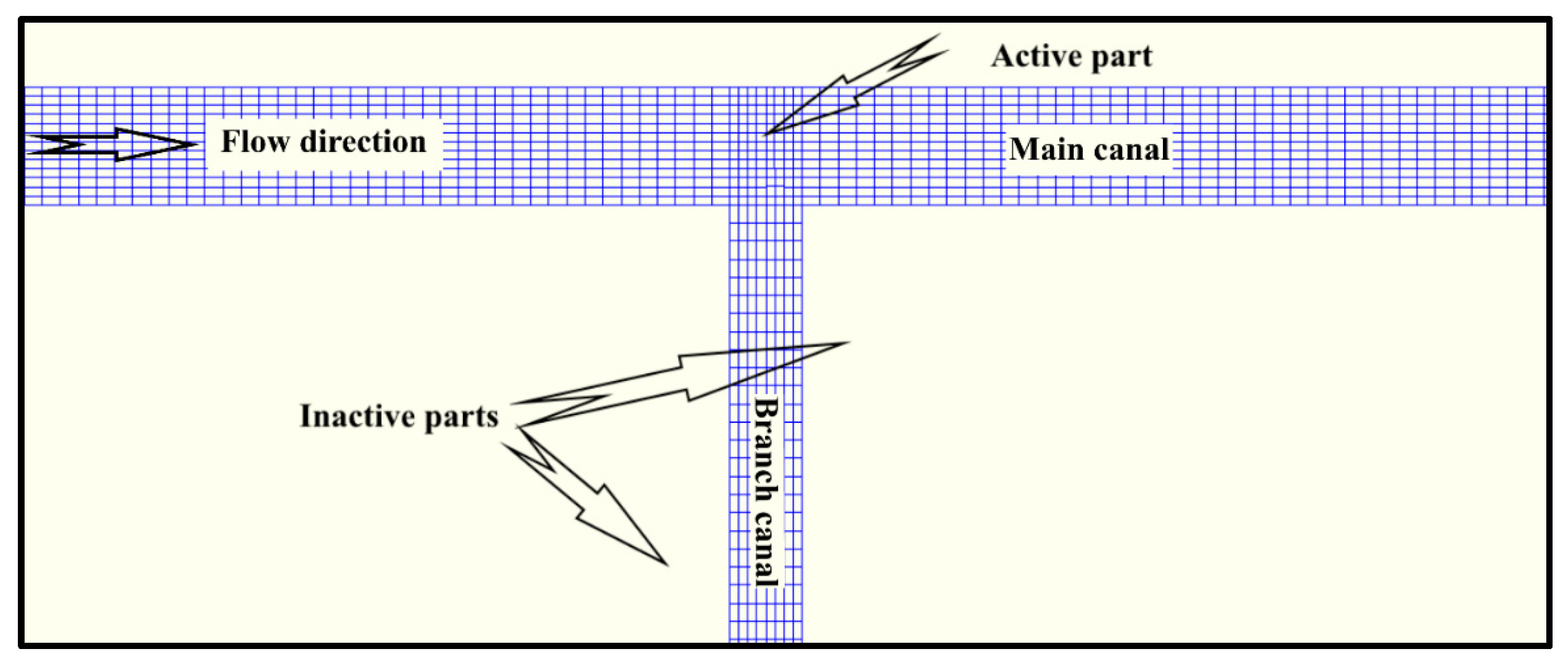
Structured grids with rectangular cells and areas are computationally efficient if aligned with long straight canals. However, in reality, a canal system consists of main canals and branches, with large ‘empty’ areas in between (Figure 1). These ‘empty’ inactive parts, which fall outside the area of interest, render the structured grids inefficient since the model domain includes large inactive parts taking up unnecessary computation time. Unstructured grids (or flexible mesh) can model irregular shapes that only include the active parts of the channel networks. However, these grids mostly consist of triangular cells which are not conducive for long canals, since they cannot be stretched in stream direction, leading to a higher number of triangular cells and hence longer simulation time. One possible solution is to use an unstructured grid with quadrilateral cells aligned with the flow direction along the canal (e.g., Delft3D FM or Mike FM). A more efficient solution is to use a structured grid with the domain decomposition (DD) tool available in Delft3D. This tool allows to divide the grid in separate parts that can be modelled and compiled. In this way inactive parts can be excluded, substantially reducing simulation time. The latter method, combining structured grids and domain decomposition, was used in this paper.
The Real-Time Control (RTC) tool enables changing weirs and gate settings during the simulation. This property can be activated in the Delft3D-FLOW input file by using the Rtcmod keyword. It allows simulating canal operation in which gates are opened and closed multiple times during the irrigation season. The morphological factor (Morfac or MF) feature in Delft3D further shortens the model running time and enables predictions of the morphologic developments in the medium term (months or seasons).
Comparing the three models Delft3D has all features necessary to simulate the effect of gate operation under scenarios of cohesive and non-cohesive sediment and their interaction. It is also open source and can handle non-steady flows.
Delft3D has been validated by Reference [21] for a series of simplified theoretical, laboratory and full-scale test cases. Furthermore, it was also validated against the results of prototype-scale measurements. A big advantage of numerical simulations is that there is no need to apply scale factors [21], unlike physical morphological models where sediment scaling is a major problem. Numerical morphological models can be tested directly against both the laboratory observations and prototype-scale observations.
So far the Delft3D model has been used primarily for rivers [23,24,25,26] and for estuaries [21,27] in 2D and/or 3D modes. The model has been used by Reference [16] for irrigation canals in both 2D and 3D. Running the model in 2D mode is to ensure better representation of the sediment processes and the large scale behavior with an acceptable simulation time period. Running the model in 3D mode provides information about the vertical and gives more details near structures.
2.1.2. Model Equations
Delft3D-FLOW solves the shallow water equations (derived from Reynolds-averaged Navier-Stokes equations for incompressible fluid under shallow water and Boussinesq assumptions). In the 3D simulations we have applied the k-ε turbulence closure model for vertical shear and a constant eddy viscosity model for horizontal shear. The sediment transport is split into both bedload and suspended load transport of non-cohesive sediments and suspended load of cohesive sediments; for the suspended load the advection-diffusion equation is solved with source and sink terms for sediment entrainment and deposition. The morphological change is computed based on an explicit integration of the bedload fluxes entering or leaving the grid cell plus the net deposition and entrainment.
For cohesive sediment fractions, the fluxes between the water phase and the bed are calculated with Partheniades-Krone formulations [28] for deposition and erosion [29]:
Erosion formula:
where:
: Erosion flux (kg m−2s−1);
: User-defined erosion parameter (kg m−2s−1);
: Erosion step function;
: Maximum bed shear stress (N/m2);
User-defined critical erosion shear stress (N/m2).
Deposition formula:
where:
: Average sediment concentration in the near bottom computational layer (kg/m3);
: Deposition flux (kg m−2s−1);
Deposition step function, Maximum bed shear stress (N/m2);
User-defined critical deposition shear stress (N/m2);
: Fall velocity (hindered) (m/s);
Zb: Depth down to the bed from a reference height (positive down) (m);
∆ Zb: Thickness of the bed layer (m).
The high value for tcr, d causes to be effectively equal to 1, therefore we can neglect this term from Equation (4) and the equation will be as below:
For the computation of the behavior of non-cohesive sediments, we have applied the approach developed by Reference [30]. Van Rijn [30] predicts the sediment transport as bed load and suspended load. A reference height (a) is used to differentiate between these loads; sediments transport below this reference height is treated as bedload transport and above it as suspended-load transport. The layer situated directly above the Van Rijn reference height is called the kmx-layer. The sediments in this layer which move between bed and water flow are modelled using sink and source terms.
The advection-diffusion equation solves the sink term implicitly, whereas the source term is solved explicitly. The concentration and concentration gradient at the bottom of the kmx-layer needs to be approximated, in order to determine the sink and source terms. The model assumes a standard Rouse-profile between the reference height (a) and the center of the kmx-layer:
In the Delft3D model, the reference height can be represented as:
where;
a = min [max {f × ks, 0.01 h}, 0.2h],
- A (l) = Rouse number
- a = Van Rijn’s reference height (m);
- C (l) = concentration of sediment fraction (l) (kg/m3);
- Ca (l) = reference concentration of sediment fraction (l) (kg/m3);
- f = user defined proportionality factor (−) (equals to 1);
- h = water depth (m);
- ks = roughness height (m);
- z = elevation above the bed (m).
Sink and source terms of the kmx-layer are subsequently calculated as follows:
Erosion formula:
where the first term is ) and the second term is ).
Deposition formula:
where:
- : Reference concentration of sediment fraction (l) (kg/m3);
- Average concentration of the kmx cell of sediment fraction (l) (kg/m3);
- : Settling velocity (m/s);
- ∆z: Difference in elevation between the center of the kmx cell, Van Rijn’s reference height: ∆z = zkmx − a (m);
- : First correction factor for sediment concentration (−);
- : Second correction factor for sediment concentration (−);
- : Sediment diffusion coefficient evaluated at the bottom of the kmx cell of sediment fraction (l) (−).
The reader is referred to Section 2.3.2 for the parameter settings used in this study.
2.2. Case Study
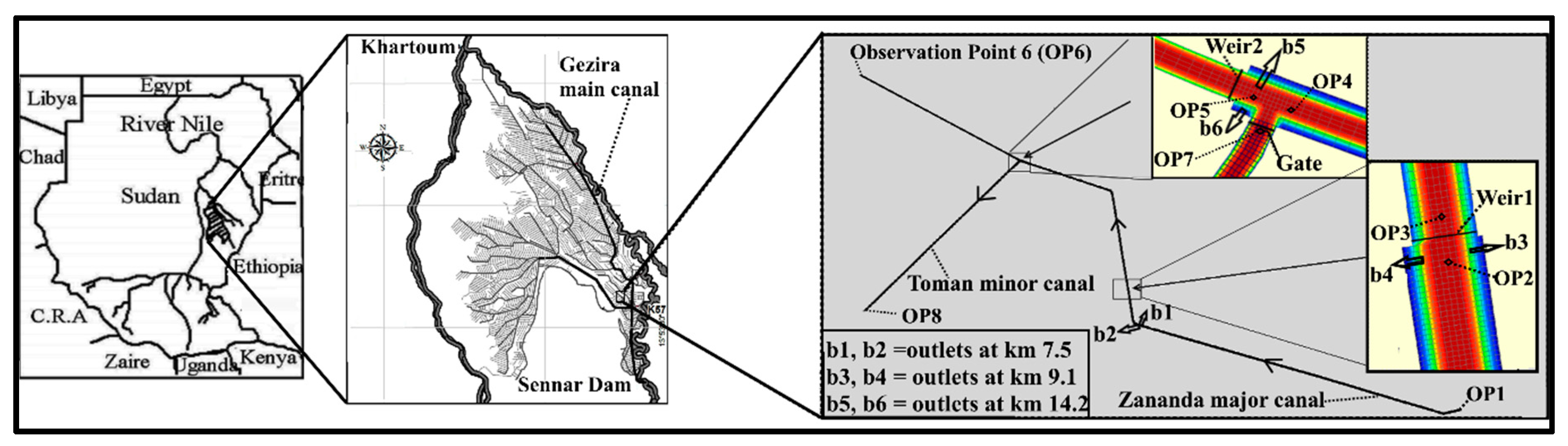
The Gezira Scheme is the largest irrigation scheme in Sudan, serving 8,800,000,000 m2 and taking water from the Blue Nile River which carries large amounts of sediment. Since its construction in 1920, the scheme suffers from sediment accumulation in the canals, representing a big challenge for the operation and maintenance. The annual costs of desilting were estimated at aroundUS $12 million [31]. The irrigation system consists of a network of main, major, minor and field canals. Two canals were selected for this study—the Zananda Major canal and Toman Minor canal, fed by the Zananda Canal. The Zananda canal is the first canal that takes water from the Gezira Main Canal by gravity irrigation [1] (Figure 2 and Figure 3).
The location of the off-take is 14°01′42″ N and 33°32′33″ E. The Zananda canal is 17 km long and provides water to seven minor canals in which irrigate about 8520 ha, one of these minor canals is Toman Minor canal. In Figure 2 the other minor canals are presented as outlets named b1, b2, b3, b4, b5 and b6. In the selected area, 75% of the sediment is silt and clay with grain sizes less than 0.063 mm (considered as cohesive sediment); the remaining 25% is fine sand as mentioned in the analysis of the bed materials done by Reference [1]. Reference [32] concluded that sediment is transported in suspension, based on sediment analysis. More details regarding the canal geometry and hydraulic parameters are presented in Table 2.
2.3. Model Setup
2.3.1. Grid Construction, Bathymetry and Other Parameters Assumptions
We constructed a grid for the Zananda major canal of 17 km long and 4 m wide from the inlet till the first contraction after the first weir where the width becomes 3 m till the end of the major canal. The grid for the Toman minor canal is 6.5 km long and 2 m wide with eight observation points as depicted in Figure 1. We followed the grid quality criteria of Delft3D with the orthogonality = 0.05 (i.e., cells are almost perpendicular to each other which proved the most suitable grid setting for reducing the Courant number that causes model instability in the course of the simulation) and smoothness = 1.2 for both M and N directions. The grid for the major canal contains 1125 and 14 cells in the M and N-direction respectively. The grid for the minor canal is 581 by 6 cells. For the 3D simulations, we have used five equidistant sigma-layers. The grid size for the long straight canal is 18 m. The more accurate mesh size of about 1 meter is used in important areas such as near the structure and near the minor canal. To reduce the computation time, the network domain is divided into the major grid domain and minor grid domain. The simulation results for both domains are compiled using the Domain Decomposition tool (DD), which reduces the simulation time to 40% of the total simulation time. Using the field data presented by Reference [1], we took the elevation of the upstream part of the Zananda major canal as a starting point and built the bathymetry of the remainder of the canal based on slope, length and canal geometry such as bed width, side slopes and roughness. We estimate the design discharge of the major canal as 5.5 m3/s, based on available data and field reports [1]. When canals are free of sediment, the flow is assumed to be as steady non-uniform flow during the time step (i.e., flow rates of the outlets do not change with time but depth of water varies with the location along the canal). For hydrodynamic reasons, the model is first executed without sediment to get a steady-state flow condition and check some crucial flow parameters such as velocity, water levels and the bed shear stress which is important in calculating the sedimentation and erosion of cohesive sediments. The steady-state flow condition was validated with results from the DUFLOW model following the method described in Reference [16]. Due to the absence of the detailed field data regarding velocity and bed shear stress, we compare Delft3D results of water level to the DUFLOW model, where the DUFLOW model was previously calibrated by Reference [1] against field data. Our water levels match those of DUFLOW within 5 cm. Reference [1] validated the DUFLOW model against field data, the water level of DUFLOW match the field data within 3 cm.
After adjusting uniform bed roughness and wall roughness for hydrodynamic parameters, we test the scenarios assuming the entrance of sediment at a constant rate, evaluating the morphological changes in the canal bed after a simulation time of three months and comparing the results to the initial bed levels.
2.3.2. Model Runs
The model was run for a simulation time of three months using a time-step of 0.6 s and a morphological factor (MF) of 10 using both 2D and 3D modes. The results of the 2D and 3D simulations look identical. In this paper, the graphs are based on the 3D simulations. The small-time step is chosen to avoid the Courant number exceeding 1.0 which would destabilize the model. The MF enables the computation of the morphodynamics together with the hydrodynamics. This MF was used to speed up the changes of bed morphology by 10 times per time step, which reduces the time by a factor of 10. Thus, simulating the effective morphological changes over 3 months requires only a simulation period of 9 days. The MF approach simplifies the model setup and operation in comparison with other approaches [33,34], in this way, the Delft3D model was capable to predict the changes in canal morphology over a long time span within small simulation time.
Two different computers were used in this study, One has simple specifications (dual-core Hp ProBook 6570b) and the other is a higher-performance computer is (quad core Hp Z Book15 G3); the latter reduced the simulation time by 40%. The CPU time was 3.5 days and 2days for 3D and 2D modelling respectively.
In this study the maximum concentration is assumed to be ( = 3 kg/m3 or 3000 ppm) for cohesive sediments, this concentration lies in the range of typical concentrations which are relevant for the Gezira Scheme [1]. As input data in Delft3D, the settling velocity (Ws) is set to 0.12 mm/s which corresponds to the Krone [35] formula for the aforementioned concentration. The value of the critical shear stress for erosion () is set to 1 N/m2. For the erosion parameter M l the default value of 0.0001 kg m−2s−1 is used. For the critical shear stress for deposition, the authors used tcr,d = 1000 N/m2.
The initial conditions are set as follows: water level = 34 m + (MSL) Mean Sea Level. The initial sediment concentration for each type of sediment equal to 0 kg/m3, the canal bed is erodible (movable) limited by the available amount of sediment. The initial sediment layer assumed to be 20 cm consist of 50% sandy material and 50% muddy material. The boundary conditions are: discharge equals 5.5 m3/s with sediment concentration is 3000 ppm and 100 ppm for cohesive and non-cohesive, respectively, as un upstream boundary condition. The downstream boundary condition for each canal was taken as Q-h relation which is based on the canal characteristics. For the other branches b1, b2, b6, they have been considered as only outflow, where each branch drags 0.5 m3/s of water from the major canal.
Other parameter values regarding non-cohesive sediment are D50 = 100 µm (fine sand) with a specific density of 2650 kg/m3. For the transport of non-cohesive sediment, we use the Van Rijn formula [30].
2.3.3. Morphological Comparison
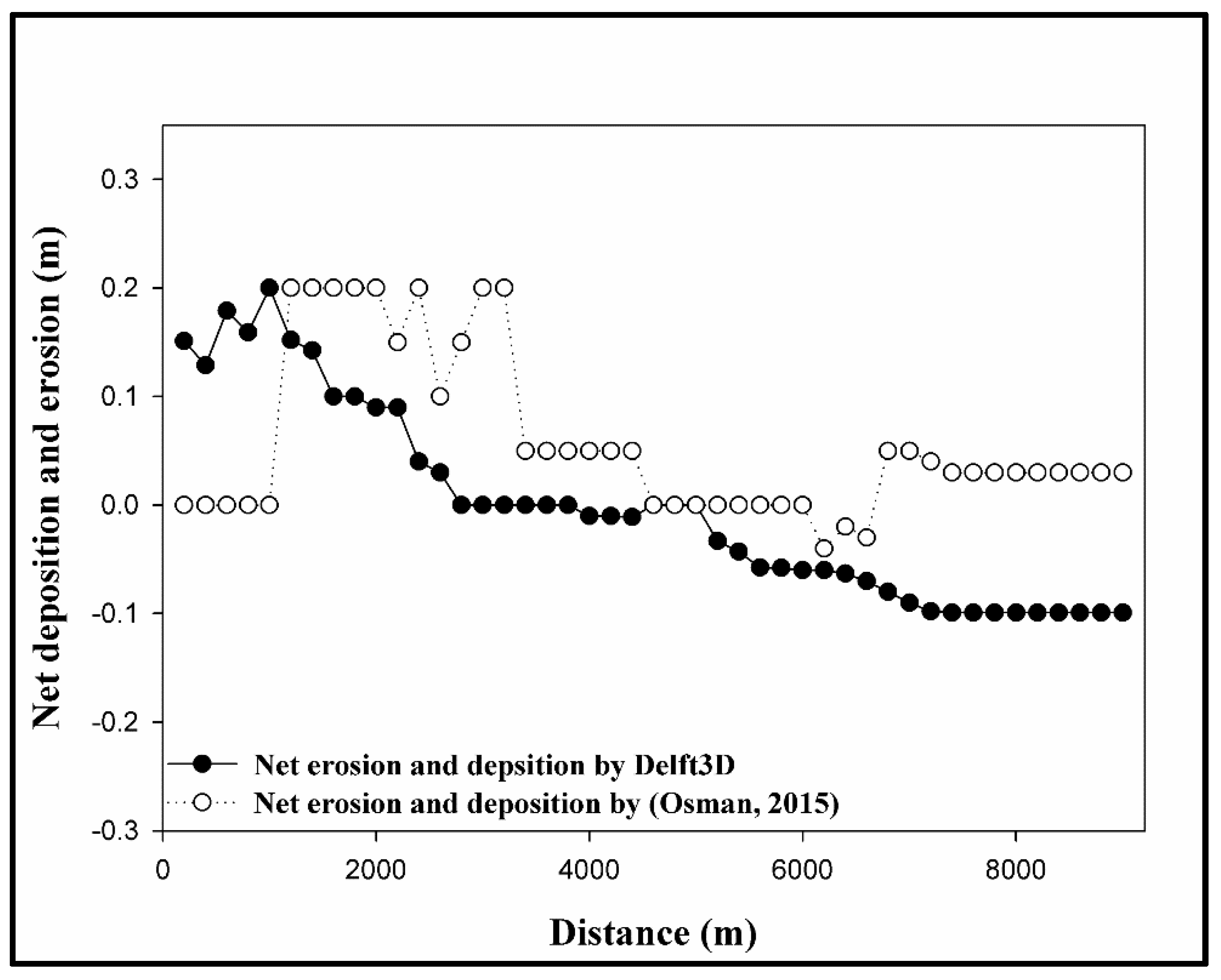
Reference [1] collected sediment data in the Gezira irrigation system in Sudan for the years 2011 and 2012. Given the difficulty of getting actual field data, we used the data from Reference [1] to verify the Delft3D model.
Figure 4 shows that the results obtained from Delft3D are qualitatively comparable with the field data measured by Reference [1], giving confidence that the Delft3D model is able to replicate field conditions. Delft3D results’ are also qualitatively comparable with the simulation results by Reference [1]. Observed differences in bed level are partly explained by differing modelling assumptions, the two simulation models use a different numerical technique. Reference [1] used a series of quasi-steady-state computations in her model, whereas Delft3D a dynamic model showing changes in time for flow characters like velocity, water depth and bed level changes due to sediment transport over time.
2.4. Scenarios
To assess the effect of operation and structures, we tested different scenarios regarding gate opening and height of weirs; weirs and gates influence the Delft3D computation by changing the through-flow area (2D) and (partially) blocking specific layers in the 3D model. The structures do not directly affect the sediment transport; the sediment transports are affected indirectly by the changed flow patterns. Gate opening and weir heights vary according to the scenario (Table 3) while sediment concentration and other parameters are kept constant during the simulation. Regarding the gate operation, the Real-time Control (RTC) module is applied because this tool allows us to open the gate fully, partially or fully close during the simulation.
3. Results
3.1. Reference Scenario
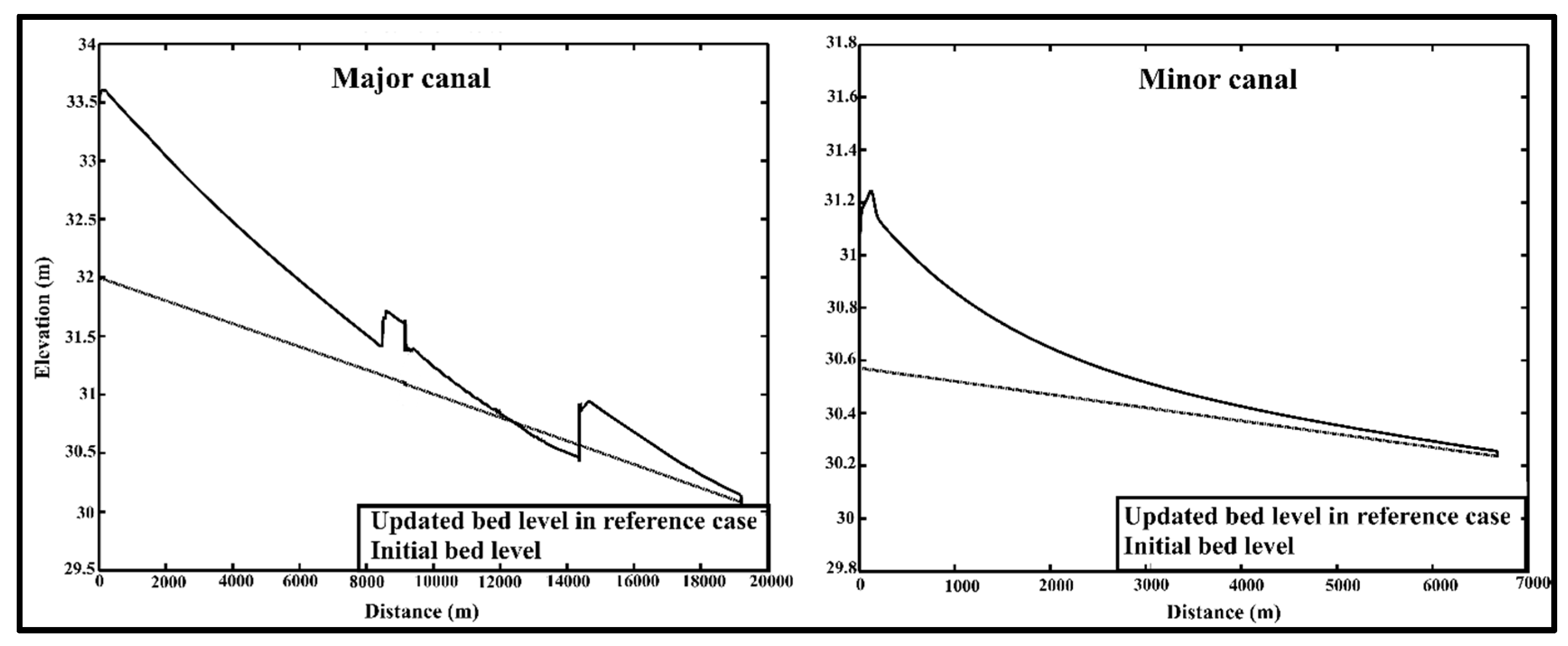
In the reference case, the gate in the Toman minor canal is fully opened while in the Zananda major canal, the height of both weirs is fixed at 0.3 m. During the simulation, sediments start depositing in the upstream part of the major canal (Figure 5). The cohesive sediment deposit gradually, distributed over the major canal while the non-cohesive sediments deposit mostly in the upstream of the canal. Because of the mixed sediment and interaction between cohesive and non-cohesive particles, the sedimentation pattern differs from the case of pure non-cohesive sediment. In the case of pure non-cohesive sediment, the heavy non-cohesive particles would rapidly deposit in the upstream the major canal. In the case of mixed sediment, some non-cohesive sediments are transported all the way to the downstream of the canal due to the interaction with the suspended cohesive particles.
In the canal stretch between 0 and 8 km, sediment deposition increases with time, with most accumulation (1.5 m) in the upstream of the major canal, the deposition in the first 8 km of the major canal consists mostly of non-cohesive sediments (Figure 5). With sufficient flow velocity, the transport capacity is sufficient to convey the sediments along the major canal. Just after 8 km in the vicinity of the first two outlets (b1 and b2) sediment locally accumulate. In the Delft3D model, we specify the amount of water drawn by the outlets (0.5 m3/s); the amount of suspended sediment removed by the outlet cannot be specified—it equals the amount of water withdrawn times the locally computed sediment concentration. After the outlet with less water remaining in the major canal, velocity and hence sediment transport capacity reduces leading to sediment deposition.
The sediment deposition gradually decreases until 9.1 km where the first weir and two outlets (b3 and b4) are located. One would expect the deposition to increase again due to the low velocity. However, due to the canal contraction close to these outlets the flow velocity increases. These two opposite effects more or less even each other out and the velocity remains approximately equal. As a result, the sediments continue to be moving downstream to 14.2 km. Just after 14.2 km, there is a big canal contraction causing erosion in the canal section upstream of the second weir due to the acceleration of flow velocity. The Toman minor canal and the last two outlets (b5 and b6) are located upstream of the second weir at 14.2 km. The outlets should decrease the velocity since they draw water from the major canal but because of the big canal contraction, velocity increases and erosion occurs. Thereafter the sediments continue to be transported till the end of the major canal.
In the minor canal, the gate is fully opened so the minor canal gets water carrying mostly cohesive sediments which deposit in the upstream of the minor canal (deposition reaches to 0.7 m). Since there is no structure disturbing their movement, the sediments are transported along the minor canal till the end (Figure 5), where the profile of the bed level shown is along the centerline (which is typically the deepest point of the cross-section). (For more details, see the PowerPoint contains movies showing the updating of morphology within the cross-section at different locations in the major canal. The link for the supplementary data is: https://drive.google.com/drive/folders/1Wlw9SQSqGgRBLxyIoQ5FOjqdYAmxXFVV?usp=sharing).
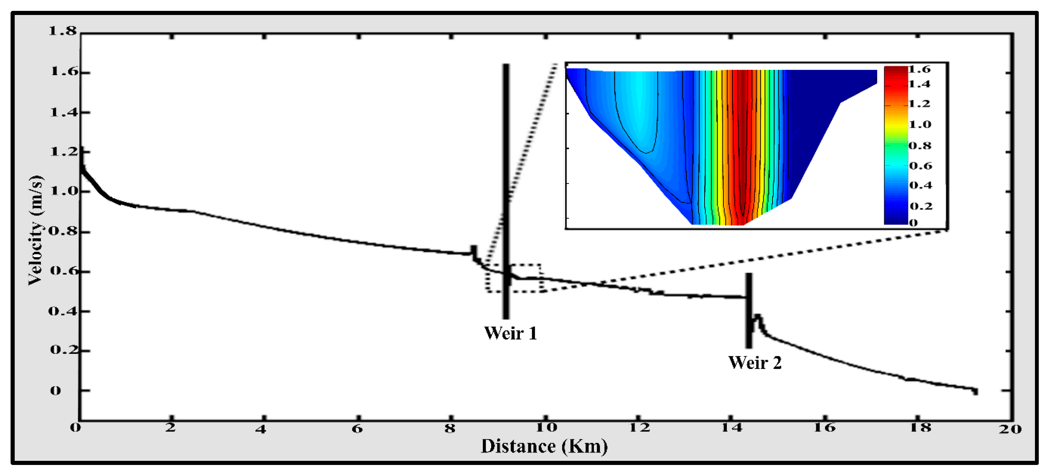
The flow velocity gradually reduces along the minor and major canals except above the weirs explaining the sedimentation and erosion patterns along the canals and within the cross-section (Figure 6).
The flow velocity (averaged over the cross-section) gradually reduces along the major canal (Figure 6). Within the cross-sections along the canal, the velocity distributions differ. For example, at the first weir, the average velocity is 0.6 m/s. The maximum velocity of 1.6 m/s occurs in the middle of the cross-section, while the velocity is at the sides is much less with 0 m/s close to both sidewalls. The left side has a higher velocity than the right side due to the asymmetric shape of the canal contraction and offtakes nearby. (For more details, see the PowerPoint contains other movies showing the behavior of velocity in the system near the diversion to minor canal. The link for the supplementary data is: https://drive.google.com/drive/folders/1Wlw9SQSqGgRBLxyIoQ5FOjqdYAmxXFVV?usp=sharing).
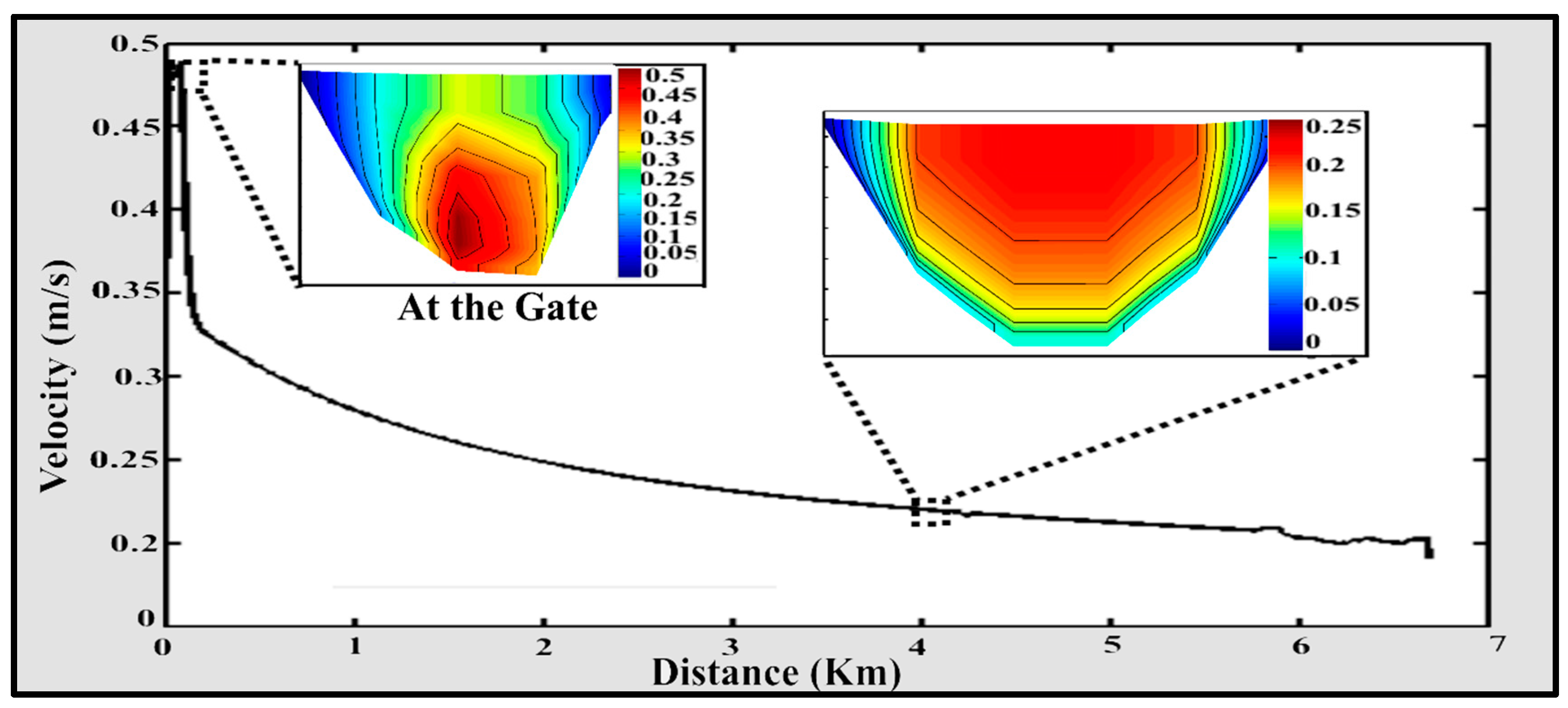
Also along the minor canal, the average flow velocity drops from 0.5 m/s upstream of the gate to 0.21 m/s at the downstream (Figure 7). Likewise, the flow velocity distributions within the cross-section vary with the highest velocities in the middle and lower velocities on both sides due to the roughness of the wall. In the downstream of the canal, the velocity distribution is logarithmic where higher velocities at the top layer of water and lower velocity near the bed. In the upstream near the gate, the water flows underneath the gate and the top layer velocity became less than the bottom layer velocity (Figure 7).
Due to differences in velocity distribution, sediment is distributed in an asymmetric way within the cross-sections of the major and minor canal. The sediment behavior is influenced by multiple factors such as the velocity, widening and contractions of the canals and bed shear stress.
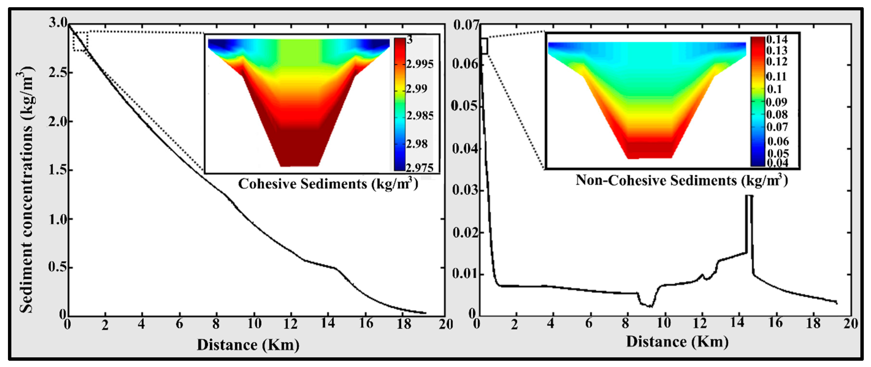
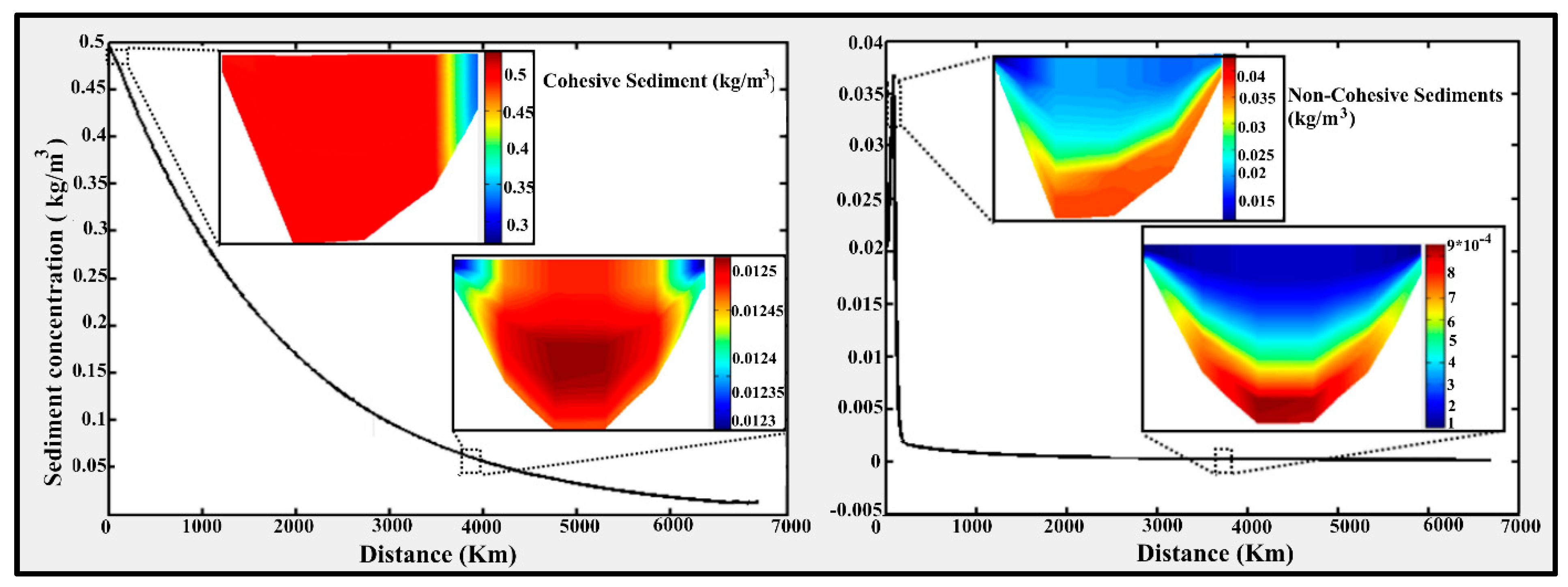
Figure 8 displays the difference in the deposition pattern between cohesive and non-cohesive sediments along the Zananda major canal. While cohesive sediments are gradually depositing along the major canal, the non-cohesive sediments are rapidly depositing in the first kilometers upstream of the canal with pronounced peaks and troughs in concentration near the weirs at 9 km and 14 km and canal contraction at 12.5 km. Non-cohesive sediments are deposited in the middle of the cross-section more than at both sides while the cohesive sediments are depositing almost equally in the middle and on both sides. In the case of pure cohesive sediments entering the irrigation system, most suspended sediments would be carried with the flow till the end of the major and minor canal. However, because in this case, the sediment is a mix of cohesive and non-cohesive, due to interaction with the heavier non-cohesive particles, some of the suspended cohesive particles start depositing in the upstream and middle of the canal stretches.
Figure 9 displays the difference in the deposition pattern between cohesive and non-cohesive sediments along the Toman minor canal. The same behavior will be there, where the cohesive sediments are gradually depositing along the minor canal, while the non-cohesive sediments are rapidly depositing at the beginning of the minor canal near the gate.
The cohesive sediment concentration in the minor canal is much higher than the non-cohesive sediment concentrations. This is the opposite of the situation in the major canal.
The deposition pattern between cohesive and non-cohesive sediments is different in the minor canal. Where cohesive sediments are gradually depositing along the minor canal, vice versa for the non-cohesive sediments. The pattern of depositing of cohesive and non-cohesive sediments within the cross-section is the same as in the major canal, with the highest concentrations at the bottom and sides.
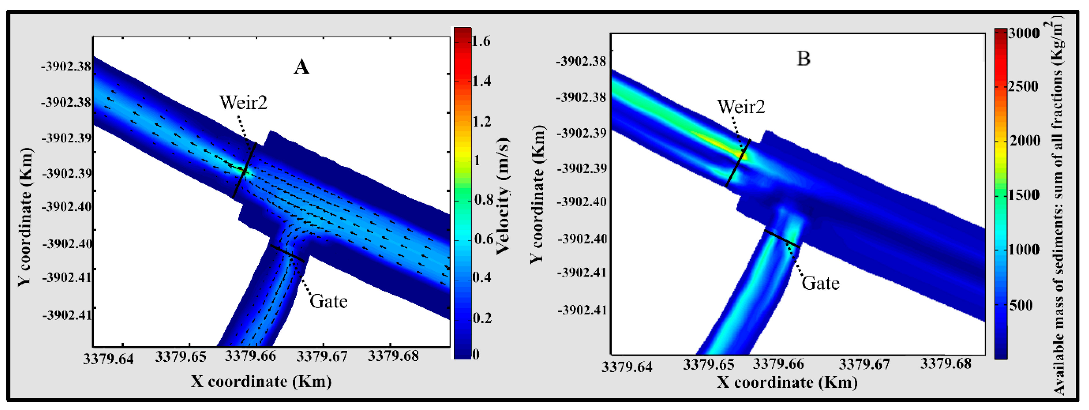
At the diversion to the minor canal, the velocity at the left side of the canal is reduced due to less water. Because of the subsequent reduction in velocity, a considerable amount of both non-cohesive and cohesive sediment is deposited, especially upstream the gate in the minor canal (Figure 10).
Figure 10 illustrates the effect of the velocity on the deposition and the transportation pattern of sediments. Panel (A) shows the reduced velocities at the right side of the canal after the diversion and the contraction. Panel (B) shows a higher deposition in these locations.
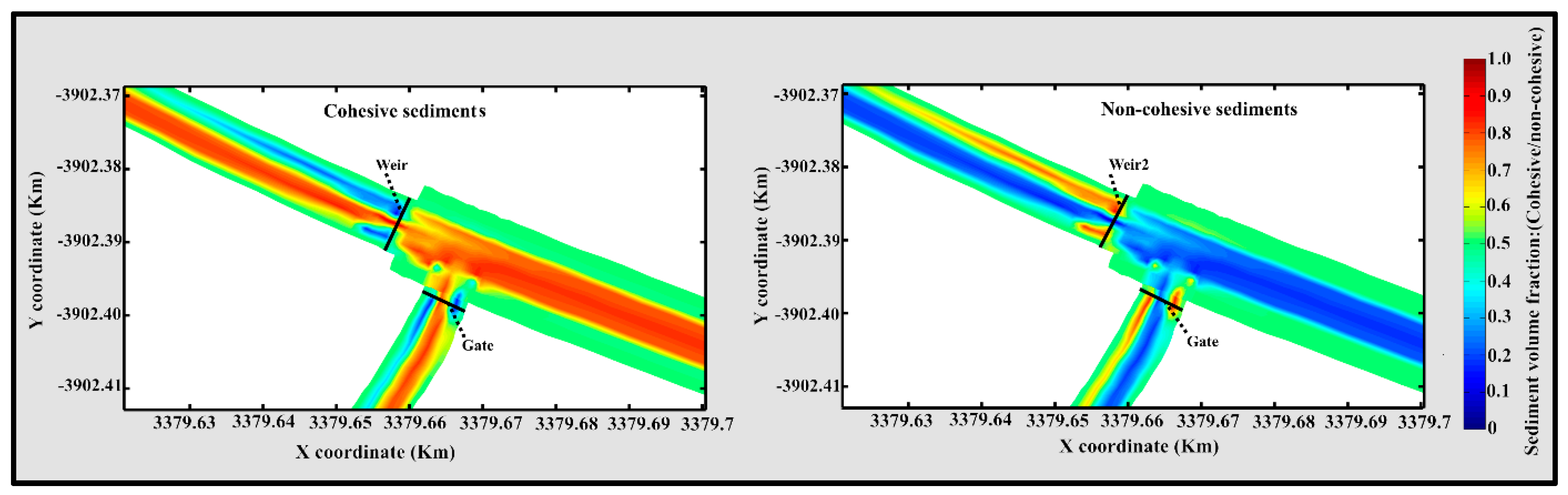
Acknowledging the asymmetric deposition patterns in the figures above, it can be noted the importance of using 2D/3D models to simulate sediment transport in the irrigation systems. Using Delft3D in this study proved useful in showing where the sediment is eroded or deposited and distributed along and within the cross-sections. Furthermore, Delft3D can show which kind of sediment is deposited where and in which quantities (Figure 11).
The deposition and distribution of both kinds of sediments are different where the large amounts of cohesive sediments pass through the minor canal (Figure 11). On the other hand, less non-cohesive sediments enter the minor canal (Figure 11) since it is rapidly deposited in the upstream part. (For more details, see the PowerPoint which contains movies showing the difference in distributions between the cohesive and non-cohesive sediment in the system, also movies showing the difference in the distribution of both sediments within the cross-section in the minor canal. The link for the supplementary data is: https://drive.google.com/drive/folders/1Wlw9SQSqGgRBLxyIoQ5FOjqdYAmxXFVV?usp=sharing).
3.2. Scenario 2: Effect of Weirs 1 and 2
3.2.1. Effect of the Upstream Weir (Weir 1)
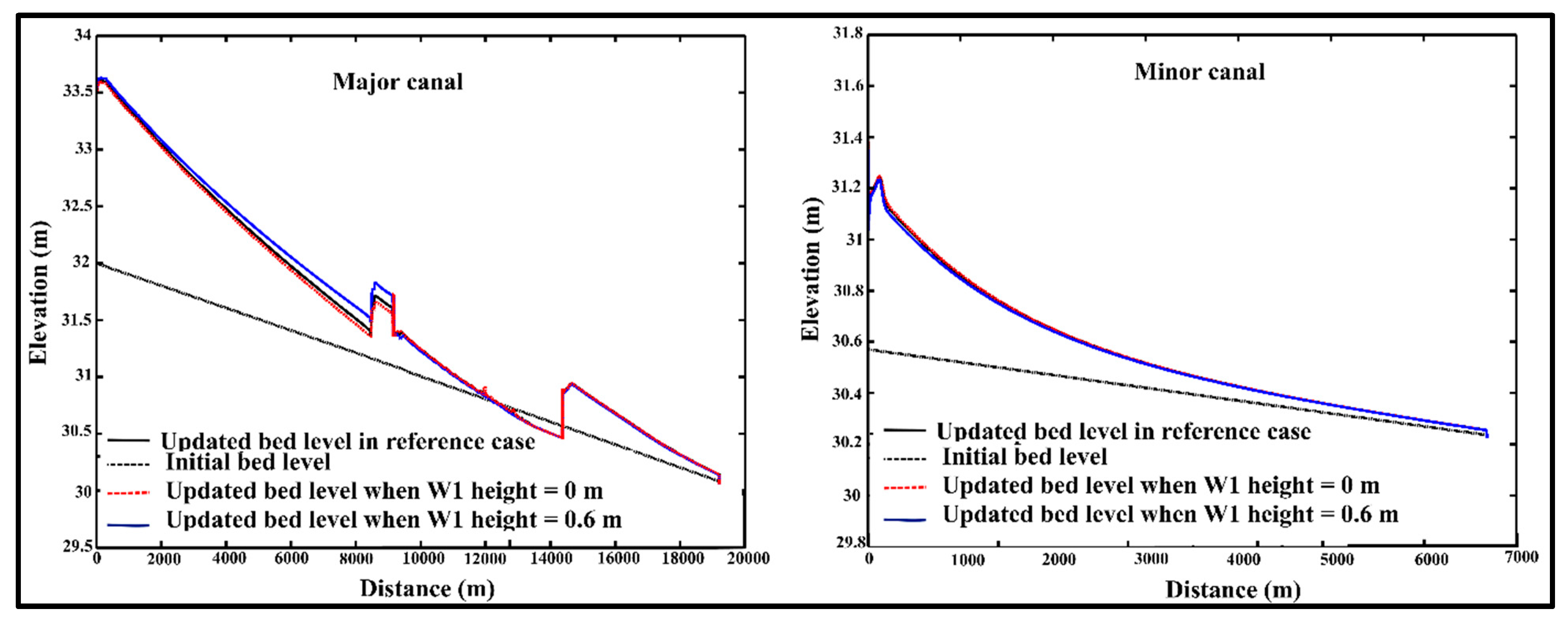
To see the effect of weir 1, we compare the sedimentation while reducing or raising the crest height of the weir. Raising the weir to 0.6 m increases the deposition slightly because of the obstruction of the water flow and creation of a backwater curve which leads to an increase in the water level and water depth. Combined with a constant discharge this leads to reduced velocity, reduced sediment transport capacity and hence more sediment deposition. This effect is noticeable only upstream of the weir and in the upstream part of the major canal, with a negligible effect on the downstream part of the major canal (Figure 12).
Lowering or removing weir 1 leads to reduce deposition because water moves freely without structures disturbing its movement so the sediment transport capacity is sufficient to move sediments. The effect is noticeable upstream of the weir and in the upstream part of the major canal, with a negligible effect in the downstream part of the major canal. The effect of the lowering or increasing of the weir height has little effect on the minor canal (Figure 12).
Changing the upstream weir settings reduces the sediment deposition significantly in the major canal while it has a negligible impact on the minor canal bed morphology (Figure 12).
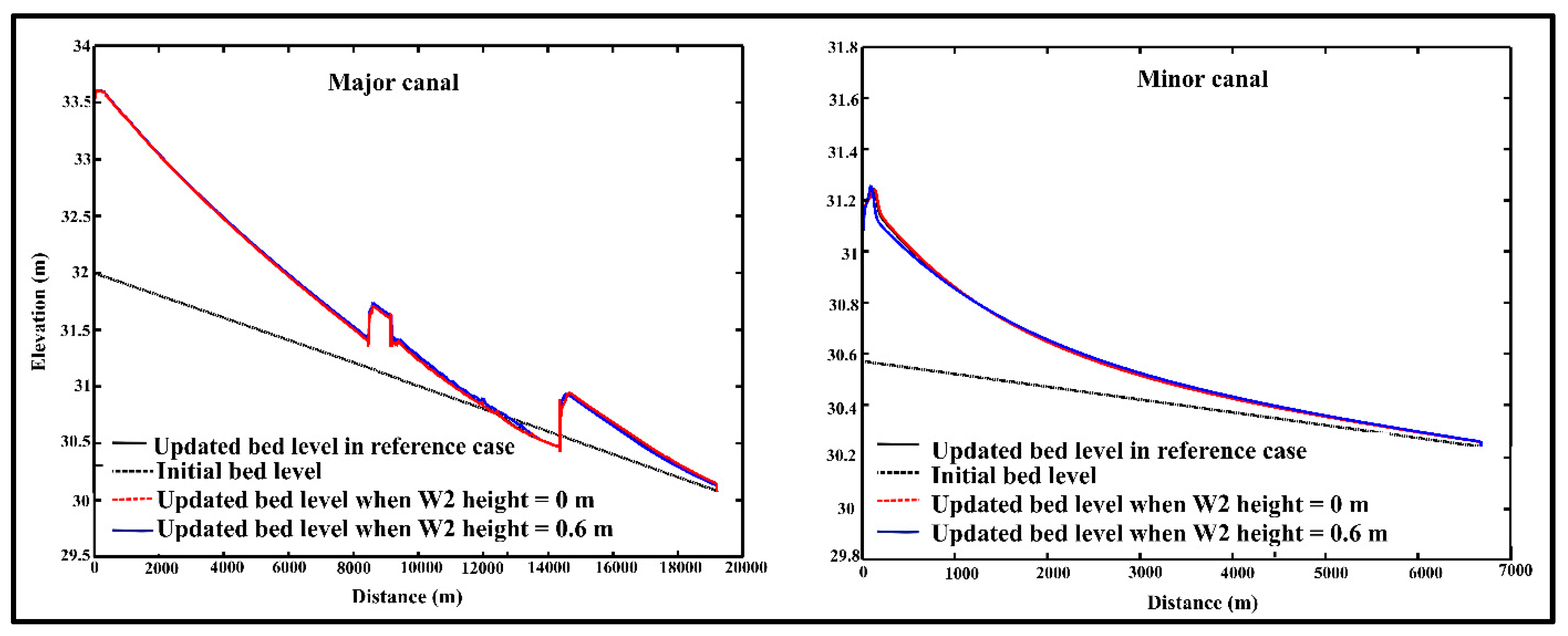
3.2.2. Effect of the Downstream Weir (Weir 2)
To evaluate the effect of weir 2, the weir has been raised and lowered in a similar way as weir 1 and compared the results with the reference case, the results shown in Figure 13 were too close. For this reason, changing the crest height of weir 2 has a little impact on sediment transport in the major and minor canals (Figure 13). Lowering and raising the downstream weir does not reduce the negative impacts of sedimentation, where the reduction in the deposition in both canals is very small.
3.2.3. Effect of Both Weirs
3.3. Effect of Gate Settings
3.3.1. Constant Gate Opening
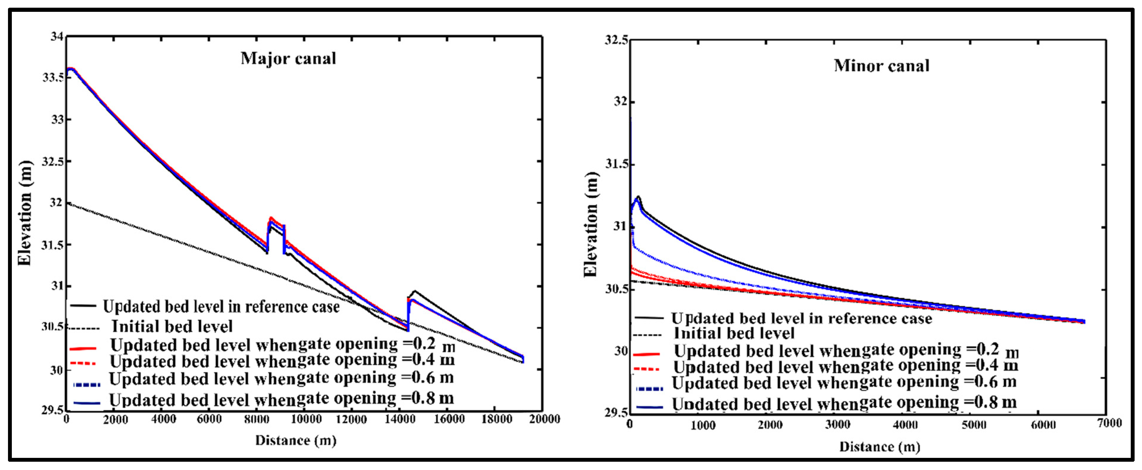
To see the effect of changing gate settings on sedimentation in the major and minor canal, the model was run with different gate openings to 0.2 m; 0.4 m; 0.6 m and 0.8 m and compared the modelling results with the reference case. Lowering the gate has a small impact on the major canal but substantially reduces sediment deposition in the minor canal. In case of gate openings equal to 0.2 m and 0.4 m sediment deposition almost fully blocks the canal reducing the flow into the minor canal to close to zero. The deposition in the first kilometers of the minor canal occurs due to the effect of weir 2. Due to the disturbance in the flow caused by weir 2 the water entering the minor canal is well mixed and loaded with sediment. The backwater curve due to weir 2 causes sediment deposition (Figure 5, Figure 6, Figure 7, Figure 8, Figure 9, Figure 10, Figure 11, Figure 12, Figure 13 and Figure 14). Lowering the gate reduces the deposition in the minor canal but at the same time, only a small amount of water can pass through the half-blocked canal which will not be sufficient to meet crop water requirements. Raising the gate can flush the sediment away.
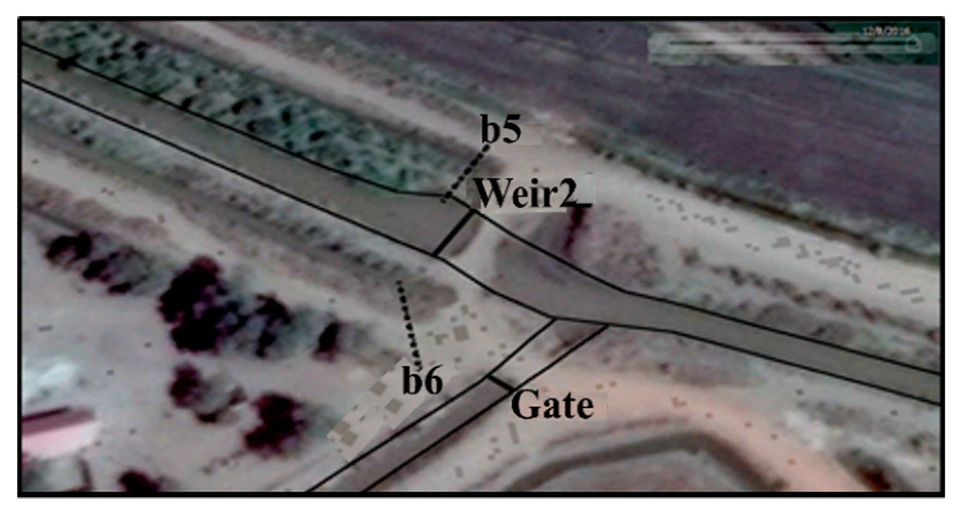
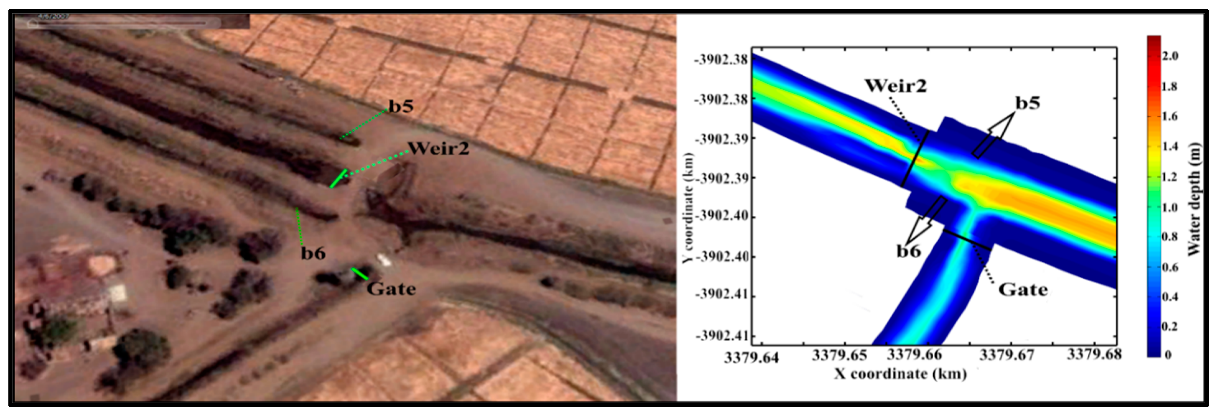
Figure 14 presents the effect of different fixed gate openings on the sediment deposition patterns in the major and minor canals. Reducing the gate height has a negligible impact on the major canal but a significant impact on sedimentation in the minor canal. However, reducing the gate also means less water entering the minor canal which may lead to insufficient water delivery to crops. Even though the gate setting of 0.8 m reduces the sediments deposition less than the other gate settings compared to the reference case, the larger opening ensures sufficient water to meet crop water requirements. The large sediment deposition is located at the upstream part of the minor canal and the subsequent narrowing of the canal is visible in the field and on Google Earth imagery (Figure 15) providing further evidence that modelling results mimic the actual situation.
3.3.2. Variable Gate Openings Following Different Operation Plans
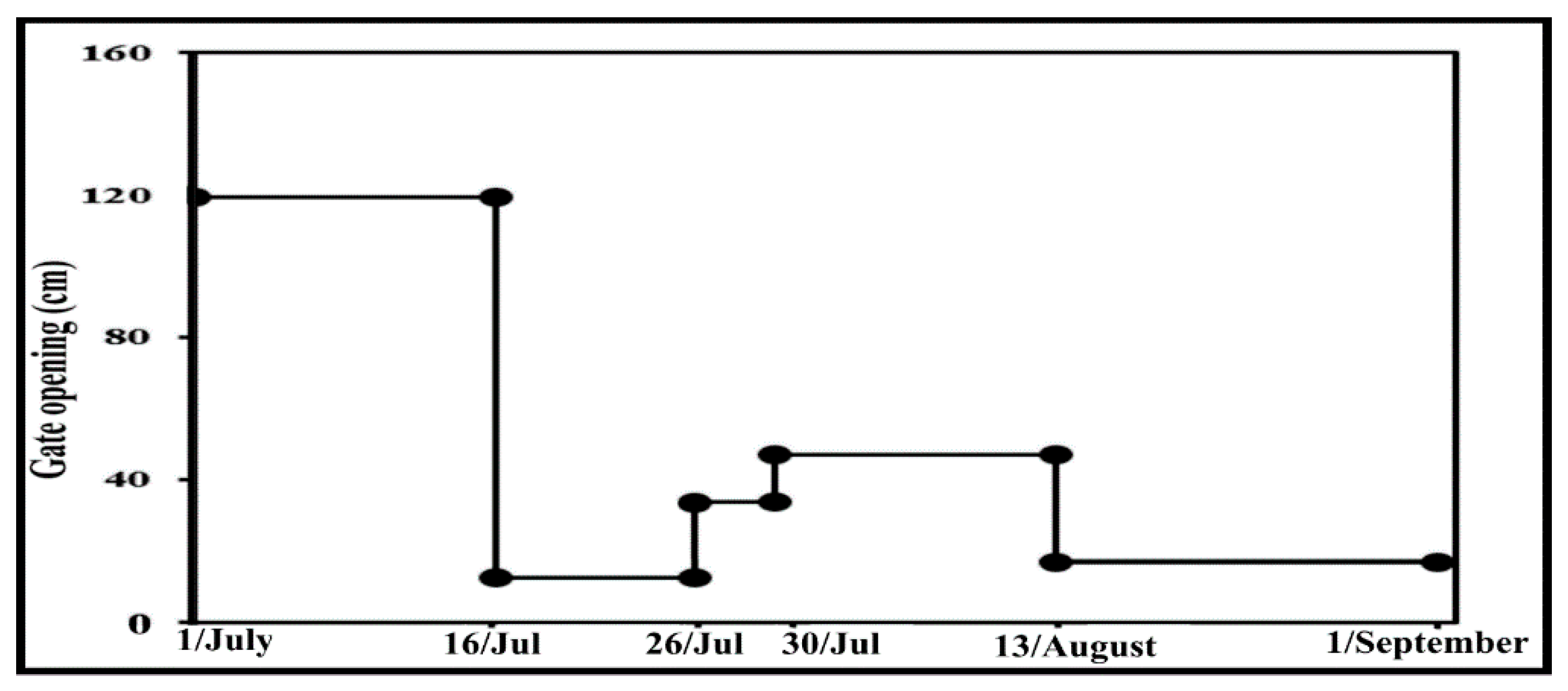
To test the impact of changing gate operation on the sedimentation in the canals, we formulate two different operation plans with different openings and time intervals based on the crop water requirements which change with crop growth stage. We prepare the first operation plan as shown in Figure 16 based on the data from Reference [1]. However, we simplified it by reducing the number of closing and opening the gate while keeping the same water distribution.
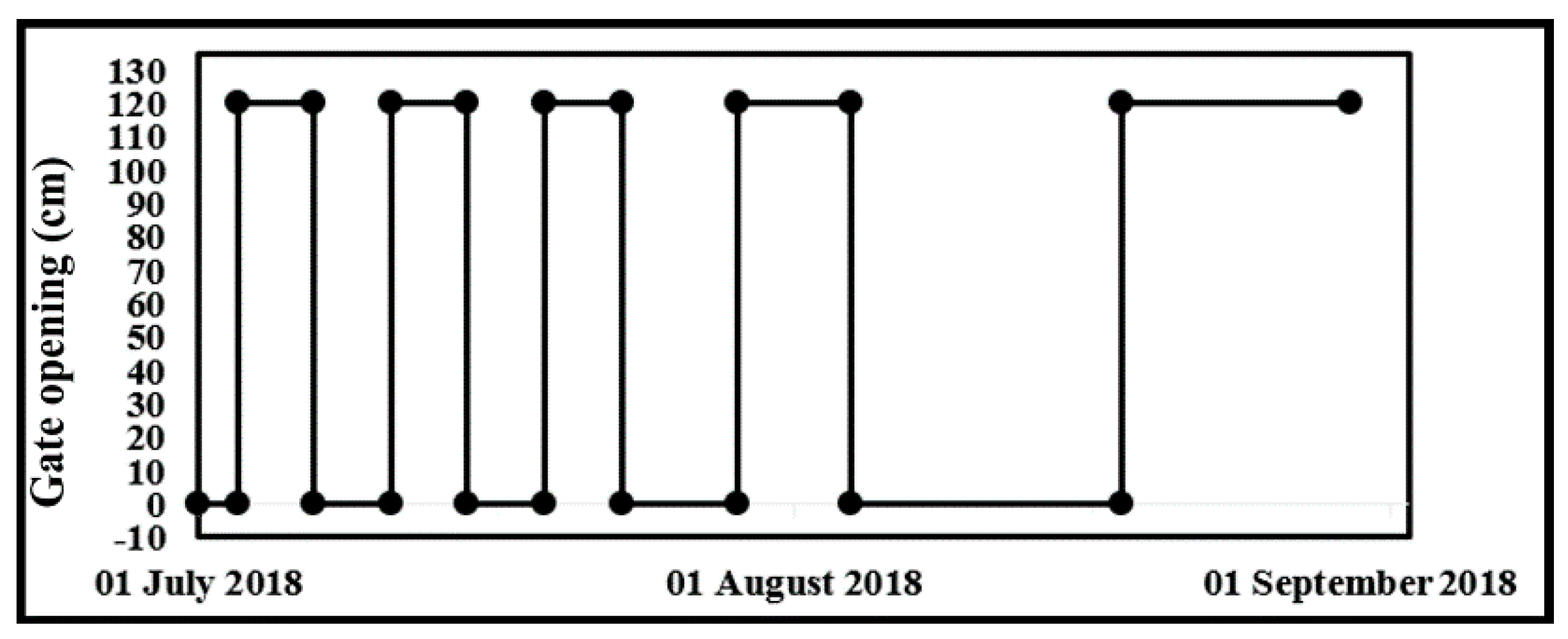
The second operation plan is prepared, by fully closing and opening the gate at varying time intervals taking into account crop water requirements (Figure 17).
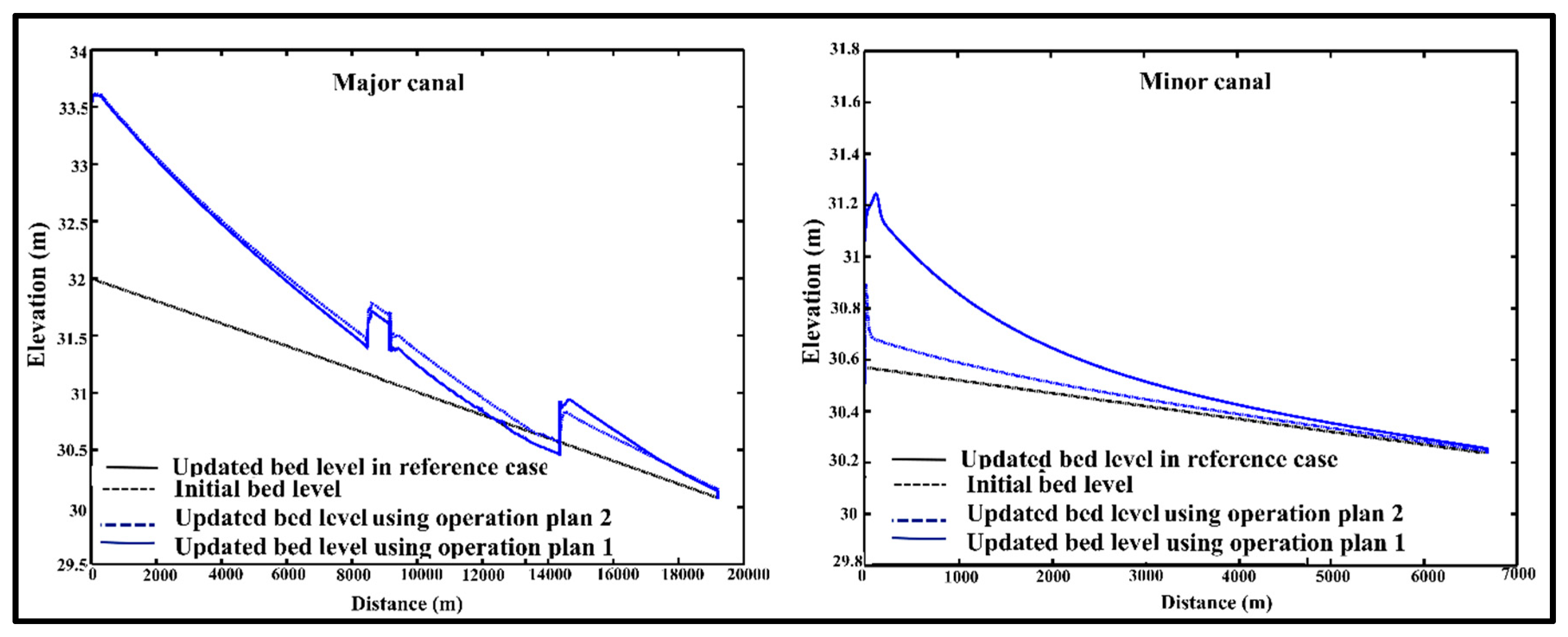
The first operation has a limited impact on sedimentation in the major and the minor canals as compared to the reference case. On other hand compared to the reference case operation plan 2 leads to a reduction in sediment deposition by half in the minor canal but limited impact on the major canal (Figure 18) while still meeting crop water requirements in a satisfactory manner. During the closure of the gate in the second operation plan the sediment accumulates near the gate and entrance to the minor canal. This is flushed away after fully opening the gate.
4. Discussion
Many factors affect the flow and the sediment movement in the irrigation canals. The offtakes diverting to the branch canals and field outlets catering for different water requirement, the changes in the canal geometry (contraction or widening) and other parameters all affect hydrodynamic and morphologic parameters that determine canal performance and capacity to transport sediment. In this paper, we illustrated how the location and the settings of weirs and gates do affect hydrodynamic and morphologic parameters.
Comparing scenarios to reduce sediment deposition in major and minor canals.
Table 4 summarizes the results of the scenarios related to the impacts of the weir and gate settings on the amount of cohesive and non-cohesive sediment in the major and minor canal. The last column provides a qualitative assessment of whether the weirs and gate settings in the scenario can meet the crop water requirements (CWR), based on the quantity of water that can be delivered to the outlet.
The upstream weir (w1 in Figure 1) has some impact on the deposition in the upstream of the major canal while in the downstream part and in the minor canal the effect is negligible. Raising the weir height disturbs the water flow and creates a backwater curve which leads to an increased water level and with constant discharge reduced velocity, ultimately resulting in reduced velocity, reduced sediment transport capacity and deposition of sediments. The downstream weir (w2) has less impact on both canals. Simultaneously lowering or raising both weirs resemble the results of the individual weir settings.
The results of scenario 3 with fixed gate settings reveal a relatively small impact on sedimentation in the major canal but a potentially large impact on the minor canal. Lowering the gate less than 0.6 m leads to substantial sediment deposition at the entrance and upstream of the minor canal. The sediment deposition in the first kilometer of the minor canal occurs because (1) due to the flow disturbance caused by downstream weir, water entering the minor canal carries the eroded sediment and (2) due to the small gate opening, less water flows in the minor canal leading to lower sediment carrying capacity and hence deposition further downstream. Over time this leads to a complete or partial blockage of the minor canal which will adversely affect the capacity to deliver sufficient water to meet crop water requirements. It should be noted however that the Delft3D model may not be able to accurately model the local sedimentation near the gate and subsequent canal blockage. We used the 3D hydrostatic mode with a limited resolution which cannot resolve the full 3D details of the local flow near structures. Modelling the flow and sediment dynamics at an even higher resolution would be desirable but is out of scope for operational reasons (mostly due to significantly increased simulation times).
Compared to the reference case the two operation plans (both based on crop water requirements but one with variable gate settings, the other with variable time intervals) have a limited impact on the major canal. However, the second operation plan reduces the sediment deposition in the minor canal by more than 50%. In this operation plan during the closure of the gate, sediment is deposited upstream the gate; the subsequent full opening of the gate flushes the sediment away. This could be incorporated as a convenient maintenance practice.
Table 4 shows that the best operation scenarios are (1) fixed gate opening at 0.8 m where crop water requirement can be met in a satisfactory manner while reducing sediment deposition in the minor canal (2) operation plan 2 with either fully closing or opening the gate at variable intervals. Sediment accumulated during gate closure can be flushed away by fully opening the gate.
Reference [17] found in one of her operation scenarios that reduced inflows during the high sedimentation period by 51% led to sediment reduction of 48%. In this paper in our first operation scenario, the same timings and gate settings were used as used by Reference [1] but kept the flow and (high) sediment concentration constant. The effect on sedimentation in the canals is small. Hence we conclude that in Osman’s scenario, the reduction of sediment-laden flow was the dominating factor in reducing sediment accumulation in the canal. Our second operation scenario shows the beneficial role of the intermittently opening and closing gate, even with high flow and sediment load. In this scenario, we assume constant sedimentation load temporally and spatially. In practice, sediment concentration in canals varies: some canals have very little or no sediments while others are suffering from high concentrations. Further, in some months sediment loads in the river are more severe than in others. Adjusting the timing of gate operation by closing the gate during periods of high sediment loads in the river to avoid sediments entering the minor canals can further reduce sediment problems.
The use of Delft3D for simulating sediment deposition in irrigation systems has significant advantages—(1) the 2D and 3D mode show where in the canal, longitudinal and in cross-sections, deposition and erosion takes place; (2) the RTC feature allows for including weirs and gates that can be adjusted during the simulation, to mimic gate operations; (3) the model handles non-steady flow well. This is important in irrigation systems where structures (gates and weirs) in the canal disturb the water flow; (4) the model can handle both cohesive and non-cohesive sediment and their interaction. The latter is important where irrigation systems use natural rivers which typically carry a mix of sediments. The Delft3D model helps to understand the mechanism of sediment transport, to predict the location, quantity and type of sediment accumulation under different operational scenarios. This information is essential for the design of operation and maintenance plans that will be effective in reducing sediment problems in irrigation systems.
As any other numerical model, Delft3D has limitations—(1) being developed for rivers, Delft3D does not simulate well the effects of sidewall roughness which makes the model inappropriate for narrow rectangular canals; (2) Delft3D and other 2D/3D hydrostatic models cannot predict local scour because vertical accelerations of the flow are ignored, turbulence modelling is limited and the sediment transport formulations are based on smooth flow conditions. For local scour detailed 3D non-hydrostatic models are needed with non-equilibrium sediment transport pickup and deposition processes [36]; (3) Delft3D does not take into consideration the effect of consolidation of (cohesive) sediments and makes no distinction between newly deposited fluffy material and old consolidated materials [37].
Finally there are two model implementation issues that need attention—(1) due to the much higher resolution than typical 1D models, simulation time can be extremely long, especially for large irrigation networks, despite useful tools such as Domain Decomposition, Flexible Mesh and Morphologic Factor, for example, in this study the cup time was 3.5 days and 2days for 3D and 2D modelling respectively; (2) the model implements the Q-h relationship as boundary condition in the downstream (i.e., water level as a function of the outflowing discharge Q). When the canal becomes dry and the water depth H drops to zero, this boundary does not reopen when the canal starts carrying water again. This situation frequently occurs in irrigation canals that are intermittently wet and dry depending on the water allocation plan. Most of these limitations are not insurmountable to solve since the model Delft3D is continuously developed further.
5. Conclusions
Efficient and well-executed canal operation plans can substantially improve hydraulic performance and reduce sediment problems which may lead to lower maintenance costs and as the result may increase crop production. This requires the proper operation of gates and finding the right balance between providing sufficient water for crop production and reducing sedimentation by the reduced sediment-laden flow. Our scenarios in the Gezira scheme in Sudan show how adjusting gate settings and varying timing of opening can be effective in reducing sedimentation in the secondary, distributary and field canals while meeting crop requirements in a satisfactory manner.
The Delft3D model, originally designed for rivers, was validated using measured field data from a previous study. The model was able to represent the actual condition (as shown in Figure 4, Figure 5, Figure 6, Figure 7, Figure 8, Figure 9, Figure 10, Figure 11, Figure 12, Figure 13, Figure 14 and Figure 15). The biggest advantages of the model (as compared to previous sediment studies) proved its ability to model both cohesive and non-cohesive sediments and its 2D mode. The latter allowed viewing flow parameters and sediments pattern within the cross-section, near offtakes, near gates and weirs and in the longitudinal direction. Determining the exact position of the sediment accumulation will help to reduce the maintenance costs and efforts and will also help the stakeholders to decide on the best operation to meet the crop water requirements while simultaneously minimizing sediment problems. Using a 3D model for cohesive and non-cohesive sediment, this study provides a substantial step forward in modelling the effect of structures on sediment behavior in irrigation canals and the use of gate operation to reduce sediment problems. Further studies are needed, in particular on the use of 3D models for large canal networks and with a better resolution around control and regulation structures. Running time and model stability are challenges here. Also, studies about the effect of gate operation with variable sediment concentrations will refine our scenarios.
Supplementary Materials
The PowerPoint and other helpful movies are available online at: https://drive.google.com/drive/folders/1Wlw9SQSqGgRBLxyIoQ5FOjqdYAmxXFVV?usp=sharing.
Author Contributions
S.A.T. carried out this research, conceived ideas and wrote the paper. B.J. took part in the implementation, analysis, guiding the ideas. F.X.S. participated in guiding the ideas. C.d.F. supervised and took part in the implementation, analysis, guiding the ideas and in the revising process.
Funding
This research received no external funding.
Acknowledgments
The Author would like to thank the Iraqi Ministry of Higher Education and Scientific Research and the Ministry of Water resources as well for funding my scholarship. Also, I would like to thank Deltares in Delft, the Netherlands for their technical help in providing the new version of the Delft3D and all modelling courses and workshops.
Conflicts of Interest
The authors declare no conflict of interest.
References
- Osman, I. Impact of Improved Operation and Maintenance on Cohesive Sediment Transport in Gezira Scheme, Sudan: UNESCO-IHE. Ph.D. Thesis, CRC Press, Boca Raton, FL, USA, 2015. [Google Scholar]
- Nawazbhutta, M.; Shahid, B.A.; Van Der Velde, E.J. Using a hydraulic model to prioritize secondary canal maintenance inputs: Results from Punjab, Pakistan. Irrig. Drain. Syst. 1996, 10, 377–392. [Google Scholar] [CrossRef]
- Belaud, G.; Baume, J.P. Maintaining equity in surface irrigation network affected by silt deposition. J. Irrig. Drain. Eng. 2002, 128, 316–325. [Google Scholar] [CrossRef]
- Jian, H.U. Study on mathematical modeling for non-uniform sediment transport in an irrigation district along the lower reach of the Yellow River. J. Chin. Inst. Water Resour. Hydropower Res. 2008, 1, 005. [Google Scholar]
- Jinchi, H.; Zhaohui, W.; Zhang, Q. A study on sediment transport in an irrigation district. In Proceedings of the 15th International Congress on Irrigation and Drainage, Hague, The Netherlands, 4–11 September 1993; pp. 1373–1384. [Google Scholar]
- Mendez, N.J. Sediment Transport in Irrigation Canals: UNESCO-IHE. Ph.D. Thesis, CRC Press, Boca Raton, FL, USA, 1998; p. 308. [Google Scholar]
- Paudel, K.P. Role of Sediment in the Design and Management of Irrigation Canals: Sunsari Morang Irrigation Scheme, Nepal: UNESCO-IHE. Ph.D. Thesis, CRC Press, Boca Raton, FL, USA, 2010. [Google Scholar]
- Depeweg, H.; Paudel, K. Sediment transport problems in Nepal evaluated by the SETRIC model. Irrig. Drain. 2003, 52, 247–260. [Google Scholar] [CrossRef]
- Munir, S. Role of Sediment. Transport in Operation and Maintenance of Supply and Demand Based Irrigation Canals: Application to Machai Maira Branch Canals: UNESCO-IHE. Ph.D. Thesis, CRC Press, Boca Raton, FL, USA, 2011. [Google Scholar]
- Celik, I.; Rodi, W. Modeling suspended sediment transport in nonequilibrium situations. J. Hydraul. Eng. 1988, 114, 1157–1191. [Google Scholar] [CrossRef]
- Liu, W.C.; Hsu, M.H.; Kuo, A.Y. Modelling of hydrodynamics and cohesive sediment transport in Tanshui River estuarine system, Taiwan. Mar. Pollut. Bull. 2002, 44, 1076–1088. [Google Scholar] [CrossRef]
- Lopes, J.; Dias, J.; Dekeyser, I. Numerical modelling of cohesive sediments transport in the Ria de Aveiro lagoon, Portugal. J. Hydrol. 2006, 319, 176–198. [Google Scholar] [CrossRef]
- Guan, W.B.; Wolanski, E.; Dong, L.-X. Cohesive sediment transport in the Jiaojiang River estuary, China. Estuar. Coast. Shelf Sci. 1998, 46, 861–871. [Google Scholar] [CrossRef]
- Van Rijn, L.C.; Van Rossum, H.; Termes, P. Field verification of 2-D and 3-D suspended-sediment models. J. Hydraul. Eng. 1990, 116, 1270–1288. [Google Scholar] [CrossRef]
- Wu, Y.; Falconer, R.; Uncles, R. Modelling of water flows and cohesive sediment fluxes in the Humber Estuary, UK. Mar. Pollut. Bull. 1999, 37, 182–189. [Google Scholar] [CrossRef]
- Theol, A.S.; Jagers, B.; Suryadi, F.; de Fraiture, C. The use of Delft3D for Irrigation Systems Simulations. Irrig. Drain. 2019, 68, 318–331. [Google Scholar] [CrossRef]
- Osman, S.I.; Schultz, B.; Osman, A.; Suryadi, F. Effects of different operation scenarios on sedimentation in irrigation canals of the Gezira Scheme, Sudan. Irrig. Drain. 2017, 66, 82–89. [Google Scholar] [CrossRef]
- Theol, S.; Jagers, B.; Suryadi, F.; De Fraiture, C. The use of 2D/3D models to show the differences between cohesive and non-cohesive sediments in irrigation systems. Submitt. Am. J. Irrig. Drain. Eng. (ASCE) 2019. forthcoming. [Google Scholar]
- Lesser, G.R.; Roelvink, J.V.; Van Kester, J.; Stelling, G. Development and validation of a three-dimensional morphological model. Coast. Eng. 2004, 51, 883–915. [Google Scholar] [CrossRef]
- Morianou, G.G.; Kourgialas, N.N.; Karatzas, G.P.; Nikolaidis, N.P. Hydraulic and sediment transport simulation of Koiliaris River using the MIKE 21C model. Procedia Eng. 2016, 162, 463–470. [Google Scholar] [CrossRef] [Green Version]
- Lesser, G.R. An Approach to Medium-Term Coastal Morphological Modelling: UNESCO-IHE. Ph.D. Thesis, CRC Press, Boca Raton, FL, USA, 2009; p. 255. [Google Scholar]
- Villaret, C.; Hervouet, J.-M.; Kopmann, R.; Merkel, U.; Davies, A.G. Morphodynamic modeling using the Telemac finite-element system. Comput. Geosci. 2013, 53, 105–113. [Google Scholar] [CrossRef]
- Kemp, L. The Evolution of Sandbars along the Colorado River Downstream of the Glen Canyon Dam. Master’s Thesis, Delft University of Technology, Delft, The Netherlands, 2010. [Google Scholar]
- Gebrehiwot, K.A.; Haile, A.M.; De Fraiture, C.; Chukalla, A.D.; Tesfa-alem, G.E. Optimizing flood and sediment management of spate irrigation in Aba’ala Plains. Water Resour. Manag. 2015, 29, 833–847. [Google Scholar] [CrossRef]
- Flokstra, C.; Jagers, H.R.A.; Wiersma, F.E.; Mosselman, E.; Jongeling, T.H.G. Numerical Modelling of Vanes and Screens; Development of Vanes and Screens in Delft3D-MOR; Delft University of Technology: Delft, The Netherlands, 2003. [Google Scholar]
- De Jong, J. Modelling the Influence of Vegetation on the Morphodynamics of the River Allier. Master’s Thesis, Technology University of Delft, Delft, The Netherlands, 2005. [Google Scholar]
- Van der Wegen, M.; Jaffe, B.; Roelvink, J. Process-based, morphodynamic hindcast of decadal deposition patterns in San Pablo Bay, California, 1856–1887. J. Geophys. Res. Earth Surf. 2011, 116. [Google Scholar] [CrossRef] [Green Version]
- Partheniades, E. Erosion and deposition of cohesive soils. J. Hydraul. Div. 1965, 91, 105–139. [Google Scholar]
- Deltares. Delft3D-Flow User Manual; Deltares: Delft, The Netherlands, 2016; Available online: https://oss.deltares.nl/documents/183920/185723/Delft3D-FLOW_User_Manual.pdf (accessed on 28 May 2016).
- Van Rijn, L.C. Principles of Sediment Transport in Rivers, Estuaries and Coastal Seas; Aqua Publications: Amsterdam, The Netherlands, 1993; Volume 1006. [Google Scholar]
- Gismalla, Y.A. Sedimentation problems in the Blue Nile reservoirs and Gezira scheme: A review. Gezira J. Eng. Appl. Sci. 2009, 4, 1–12. [Google Scholar]
- Osman, I.S.; Schultz, B.; Osman, A.; Suryadi, F. Simulation of Fine Sediment Transport in Irrigation Canals of the Gezira Scheme with the Numerical Model FSEDT. J. Irrig. Drain. Eng. 2016, 142. [Google Scholar] [CrossRef]
- Li, L. A Fundamental Study of the Morphological Acceleration Factor. Available online: http://resolver.tudelft.nl/uuid:2780f537-402b-427a-9147-b8652279a83e (accessed on 23 August 2010).
- Roelvink, D.; Boutmy, A.; Stam, J.-M. A simple method to predict long-term morphological changes. Coast. Eng. Proc. 1998, 1. [Google Scholar] [CrossRef]
- Krone, R.B. Flume Studies of the Transport of Sediment in Estuarial Shoaling Processes; University of California: Oakland, CA, USA, 1962. [Google Scholar]
- Thanh, N.V.; Chung, D.H.; Nghien, T.D. Prediction of the local scour at the bridge square pier using a 3D numerical model. Open J. Appl. Sci. 2014, 4, 34. [Google Scholar] [CrossRef] [Green Version]
- Zhou, Z.; van der Wegen, M.; Jagers, B.; Coco, G. Modelling the role of self-weight consolidation on the morphodynamics of accretional mudflats. Environ. Model. Softw. 2016, 76, 167–181. [Google Scholar] [CrossRef]
Figure 1.
The active and inactive parts in the computational domain.

Figure 2.
Scheme of the Zananda Major Canal and Toman minor canal, labels b1–b6 indicate the locations of the outlets while labels OP1–OP8 indicate the locations of the observation points.
Figure 2.
Scheme of the Zananda Major Canal and Toman minor canal, labels b1–b6 indicate the locations of the outlets while labels OP1–OP8 indicate the locations of the observation points.

Figure 3.
Location of Toman minor canal (Google Earth).

Figure 4.
Comparing results from the Delft3D model with field and simulation data obtained from Reference [1].
Figure 4.
Comparing results from the Delft3D model with field and simulation data obtained from Reference [1].

Figure 5.
Sedimentation and erosion of sediments in the reference case.

Figure 6.
Flow velocity along the Zananda major canal and in the cross-section near the first weir.

Figure 7.
Velocity distribution in the Toman minor canal at different cross-sections.

Figure 8.
Distribution patterns of cohesive and non-cohesive sediments in Zananda major canal at different cross-sections.
Figure 8.
Distribution patterns of cohesive and non-cohesive sediments in Zananda major canal at different cross-sections.

Figure 9.
Sediment distribution patterns of cohesive and non-cohesive sediments in the Toman minor canal at different cross-sections.
Figure 9.
Sediment distribution patterns of cohesive and non-cohesive sediments in the Toman minor canal at different cross-sections.

Figure 10.
The relation between the velocity (A) and the amount of sediments (B) deposited at the diversion to the minor canal.
Figure 10.
The relation between the velocity (A) and the amount of sediments (B) deposited at the diversion to the minor canal.

Figure 11.
The difference in sediment distribution between the cohesive and non-cohesive sediments at the diversion.
Figure 11.
The difference in sediment distribution between the cohesive and non-cohesive sediments at the diversion.

Figure 12.
The effect of the upstream weir on sedimentation in the major canal (left panel) and the minor canal (right panel).
Figure 12.
The effect of the upstream weir on sedimentation in the major canal (left panel) and the minor canal (right panel).

Figure 13.
The effect of the downstream weir on sedimentation in the major canal (left panel) and the minor canal (right panel).
Figure 13.
The effect of the downstream weir on sedimentation in the major canal (left panel) and the minor canal (right panel).

Figure 14.
The effect of different fixed gate openings in time on sedimentation in the major canal (left panel) and the minor canal (right panel).
Figure 14.
The effect of different fixed gate openings in time on sedimentation in the major canal (left panel) and the minor canal (right panel).

Figure 15.
Comparing the Delft3D model results with actual field conditions as captured by Google Earth.
Figure 15.
Comparing the Delft3D model results with actual field conditions as captured by Google Earth.

Figure 16.
Operation plan with varying openings and time intervals based on crop water requirements.
Figure 16.
Operation plan with varying openings and time intervals based on crop water requirements.

Figure 17.
Operation plan with fully opening or closing the gate but with varying time intervals taking into account changing crop water requirements.
Figure 17.
Operation plan with fully opening or closing the gate but with varying time intervals taking into account changing crop water requirements.

Figure 18.
Effect of gate operation plan (in which the gate is either fully closed or opened at different time intervals) on sedimentation of the major canal (left panel) and left canal (right panel).
Figure 18.
Effect of gate operation plan (in which the gate is either fully closed or opened at different time intervals) on sedimentation of the major canal (left panel) and left canal (right panel).


Table 1.
Comparison between different models.
| Features Available | Delft3D | Telemac | Mike 21 |
|---|---|---|---|
| Grid construction | Structured with DD * | ||
| Unstructured (FM) ** | FM | FM | |
| Simulating: Cohesive sediments | Yes | No | Yes |
| Simulating: Non-cohesive sediments | Yes | Yes | Yes |
| Open-source | Yes | Yes | No |
| RTC *** | Yes | No | Yes |
* DD: domain decomposition, ** FM: flexible mesh, *** RTC: real-time control.
Table 2.
Geometric data.
| Property | Major Canal | Minor Canal |
|---|---|---|
| Canal length | 17 km | 6.5 km |
| Canal width | 4 m from (0–9.1) km 3 m from (9.1–17) km | 2 m |
| Canal bank height | 5 m | 4 m |
| Roughness (n) | 0.029 | 0.029 |
| Slope | 0.0001 | 0.00005 |
| Side slope | 1:2 from (0–14.2) km1:1 from (14.2–17) km | 1:1.5 |
| Structures | Weir 1 and weir2 with a height of 0.3 m, length of 3 m. | Gate fully opened |
Table 3.
Scenarios in the study.
| Scenario | Description | Remarks |
|---|---|---|
| 1. Reference case | Full open gate and fixed weirs’ heights. | Gate fully opened; w1, w2 with fixed height at 0.3 m. |
| 2. Effect of the weirs | a. Setting of the upstream weir height | Gate fully opened; lowering or removing, raising the weir (0 m, 0.6 m). |
| b. Setting of the downstream weir height | ||
| c. Setting of both weirs. | ||
| 3. Effect of the gate | a. gate setting with constant openings | Lowering the gate (0.2 m–0.8 m); weir1 and weir2 with fixed height at 0.3 m. |
| b. gate setting with variable openings | Operation plans for the gate; weir1 and weir2 with fixed height at 0.3 m. |
Table 4.
The impacts of operation in the sediment deposition as compared to the reference scenario.
| Scenarios | Description | Major Canal | Minor Canal | Meeting | |||
|---|---|---|---|---|---|---|---|
| Cohesive | Non-Cohesive | Cohesive | Non-Cohesive | CWR | |||
| Scenario 2 (Weir effects) | Upstream Weir | w1 = 0 | −0.5% | −0.5% | No change | No change | 3 |
| w1 = 0.6 | +1% | +1% | +2% | +2% | 2 | ||
| Downstream Weir | w2 = 0 | No change | No change | +3% | +3% | 2 | |
| w2 = 0.6 | No change | No change | −1.2% | −1.2% | 3 | ||
| Both Weirs | w1 = w2 = 0 | −2% | −2% | +3% | +4% | 2 | |
| w1 = w2 = 0.6 | +1% | +1% | −1.1% | −1.1% | 2 | ||
| Scenario 3 (Gate effects) | Fixed gate height | g = 0.2 | +4% | +4% | Block | Block | 0 |
| g = 0.4 | +4% | +4% | Block | Block | 0 | ||
| g = 0.6 | +3% | +3% | Partially block | Partially block | 1 | ||
| g = 0.8 | +1% | +1% | −19% | −19% | 2 | ||
| Operation | Plan1 | −0.1% | −0.1% | No change | No change | 3 | |
| Plan2 | +3% | +3% | −54% | −55% | 2 | ||
where (−) denotes a reduction and (+) an increase in sediments deposition as compared to the reference scenario; CRW = crop water requirement is assessed qualitatively in which 0 = no water, 1 = insufficient water for crops, 2 = more or less sufficient water to satisfy CWR, 3 more than sufficient water to satisfy CWR.
© 2019 by the authors. Licensee MDPI, Basel, Switzerland. This article is an open access article distributed under the terms and conditions of the Creative Commons Attribution (CC BY) license (http://creativecommons.org/licenses/by/4.0/).
Share and Cite
MDPI and ACS Style
Theol, S.A.; Jagers, B.; Suryadi, F.X.; de Fraiture, C. The Role of Gate Operation in Reducing Problems with Cohesive and Non-Cohesive Sediments in Irrigation Canals. Water 2019, 11, 2572. https://doi.org/10.3390/w11122572
AMA Style
Theol SA, Jagers B, Suryadi FX, de Fraiture C. The Role of Gate Operation in Reducing Problems with Cohesive and Non-Cohesive Sediments in Irrigation Canals. Water. 2019; 11(12):2572. https://doi.org/10.3390/w11122572
Chicago/Turabian StyleTheol, Shaimaa A., Bert Jagers, F. X. Suryadi, and Charlotte de Fraiture. 2019. "The Role of Gate Operation in Reducing Problems with Cohesive and Non-Cohesive Sediments in Irrigation Canals" Water 11, no. 12: 2572. https://doi.org/10.3390/w11122572
Note that from the first issue of 2016, this journal uses article numbers instead of page numbers. See further details here.