Using Large-Aperture Scintillometer to Estimate Lake-Water Evaporation and Heat Fluxes in the Badain Jaran Desert, China

Abstract

Accurate estimation of evaporation (E₀) over open water bodies in arid regions (e.g., lakes in the desert) is of great importance for local water resource management. Due to the ability to accurately determine sensible (H) and latent (LE) heat fluxes over scales of hundreds to thousands of meters, scintillometers are more and more appreciated. In this study, a scintillometer was installed on both sides of the shore over the Sumu Barun Jaran Lake in the Badain Jaran Desert and was applied to estimate the sensible and latent heat fluxes and evaporation to be compared with the data of an evaporation pan and an aerodynamic model. Based on the field data, we further analyzed the seasonal differences in the flux evaluation using water temperature at different depths at half-hour and daily time scales, respectively. The results showed that in cold seasons, values of H were barely affected by the changes of shallow water temperature, whereas in hot seasons, the values were changed by 20%–30% at the half-hour time scale and 6.2%–18.3% at the daily time scale. In different seasons, shallow water temperature at different depths caused changes in the range of 0%–20% of LE (E₀). This study contributes to a better understanding of uncertainties in measurements by large-aperture scintillometers in open-water environments.

1. Introduction

Open water bodies such as reservoirs, dams, and lakes are indispensable components in regional-scale hydrological systems. Accurate estimation of evaporation from water bodies is key in surface and subsurface hydrology and plays a crucial role in water resources management in arid regions [1,2,3,4,5,6]. Traditionally, researchers use the evaporation pan or simple aerodynamic approaches to estimate the evaporation in open water bodies [7]. However, in reality, large errors might occur due to their specific assumptions [8]. In the past two decades, the eddy covariance system was developed to directly estimate the evaporation of open water bodies; its reliability has been verified by a large number of studies [9,10,11,12]. For the eddy covariance system, its main shortcoming is the limited spatial coverage. In the last decade, the scintillometer was developed and became popular in quantifying the heat fluxes over a greater spatial coverage, mostly applied to vegetation surfaces [13,14]. More recently, researchers began to use the scintillometer to estimate latent heat fluxes in open water bodies [5,6,15,16].

Utilizing the Monin–Obukhov similarity theory (MOST) [17] and site-specific meteorological data, the structure parameter of the refractive index measured by the scintillometer can be used to estimate the sensible heat flux. In the calculation process, the most important parameter is the Bowen ratio β, which is defined as the ratio of sensible (H) to latent (LE) heat fluxes. Generally, in literature, two approaches are widely adopted to obtain the Bowen ratio β: the classical method and the β closure method [18]. In the classical method, β is calculated using meteorological data or from other information such as the eddy covariance system. For open water bodies, the water temperature at the surface is needed, which is difficult to be measured. Values from the eddy covariance system need to consider the influence of footprints, and it also needs a lot of extra costs [5]. Based on the energy balance, Green and Hayashi [19] proposed the β closure method, which can be expressed in the following equation:

$$\beta =\frac{H}{LE}=\frac{H}{R_n-G-H}$$

(1)

where R_n is the net radiation, G represents the soil/water body heat flux. In land-based studies, as the value of G is small, it can be neglected at times; whereas, in water body studies, it will have a significant contribution to the energy balance [4,5,20,21]. Moreover, the measurement of G in water bodies is difficult, thus resulting in the high probability of large errors [22]. Therefore, the estimation of G in water bodies is an essential procedure in energy balance but not fully addressed [4]. In combination with the sensible heat flux from the scintillometer and the Penman approximation for the linearized β, Mcjannet et al. [6] successfully calculated the evaporation for water bodies. However, this iterative calculation process is not very stable and not easy to converge.

The Badain Jaran Desert (BJD) is extremely arid, but more than one hundred lakes exist in the hinderland. Due to the huge difference between precipitation and potential evaporation, the formation and evolution mechanisms of lakes have become the research focus. Until now, there is still no consistent agreement on this issue. As there is no surface runoff in the desert, evaporation is almost the only discharge item in lakes and the key linkage in the desert water cycle. Therefore, in order to understand the lake-formation mechanism, evaporation in lakes must be primarily studied. Some estimations of lake evaporation have been made by predecessors, but there are big differences between them [23,24,25,26].

In this paper, the scintillometer was firstly applied to the Sumu Buran Jaran Lake in the Badain Jaran Desert, China, to estimate the sensible and latent heat fluxes and evaporation. Due to the difficulty in measuring the water temperature at the surface and the convenience to monitor the water temperature at different depths, it is worth investigating the feasibility of utilizing the shallow water temperature to substitute water temperature at the surface and analyzing the seasonal changes in the heat flux evaluation using water temperature at different depths.

2. Methods

2.1. Study Area

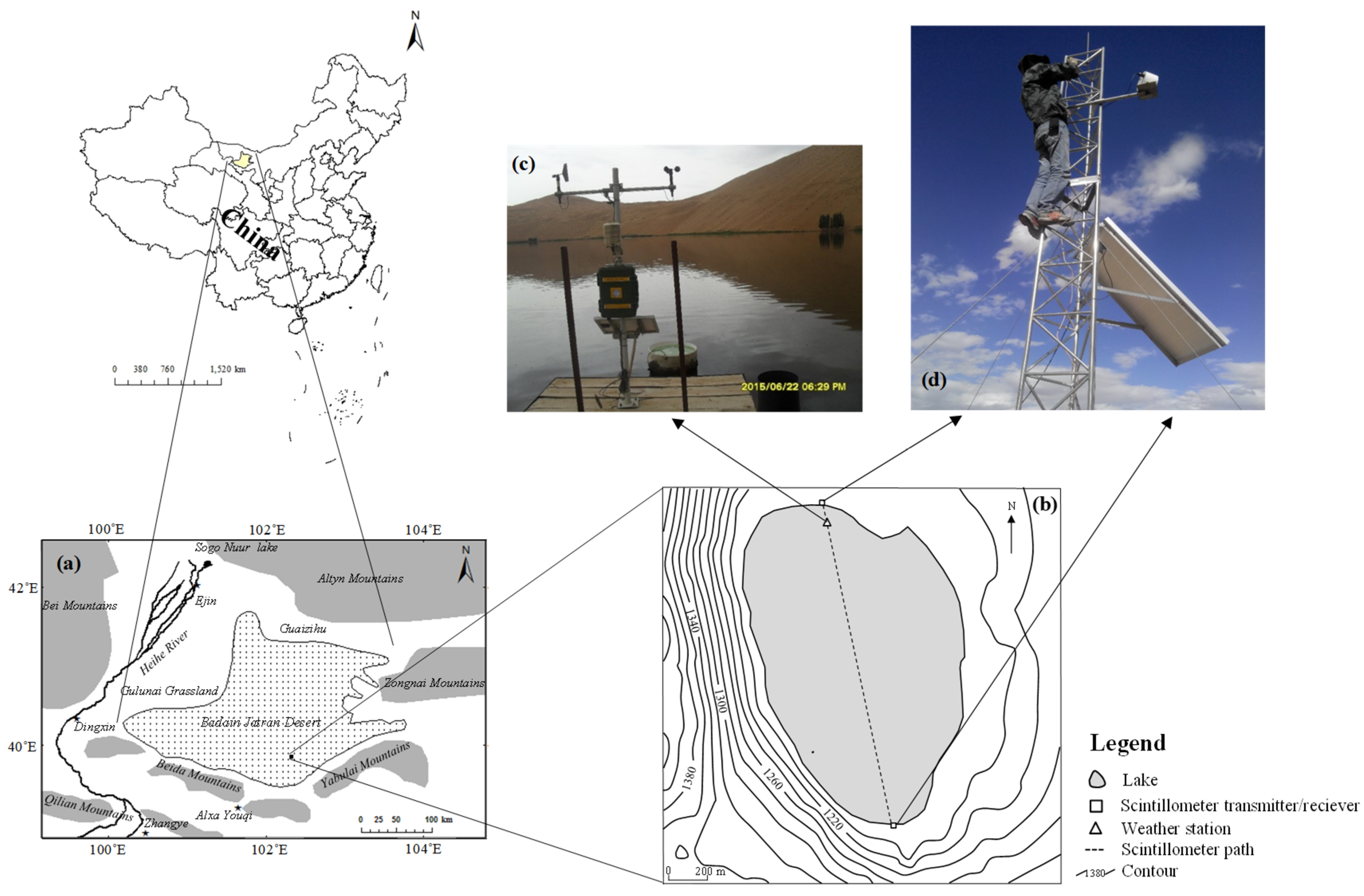
The Badain Jaran Desert (BJD) (39°20′–41°30′ N, 100°01′–103°10′ E) is located in the western Alxa Plateau, Inner Mongolia, China (Figure 1). It is the second-largest desert in China, with a total area of 4.9 × 10⁴ km² [27]. To the north, east, south, and southwest, the BJD is surrounded by mountains. The northwest of the BJD is Gurinai grassland lying in the downstream of the Heihe River. In the desert hinterland, numerous sand dunes and sandhills exist, covering as much as 60% of the desert. The heights of these sand dunes and sandhills can be up to 500 m with an average value ranging from 200–300 m. The average annual precipitation in the northwest is less than that in the southeast. The spatial distribution pattern of potential evaporation is just the opposite. Groundwater generally flows from south to north and from east to west with a hydraulic gradient of 0.8‰–7.9‰, which is consistent with the dominant slopes of desert topography.

Although in an arid climate, plenty of lakes exist in the BJD. However, most of them are smaller than 0.2 km² and shallower than 2 m. More than 65% of the lakes are saline lakes (i.e., total dissolved solids (TDS) >35 g L⁻¹) with salinity varying from 1 to 400 g L⁻¹. In this study, we focus on the second largest saline lake, the Sumu Barun Jaran. It has an area of 1.24 km² and a maximum depth of 11.1 m [28,29,30].

2.2. Calculation Procedure

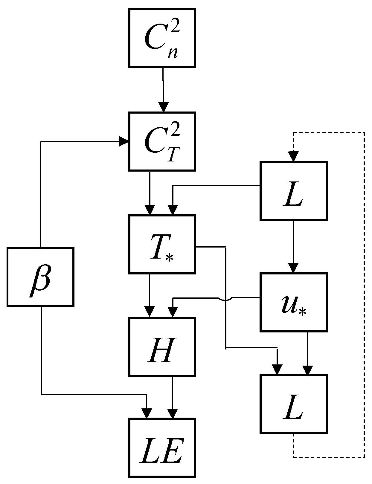
Utilizing the Monin–Obukhov similarity theory (MOST) [17] and site-specific meteorological data, the structure parameter of the refractive index ($C_n^2$) measured by scintillometer can be used to estimate the sensible heat flux, latent heat flux, and evaporation. The calculation procedure is shown in Figure 2.

Due to the fluctuations of temperature, humidity, and pressure in the atmosphere, the signal emitted by the transmitter may be disturbed by the turbulent atmosphere [31]. According to Wang et al. [32], $C_n^2$ can be expressed as

$$C_n^2=1.12{\sigma }_{\ln I}^2{D}^{7/3}{R}^{-3}$$

(2)

where D is the aperture diameter, R is the optical distance between the transmitter and the receiver, ${\sigma }_{\ln I}^2$ is the turbulent signal.

According to Hill et al. [33], $C_n^2$ can be used to obtain structure parameters of temperature ($C_T^2$), humidity ($C_Q^2$), and a covariant term ($C_{TQ}^2$). $C_T^2$ represents the air temperature fluctuation and can be obtained using the following equation [34]:

$$C_T^2=C_n^2{(\frac{T_a^2}{-0.78\times {10}^{-6}P})}^2{(1+\frac{0.03}{\beta })}^{-2}$$

(3)

where P is the atmospheric pressure, T_a is the absolute air temperature.

Based on the Monin–Obukhov similarity theory, the temperature scale ($T_{\ast }$) can be obtained as [35]

$$T_{\ast }{}^2=\frac{C_T^2{(z_s-d)}^{2/3}}{f_T(z_s/L)}$$

(4)

where z_s represents the scintillometer path height, d is the displacement height (d = 0 for open water [36]), and L is the Obukhov length. The sign (positive or negative) of $T_{\ast }$ can be determined from the atmospheric stability. As we have net radiation data, the net radiation method is used to determine the atmospheric stability, in which the net radiation >10 W m⁻² is considered as atmospheric instability [37]. The universal stability function f_T (z_s/L) proposed by Andreas [38] for unstable conditions is

$$f_T(z_s/L)=4.9{\left[1-6.1(\frac{z_s-d}{L})\right]}^{-2/3}$$

(5)

and for stable conditions is

$$f_T(z_s/L)=4.9\left[1+2.2{(\frac{z_s-d}{L})}^{2/3}\right]$$

(6)

The Obukhov length (L) can be estimated within an iterative approach, as follows:

$$L=\frac{u_{\ast }^2{T}_a}{gk{T}_{\ast }}$$

(7)

where g is gravitational acceleration, k is the von Karman constant, and $u_{\ast }$ is the friction velocity. Note that $u_{\ast }$ can be calculated by the standard flux profile relationship [39]:

$$u_{\ast }=\frac{ku}{\ln (\frac{z_u-d}{z_0})-{\phi }_m(\frac{z_u-d}{L})+{\phi }_m(\frac{z_0}{L})}$$

(8)

where u is the wind speed at the measurement height (z_u), and z₀ is the roughness length. In this study, we considered the fluctuations of the lake level and set the value of z₀ to be 0.0002 m, which is equal to the experiential value of sea. ${\phi }_m$ is a universal stability function of (z − d)/L [40]. For unstable conditions, it is calculated as

$${\phi }_m=2\ln \left[\frac{1+x}{2}\right]+\ln \left[\frac{1+x^2}{2}\right]-2\arctan (x)+\frac{\pi }{2} (L<0)$$

(9)

with

$$x={\left(1-\frac{16z}{L}\right)}^{1/4}$$

(10)

for stable conditions, it is calculated as

$${\phi }_m\left(\frac{z}{L}\right)=-5\frac{z}{L} (L>0)$$

(11)

Then we can calculate the value of H as follows,

$$H=-\rho c_p{T}_{\ast }{u}_{\ast }$$

(12)

where ρ is the density of air, c_p is the specific heat of air at a constant pressure.

The calculation procedure is an iterative process shown in Figure 2. We should specify the starting value of L before calculation, and the initial value of H can be subsequently calculated. Then a new value of L can be estimated, which is fed back via the iterative process to recalculate H. The procedure keeps running until the solution is stable. Once the value of H is obtained, the next step is to calculate the latent heat flux.

In this study, the classical method is applied to calculate the value of β using meteorological data over open water bodies. Specifically, if we assume that the turbulent transfer coefficients of heat and water vapor are equal above a water body, we can specify β on the basis of measurements of water temperature at the surface (T_w) and air temperature (T_a) as follows [41]:

$$\beta =\gamma \frac{T_s-T_a}{e_s^{\ast }-e_a}$$

(13)

where γ is the psychrometric constant, T_s is the water temperature at the surface, e_s^* is the surface water vapor pressure, e_a is the vapor pressure in the air, and the symbol of ^* denotes the state of saturation.

2.3. Field Data

As the measurement scale (200 m–10 km) of the large-aperture scintillometer matches well with the grid-scale of the satellite remote sensing, in recent years, it has become more and more popular to used to estimate heat fluxes and evaporation. Generally, the large-aperture scintillometer is observed synchronously with the eddy covariance system for comparing evaporation to test the results. As the evaporation of a lake can be measured directly by an evaporation pan and estimated by a simple aerodynamic model, it also can be used to verify the reliability of the large-aperture scintillometer.

A large-aperture scintillometer (LAS-BLS450, Scintec AG, Rottenburg, Germany) was installed on both sides of the Sumu Barun Jaran Lake. This equipment was mainly made up of two parts: a transmitter (39°47′44.30″ N, 102°25′19.93″ E) and a receiver (39°46′51.55″ N, 102°25′25.15″ E) with 150 mm aperture. The transmitted path length of the optical wave signal was 1801 m. The near-infrared pulse spectrum emitted by the transmitter was 880 nm, and the range of the structure parameter of the refractive index of air was from 10⁻¹⁷ to 10⁻¹⁰ m^−2/3. The modulation frequency of the scintillometer was 1750 Hz with an averaging period of 30 minutes.

An automatic weather station (AR5) manufactured by AVALON (Figure 1c) was installed on a wooden bridge in the Sumu Barun Jaran Lake for real-time recording of air temperature (TA), air relative humidity (RH), wind direction (WD), atmospheric pressure (AP), net radiation (R_n) and wind speed (WS) with an interval of 30 min. The top of the bracket was the anemometer (AV-30WS), the wind vane (AV-30WD) (the height of 202 cm from the bridge), and the net radiometer (AV-71NR) (185 cm distance to the bridge), respectively. A humidity sensor (AV-10TH) was installed at the height of 140 cm, under which is the data acquisition system (RR1016). At a distance of 135 cm from the bracket in the lake, an E601 evaporation pan was fixed with a conical steel frame. The evaporation pan was regularly filled with lake water, in which a CTD (conductance, temperature, and depth)-diver sensor (DI 271) with high precision (±2%) manufactured by Schlumberger Water Services was equipped for monitoring water level change automatically to calculate the evaporation. The temperature sensors (AV-10T) with high precision (±0.2 °C) were installed at the depths of 10 and 20 cm to measure water temperature (TS). Based on a survey of the lake water temperature at the surface and the depth-dependent temperature in the Sumu Barun Jaran lake, Chen et al. [42] found that shallow surface water within 6 m of the lake is driven by wind and solar radiation. The lake water temperature in the shallow surface layer tends to be evenly mixed, and vertical temperature gradient is small. The shallower the depth of the lake water, the closer its temperature is to the surface temperature of the lake water. Thus, it is reasonable to use the temperature at 10 cm depth to replace the water temperature at the lake surface. A self-recording pluviometer (AV-3665R) with a height of 73 cm from the bridge, a length of 22 cm and an outside diameter of 20 cm was equipped near the bracket. All data were collected by the data acquisition system.

Meteorological and scintillometer’s data from 12:00 on 26 October 2012 to 20:00 on 9 March 2013, from 8:00 on 10 May 2013 to 18:00 on 5 August 2013, and from 8:00 on 21 June 2014 to 20:00 on 26 March 2015 with the interval of 30 min in the daytime were collected in this study. 8:00 to 20:00 is defined as daytime, and the rest is defined as nighttime.

According to Wang et al. [43], the upper limit of the refractive index of air can be estimated using

$$C_n^2=0.193L_s{}^{-8/3}{\lambda }^{1/3}{D}^{5/3}$$

(14)

where L_s is the transmitted path length of the optical wave signal (1801 m), λ is the emitted wavelength of the electromagnetic wave (8.8 × 10⁻⁷ m), and D is the aperture of the scintillometer (0.15 m). Thus, the upper limit of the refractive index of air in the Sumu Barun Jaran is 1.63 × 10⁻¹³ m^−2/3, and data larger than the limit were removed.

3. Results

3.1. Reliability Analysis

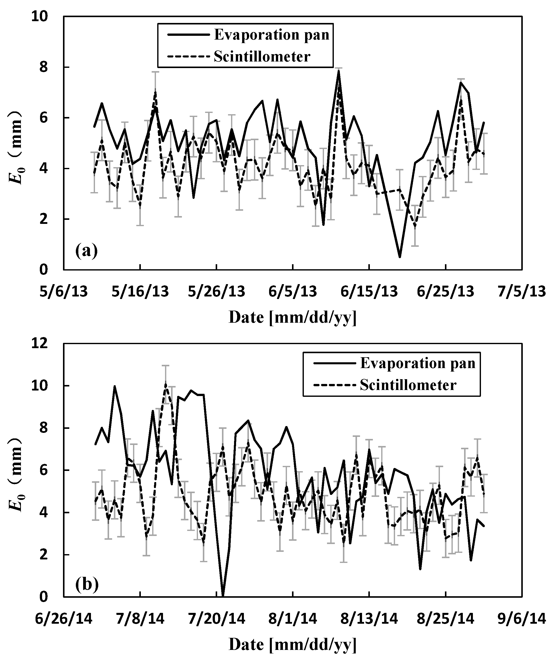
To valid the reliability of scintillometer in the estimation of evaporation for water bodies, we compared its results with E601 evaporation pan measurements. Due to the limited observation data of the evaporation pan, periods of 52 days from May 10 to 30 June 2013 and of 62 days from 1 July to 31 August 2014 were chosen to test the reliability of the scintillometer. The results are shown in Figure 3. The average daily evaporation measured by the evaporation pan and estimated by the scintillometer was 5.18 and 4.20 mm from May to June, and 5.89 and 4.90 mm from July to August, respectively. Fluctuations and magnitudes of daily evaporations calculated by the scintillometer were similar to those measured by the evaporation pan. Note that, in general, the results measured by the evaporation are larger than those estimated by the scintillometer. This could be ascribed to the different spatial scale observed by the two instruments.

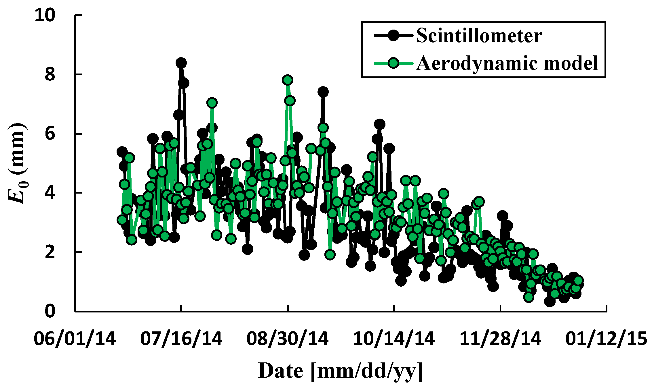
We also compare the results of the scintillometer with a simple aerodynamic model applied over open water bodies proposed by Mcjannet et al. [44]. Here, a long period from 21 June to 31 December 2014 was used to test the reliability of the scintillometer. For the aerodynamic model, it could be expressed as

$$E_0=(2.36+1.67\times WS)\times A^{-0.05}\times (e_s-e_a)$$

(15)

where A is the area of open water bodies (A = 1.24 × 10⁶ m²), e_s is the surface (10 cm) water vapor pressure, and e_a is the vapor pressure in the air. The results are shown in Figure 4. The daily evaporation estimated by the scintillometer ranges from 0.34 to 8.38 mm with an average value of 2.99 mm. The results calculated by the aerodynamic model vary between 0.49 and 7.81 mm with an average value of 3.32 mm. In comparison, the result estimated by the scintillometer is slightly higher and fluctuate with a larger amplitude. However, they show similar variation patterns. Therefore, we are confident that the scintillometer associated with the classical method is successfully applied to the Sumu Barun Jaran.

3.2. Flux Evaluation in Different Seasons with Water Temperature at Different Depths

Water temperature at the surface is a key parameter to estimate the heat fluxes and evaporation over open water bodies by using the classical method in the scintillometer procedure. The results in Section 3.1 demonstrate that water temperature at 10 cm depth can be used to replace the water temperature at the lake surface in the scintillometer procedure. Here, we will further investigate the seasonal changes in the heat flux evaluation by using water temperature at different depths (i.e., 10 and 20 cm). Note that the cold seasons and hot seasons are defined from November to February, and May to August, respectively.

3.2.1. Half-hour Time Scale

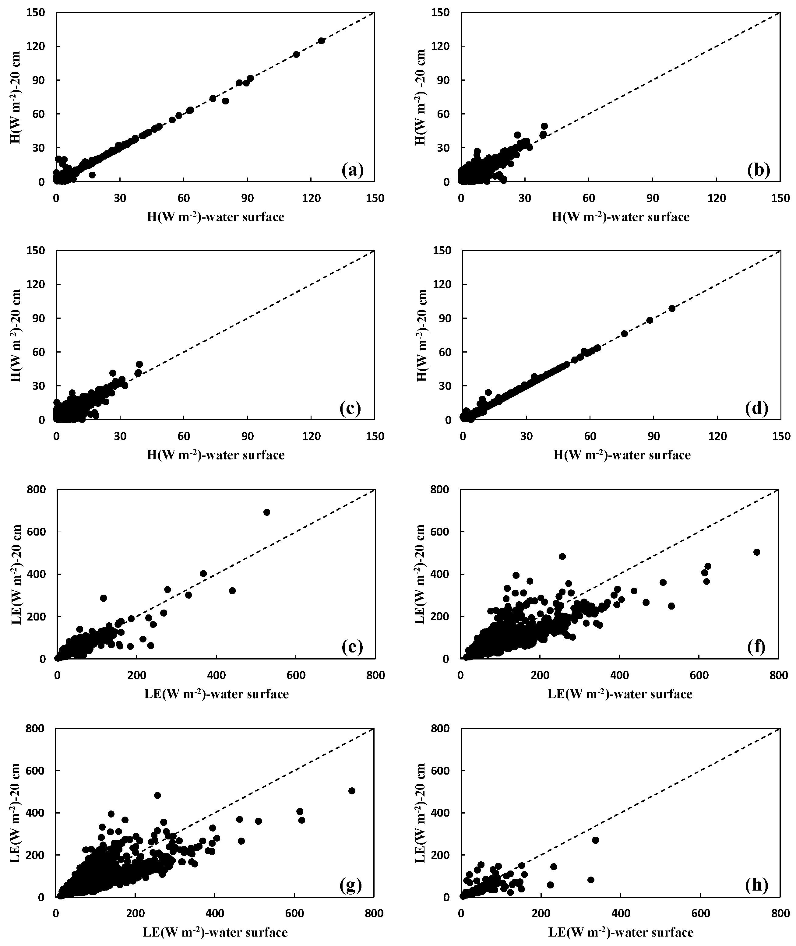
The results at the half-hour time scale are shown in Figure 5. Using water temperature at the lake surface (10 cm), the average values of H and LE are 10.83 and 32.37 W m⁻², respectively, in January and February, and 7.00 and 121.17 W m⁻² in May and June, 6.75 and 119.26 W m⁻² in July and August, and 14.77 and 30.65 W m⁻² in November and December. From cold to hot seasons, the average value of H decreases by 46%, and the average value of LE increases by 2.8 times.

Using water temperature at 20 cm depth, on average, the values of H and LE are 10.90 and 32.12 W m⁻², respectively, in January and February, 8.42 and 95.27 W m⁻² in May and June, 8.09 and 95.81 W m⁻² in July and August, and 14.91 and 27.74 W m⁻² in November and December. In cold seasons, the average value of H is 36% larger than that in hot seasons, and that of LE increases by approximately 2.2 times.

Therefore, the values of H were barely affected, and the average value of LE (E₀) using water temperature at 20 cm depth is 0.8%–9.5% smaller than that using water temperature at the surface. In hot seasons, compared with the results estimated by water temperature at the surface, the average value of H increased by 20%–30%, and that of LE (E₀) decreased by approximately 20% at 20 cm depth. Compared with the results using water temperature at the surface, the values of H and LE have greater fluctuations in hot seasons than those in cold seasons.

3.2.2. Daily Time Scale

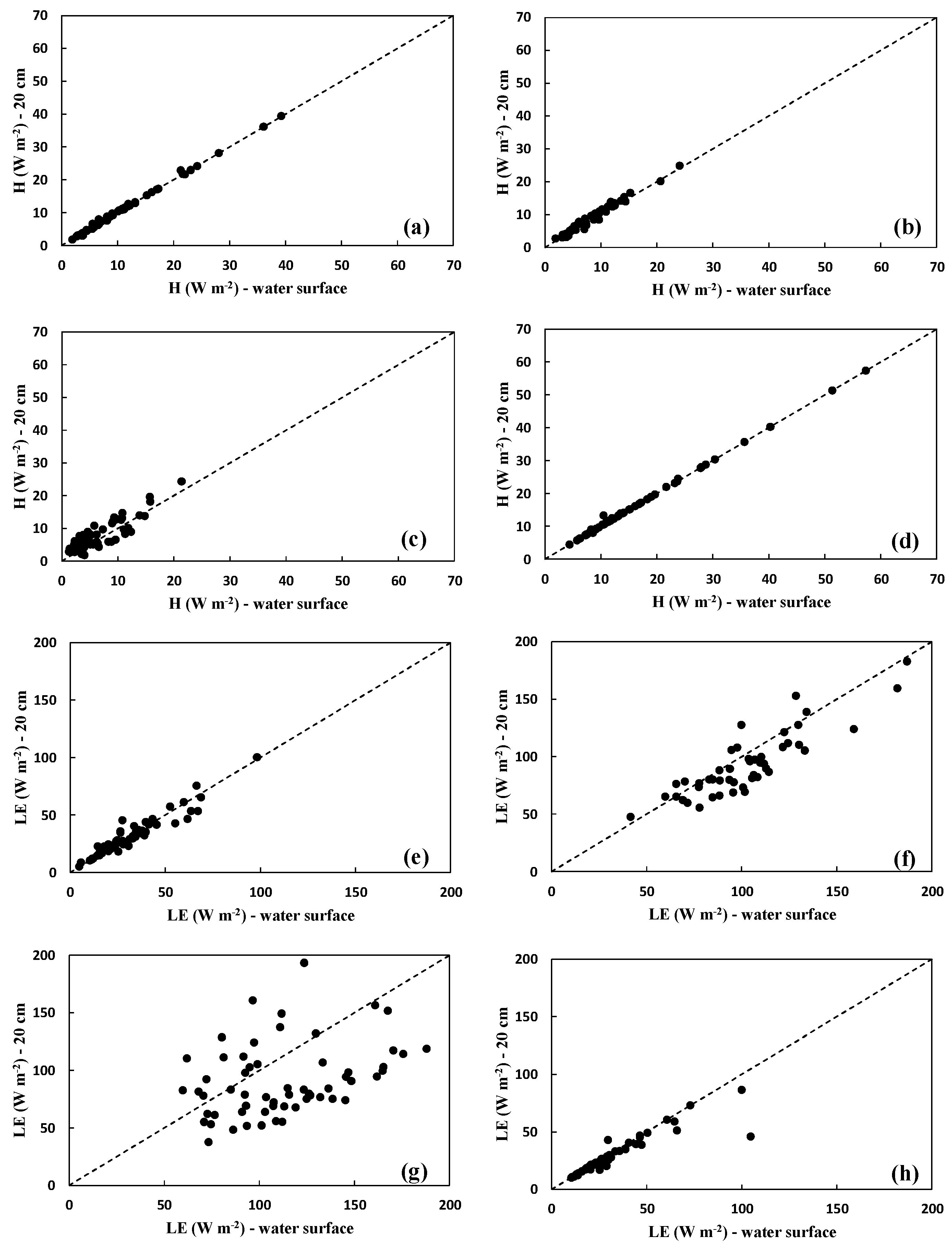
The results at the daily time scale are shown in Figure 6. Using water temperature at the lake surface (10 cm), the average values of H and LE are 11.04 and 31.56 W m⁻² in January and February, 8.34 and 102.44 W m⁻² in May and June, 6.70 and 116.63 W m⁻² in July and August, and 15.37 and 30.28 W m⁻² in November and December, respectively. From cold to hot seasons, on average, the value of H decreases by 43%, and the value of LE increases by about 2.5 times.

Using water temperature at 20 cm depth, the averages value of H and LE are 11.10 and 31.49 W m⁻² in January and February, 8.86 and 92.63 W m⁻² in May and June, 7.93 and 95.33 W m⁻² in July and August, and 15.49 and 27.70 W m⁻² in November and December, respectively. In cold seasons, on average, the value of H is 37% larger than that in hot seasons, and that of LE increases by approximately 2.2 times.

On the whole, in cold seasons, the values of H were almost unchanged. The daily average value of LE using water temperature at 20 cm depth is 0.2%–8.5% smaller than that by water temperature at the surface, and the root mean square error (RMSE) is 7.03 W m⁻². In hot seasons, compared with the results using water temperature at the surface, the average value of H increased by 6.2%–18.3% (RMSE = 1.70 W m⁻²), and that of LE decreased by 9.6%–18.3% (RMSE = 30.38 W m⁻²) at 20 cm depth. Compared with the results using water temperature at the surface, the values of H and LE using water temperature at 20 cm depth have greater fluctuations in hot seasons than those in cold seasons.

4. Discussion

4.1. Surface Roughness Length

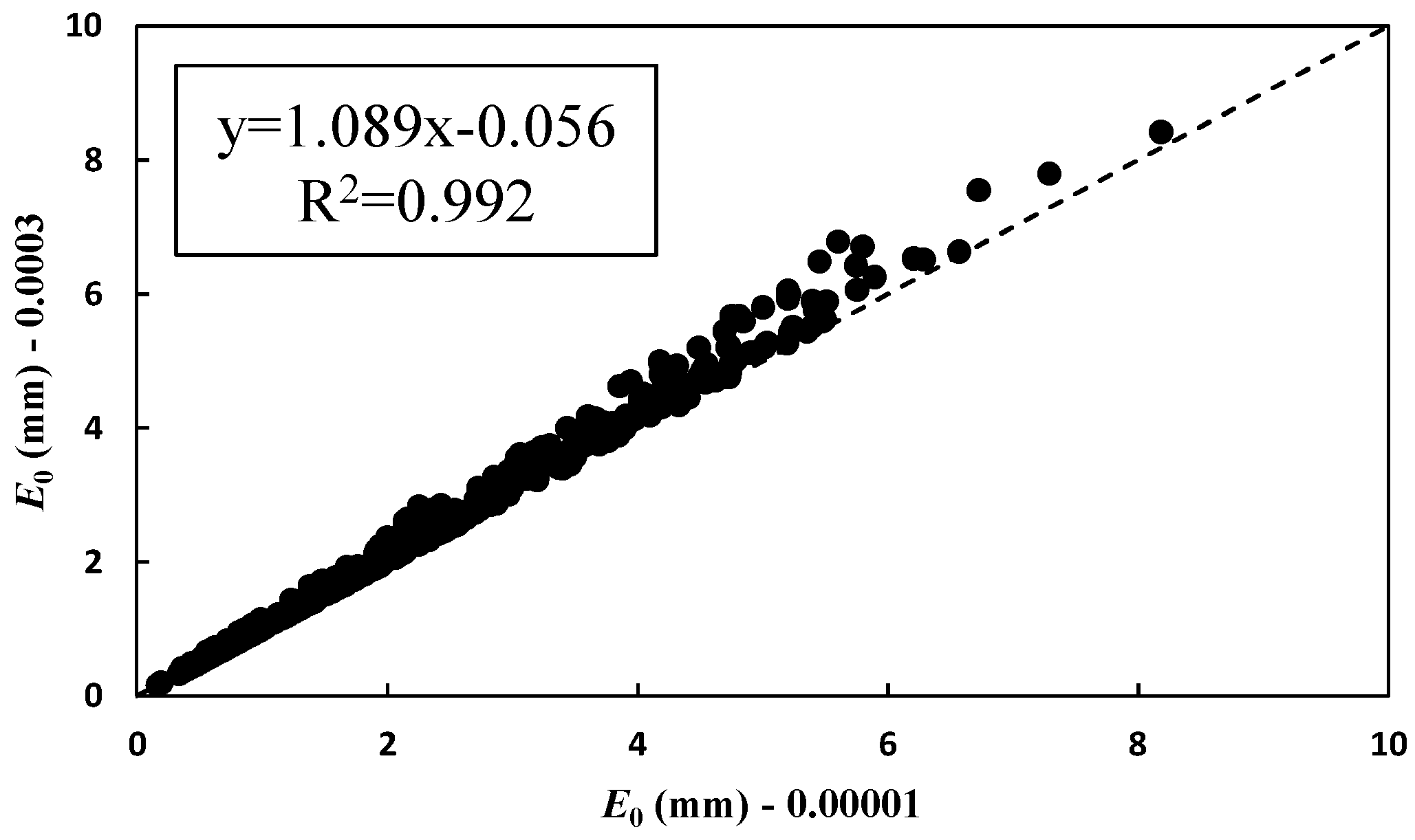
According to Section 2.2, evaporation is affected by the surface roughness length (z₀) to a certain degree. In the literature, Mcjannet et al. [6] pointed out that the value of z₀ has a limited range of variation, and that 90% of estimated values fall in the range from 9 × 10⁻⁵ to 1.7 × 10⁻⁴ m at Logan’s Dam in southeast Queensland, Australia. The surface roughness length of the sea obtained by Wieringa [45] is 0.0002 m. Based on these, we conducted sensitivity analyses of z₀ ranging from 0.00001 to 0.003 m to evaporation (Figure 7). The results show that, on average, the evaporation with a z₀ value of 0.0003 m is only 6% (RMSE = 0.24 mm) higher than that with a z₀ value of 0.00001 m. As z₀ has little effect on the evaporation, we specify z₀ with a value of 0.0002 m in this study.

4.2. Inconsistent Evaporations by Evaporation Pan, Eddy Covariance and Scintillometer

Although the results of the scintillometer are considered to be reliable by comparing the results with the evaporation pan data and the aerodynamic model, a comparison with the results of the eddy covariance system reported by previous studies is also used to further test its feasibility. According to the eddy covariance system installed on a small island far from the shore of the Yindeertu Lake, a lake similar to the Sumu Jaran Lake in the BJD, Hu et al. [46] and Su et al. [47] found that the daily evaporation of the lake varied from 0 to 12.21 mm with an average of 4.00 mm. The trend of fluctuation with time is consistent with the data of the evaporation pan. As the TDS of the Sumu Jaran Lake is larger, its evaporation should be smaller than that of the Yindeertu Lake. In this study, the daily evaporation estimated by the scintillometer ranged from 0 to 14.39 mm, which is generally consistent with the result given by the eddy covariance system.

The evaporation estimated by the scintillometer, eddy covariance, and evaporation pan is of the same magnitude and of the consistent fluctuation trend, but they are not completely the same. For example, the evaporation calculated by scintillometer is less than that observed from the evaporation pan. The measurement scales of evaporation pan (E601), eddy covariance, and scintillometer are several meters, dozens to hundreds of meters, and hundreds of meters to kilometers, respectively. Thus, the main reason for the inconsistency may be that the three instruments estimate the evaporation at different spatial scales.

4.3. Seasonal Differences in Flux Evaluation with Water Temperature at Different Depths

According to the results in Section 3.2, when using shallow water temperature at 10 and 20 cm depths instead of water temperature at the surface, seasonal differences in flux evaluation exist. In summary, in cold seasons, the heat fluxes (H and LE) are less affected by water temperature at different depths, while in the hot seasons, the fluxes are more affected. The reason may be that the use of subsurface water temperature measurements raises errors in summer, as the water will be more stratified, whereas in winter the lake upper layer will be better mixed. In general, temperature stratification of lake water is related to solar radiation, air temperature, wind speed, water density, water quality, and topography [48,49,50]. For example, the solar radiation intensity in the vertical direction of the water body is continuously attenuated, causing the solar radiation absorbed to decrease layer by layer. The water temperature at the surface increases and the water body at the bottom layer is not heated. Thus, the temperature of the bottom water layer changes little, and water temperature stratification occurs. The stronger the solar radiation, the more likely it is to cause water temperature stratification. As the temperature change of lake water is very complicated and subtle, due to limited data at hand, it should be studied in the future.

5. Conclusions

Scintillometers are more and more appreciated due to their ability to estimate sensible (H) and latent (LE) heat fluxes accurately over scales of hundreds to thousands of meters. However, studies regarding the use of scintillometers to estimate the evaporative processes over open water bodies are rarely found. In this study, a scintillometer was installed on both sides of the shore over the Sumu Barun Jaran Lake in the Badain Jaran Desert to obtain sensible and latent heat fluxes and to further estimate evaporation. Compared with the evaporation pan, aerodynamic model, and eddy covariance system, the results are plausible.

Water temperature at 10 and 20 cm depths were further used to replace the water temperature at the lake surface to analyze the seasonal changes in the flux evaluation at half-hour and daily time scales, respectively. The results show that water temperature at 10 cm depth can be approximately used to estimate heat fluxes in the scintillometer procedure. Moreover, the heat fluxes are less affected by the water temperature at different depths in cold seasons but are more affected in hot seasons. The reason of seasonal differences in flux evaluation may be that the lake water is more stratified in summer, and more mixed in winter.

This study helps the understanding of lake-water evaporation in the Badain Jaran Desert and the uncertainties in measurements by large-aperture scintillometers in lake and reservoir environments.

References

- Kustas, W.P. Estimates of evapotranspiration with a one-layer and two-layer model of heat transfer over partial canopy cover. J. Appl. Meteorol. 1990, 29, 704–715. [Google Scholar] [CrossRef]
- Ortega-Farias, S.O.; Cuenca, R.H.; English, M. Hourly grass evapotranspiration in modified maritime environment. J. Irrig. Drain. Eng. 1955, 121. [Google Scholar] [CrossRef]
- Bou-Zeid, E. Climate change and water resources in Lebanon and the Middle East. J. Water Resour. Plan. Manag. 2002, 128, 343–355. [Google Scholar] [CrossRef] [Green Version]
- Vercauteren, N.; Bou-Zeid, E.; Huwald, H.; Parlange, M.B.; Brutsaert, W. Estimation of wet surface evaporation from sensible heat flux measurements. Water Resour. Res. 2009, 45, W06424. [Google Scholar] [CrossRef] [Green Version]
- Mcjannet, D.L.; Cook, F.J.; McGloin, R.P.; McGowan, H.A.; Burn, S. Estimation of evaporation and sensible heat flux from open water using a large aperture scintillometer. Water Resour. Res. 2011, 47, W05545. [Google Scholar] [CrossRef] [Green Version]
- Mcgloin, R.; Mcgowan, H.; Mcjannet, D.; Cook, F.; Sogachev, A.; Burn, S. Quantification of surface energy fluxes from a small water body using scintillometry and eddy covariance. Water Resour. Res. 2014, 50, 494–513. [Google Scholar] [CrossRef] [Green Version]
- Han, P.F.; Wang, X.S.; Istanbulluoglu, E. A null-parameter formula of storage-evapotranspiration relationship at catchment scale and its application for a new hydrological model. J. Geophys. Res. Atmos. 2018, 123, 2082–2097. [Google Scholar] [CrossRef]
- Lowe, L.D.; Webb, J.A.; Nathan, R.J.; Etchells, T.; Malano, H.M. Evaporation from water supply reservoirs: An assessment of uncertainty. J. Hydrol. 2009, 376, 261–274. [Google Scholar] [CrossRef]
- Ikebuchi, S.; Seki, M.; Ohtoh, A. Evaporation from Lake-Biwa. J. Hydrol. 1988, 102, 427–449. [Google Scholar] [CrossRef]
- Blanken, P.D.; Rouse, W.R.; Culf, A.D.; Spence, C.; Boudreau, L.D.; Jasper, J.N.; Kochtubajda, B.; Schertzer, W.M.; Marsh, P.; Verseghy, D. Eddy covariance measurements of evaporation from Great Slave Lake, Northwest Territories, Canada. Water Resour. Res. 2000, 36, 1069–1077. [Google Scholar] [CrossRef]
- Liu, H.; Zhang, Y.; Liu, S.; Jiang, H.; Sheng, L.; Williams, Q.L. Eddy covariance measurements of surface energy budget and evaporation in a cool season over southern open water in Mississippi. J. Geophys. Res. 2009, 114, D04110. [Google Scholar] [CrossRef]
- Nordbo, A.; Launiainen, S.; Mammarella, I.; Lepparanta, M.; Huotari, J.; Ojala, A.; Vesala, T. Long-term energy flux measurements and energy balance over a small boreal lake using eddy covariance technique. J. Geophys. Res. 2011, 116, D02119. [Google Scholar] [CrossRef]
- Guyot, A.; Cohard, J.M.; Anquetin, S.; Galle, S.; Lloyd, C.R. Combined analysis of energy and water balances to estimate latent heat flux of a sudanian small catchment. J. Hydrol. 2009, 375, 227–240. [Google Scholar] [CrossRef]
- Savage, M.J. Estimation of evaporation using a dual-beam surface layer scintillometer and component energy balance measurements. Agric. For. Meteorol. 2009, 149, 501–517. [Google Scholar] [CrossRef]
- Bouin, M.N.; Legain, D.; Traulle, O.; Belamari, S.; Caniaux, G.; Fiandrino, A.; Lagarde, F.; Barrie, J.; Moulin, E.; Bouhours, G. Using scintillometry to estimate sensible heat fluxes over water: First insights. Bound. Layer Meteorol. 2012, 143, 451–480. [Google Scholar] [CrossRef] [Green Version]
- Mcjannet, D.; Cook, F.; Mcgloin, R.; Mcgowan, H.; Burn, S.; Sherman, B. Long-term energy flux measurements over an irrigation water storage using scintillometry. Agric. For. Meteorol. 2013, 168, 93–107. [Google Scholar] [CrossRef]
- Monin, A.; Obukhov, A. Basic laws of turbulent mixing in the surface layer of the atmosphere. Contrib. Geophys. Inst. Acad. Sci. USSR 1954, 151, 163–187. [Google Scholar]
- Solignac, P.A.; Brut, A.; Selves, J.L.; Beteille, J.P.; Gastellu-Etchegorry, J.P.; Keravec, P.; Beziat, P.; Ceschia, E. Uncertainty analysis of computational methods for deriving sensible heat flux values from scintillometer measurements. Atmos. Meas. Tech. 2009, 2, 741–753. [Google Scholar] [CrossRef] [Green Version]
- Green, A.E.; Hayashi, Y. Use of the scintillometer technique over a rice paddy. Jpn. J. Agric. Meteorol. 1998, 54, 225–234. [Google Scholar] [CrossRef] [Green Version]
- Tanny, J.; Cohen, S.; Assouline, S.; Lange, F.; Grava, A.; Berger, D.; Teltch, B.; Parlange, M.B. Evaporation from a small water reservoir: Direct measurements and estimates. J. Hydrol. 2008, 351, 218–229. [Google Scholar] [CrossRef] [Green Version]
- Mcgowan, H.A.; Sturman, A.P.; Mackellar, M.C.; Weibe, A.H.; Neil, D.T. Measurements of the surface energy balance over a coral reef flat, Heron Island, southern Great Barrier Reef, Australia. J. Geophys. Res. 2010, 115, D19124. [Google Scholar] [CrossRef] [Green Version]
- Stannard, D.I.; Rosenberry, D.O. A comparison of short-term measurements of lake evaporation using eddy correlation and energy budget methods. J. Hydrol. 1991, 122, 15–22. [Google Scholar] [CrossRef]
- Chen, J.S.; Li, L.; Wang, J.Y.; Barry, D.A.; Sheng, X.F.; Gu, W.Z.; Zhao, X.; Chen, L. Water resources: Groundwater maintains dune landscape. Nature 2004, 432, 459–460. [Google Scholar] [CrossRef] [PubMed]
- Gates, J.; Edmunds, W.; Ma, J.; Scanlon, B. Estimating groundwater recharge in a cold desert environment in northern China using chloride. Hydrogeol. J. 2008, 16, 893–910. [Google Scholar] [CrossRef]
- Yang, X.P.; Ma, N.; Dong, J.F.; Zhu, B.; Xu, B.; Ma, Z.; Liu, J. Recharge to the inter-dune lakes and Holocene climatic changes in the Badain Jaran Desert, western China. Quat. Res. 2010, 73, 10–19. [Google Scholar] [CrossRef]
- Wang, X.S.; Hu, B.X.; Jin, X.M.; Hou, L.Z.; Qian, R.Y.; Wang, L.D. Interactions between groundwater and lakes in Badain Jaran Desert. Earth Sci. Front. 2014, 21, 91–99. (In Chinese) [Google Scholar] [CrossRef]
- Wang, T. Formation and evolution of Badain Jaran Sandy Desert, China. J. Desert Res. 1990, 10, 29–40. (In Chinese) [Google Scholar]
- Wang, X.S.; Zhou, Y. Investigating the mysteries of groundwater in the Badain Jaran Desert, China. Hydrogeol. J. 2018, 26, 1639–1655. [Google Scholar] [CrossRef]
- Wen, J.; Han, P.F.; Zhou, Z.; Wang, X.S. Lake level dynamics exploration using deep learning, artificial neural network, and multiple linear regression techniques. Environ. Earth Sci. 2019, 78. [Google Scholar] [CrossRef]
- Han, P.F.; Wang, X.S.; Bill, X.H.; Jiang, X.W.; Zhou, Y. Dynamic relationship between lake surface evaporation and meteorological factors in the Badain Jaran Desert. Arid Zone Res. 2018, 35, 1012–1020. (In Chinese) [Google Scholar] [CrossRef]
- Meijninger, W.M.L.; Green, A.E.; Hartogensis, O.K.; Kohsiek, W.; Hoedjes, J.C.B.; Zuurbier, R.M.; De Bruin, H.A.R. Determination of area-averaged water vapour fluxes with large aperture and radio wave scintillometers over a heterogeneous surface-Flevoland field experiment. Bound. Layer Meteorol. 2002, 105, 63–83. [Google Scholar] [CrossRef]
- Wang, T.; Ochs, G.R.; Clifford, S.F. A saturation-resistant optical scintillometer to measure C2n. J. Opt. Soc. Am. 1978, 68, 334–338. [Google Scholar] [CrossRef]
- Hill, R.J.; Clifford, S.F.; Lawrence, R.S. Refractive-index and absorption fluctuations in the infrared caused by temperature, humidity, and pressure fluctuations. J. Opt. Soc. Am. 1980, 70, 1192–1205. [Google Scholar] [CrossRef]
- Wesley, M.L. The combined effect of temperature and humidity fluctuations on refractive index. J. Appl. Meteorol. 1976, 15, 43–49. [Google Scholar] [CrossRef]
- Wyngaard, J.C.; Izumi, Y.; Collins, J.S.A. Behavior of the Refractive-Index-Structure Parameter near the Ground. J. Opt. Soc. Am. 1971, 61, 1646–1650. [Google Scholar] [CrossRef]
- Oke, T.R. Boundary Layer Climates. Earth-Sci. Rev. 1987, 28, 258–319. [Google Scholar] [CrossRef]
- Kohsiek, W.; Meijninger, W.M.L.; Debruin, H.A.R.; Beyrich, F. Saturation of the large aperture scintillometer. Bound. Layer Meteorol. 2006, 121, 111–126. [Google Scholar] [CrossRef]
- Andreas, E.L. Atmospheric stability from scintillation measurements. Appl. Opt. 1988, 27, 2241–2246. [Google Scholar] [CrossRef]
- Panofsky, H.; Dutton, J. Atmospheric Turbulence: Models and Methods for Engineering Applications; John Wiley: Hoboken, NJ, USA, 1984. [Google Scholar] [CrossRef]
- Businger, J.A.; Miyake, M.; Dyer, A.J.; Bradley, E.F. On the Direct Determination of the Turbulent Heat Flux Near the Ground. J. Appl. Meteorol. 1967, 6, 1025–1032. [Google Scholar] [CrossRef] [Green Version]
- Penman, H.L. Natural evaporation from open water, bare soil and grass. Proc. R. Soc. Lond. Ser. A 1948, 193, 120–145. [Google Scholar] [CrossRef] [Green Version]
- Chen, T.F.; Wang, X.S.; Bill, X.H.; Lu, H.T.; Gong, Y.P. Clines in salt lakes in the Badain Jaran Desert and their significances in indicating fresh groundwater discharge. J. Lake Sci. 2015, 27, 183–189. (In Chinese) [Google Scholar] [CrossRef]
- Wang, W.; Xu, Z.; Li, X.; Wang, J.; Zhang, Z. A Study of Applications of Large Aperture Scintillometer in the Heihe River Basin. Adv. Earth Sci. 2010, 25, 1208–1216. (In Chinese) [Google Scholar] [CrossRef]
- Mcjannet, D.L.; Webster, I.T.; Cook, F.J. An area-dependent wind function for estimating open water evaporation using land-based meteorological data. Environ. Model. Softw. 2012, 31, 76–83. [Google Scholar] [CrossRef]
- Wiernga, J. Representative roughness parameters for homogeneous terrain. Bound. Layer Meteorol. 1993, 63, 323–363. [Google Scholar] [CrossRef]
- Hu, W.; Wang, N.; Zhao, L.; Ning, K.; Zhang, X.; Sun, J. Water-heat exchange over a typical lake in Badain Jaran Desert, China. Prog. Geogr. 2015, 34, 1061–1071. (In Chinese) [Google Scholar] [CrossRef]
- Su, J.; Hu, W.; Wang, N.; Zhao, L.; An, R.; Ning, K.; Zhang, X. Eddy covariance measurements of water vapor and energy flux over a lake in the Badain Jaran Desert, China. J. Arid Land 2018, 10, 517–533. [Google Scholar] [CrossRef] [Green Version]
- Branco, B.F.; Torgersen, T. Predicting the onset of thermal stratification in shallow inland waterbodies. Aquat. Sci. 2009, 71, 65–79. [Google Scholar] [CrossRef]
- Magee, M.R.; Wu, C.H. Response of water temperatures and stratification to changing climate in three lakes with different morphometry. Hydrol. Earth Syst. Sci. 2017, 21, 6253–6274. [Google Scholar] [CrossRef] [Green Version]
- Bueche, T.; Vetter, M. Simulating water temperatures and stratification of a pre-alpine lake with a hydrodynamic model: Calibration and sensitivity analysis of climatic input parameters. Hydrol. Process. 2014, 28, 1450–1464. [Google Scholar] [CrossRef]
Figure 1.
Locations of the study area (a), Sumu Baran lake (b), weather station (c), and scintillometer (d).
Figure 2.
Schematic diagram of the calculation procedure to estimate heat fluxes by the scintillometer.
Figure 3.
Dynamic variations of the estimated evaporation by scintillometer with the water temperature at 10 cm depth and observed results from the evaporation pan at a daily time during 10 May 2013–30 June 2013 (a) and 1 July 2014–31 August 2014 (b).
Figure 4.
Dynamic variations of the estimated evaporation by the scintillometer with water temperature at 10cm depth and the aerodynamic model at the daily time scale during 21 June 2014–31 December 2014.
Figure 5.
Comparison of the results of H and LE estimated by the scintillometer using water temperature at the lake surface (10 cm) and using water temperature at 20 cm depth at the half-hour time scale in January and February 2013 (a,e), May and June 2013 (b,f), July and August 2014 (c,g), and November and December 2012 (d,h).
Figure 6.
Comparison of the results of H and LE by the scintillometer using lake-water surface temperature (10 cm) and using water temperature at 20 cm depth at the daily time scale in January and February 2013 (a,e), May and June 2013 (b,f), July and August 2014 (c,g), and November and December 2012 (d,h).
Figure 7.
The sensitivity of z0 with a range from 0.00001 to 0.003 m to evaporation.
© 2019 by the authors. Licensee MDPI, Basel, Switzerland. This article is an open access article distributed under the terms and conditions of the Creative Commons Attribution (CC BY) license (http://creativecommons.org/licenses/by/4.0/).
Share and Cite
MDPI and ACS Style
Han, P.-F.; Wang, X.-S.; Wang, J.-Z. Using Large-Aperture Scintillometer to Estimate Lake-Water Evaporation and Heat Fluxes in the Badain Jaran Desert, China. Water 2019, 11, 2575. https://doi.org/10.3390/w11122575
AMA Style
Han P-F, Wang X-S, Wang J-Z. Using Large-Aperture Scintillometer to Estimate Lake-Water Evaporation and Heat Fluxes in the Badain Jaran Desert, China. Water. 2019; 11(12):2575. https://doi.org/10.3390/w11122575
Chicago/Turabian StyleHan, Peng-Fei, Xu-Sheng Wang, and Jun-Zhi Wang. 2019. "Using Large-Aperture Scintillometer to Estimate Lake-Water Evaporation and Heat Fluxes in the Badain Jaran Desert, China" Water 11, no. 12: 2575. https://doi.org/10.3390/w11122575
Note that from the first issue of 2016, this journal uses article numbers instead of page numbers. See further details here.