Article

Green Water on A Fixed Structure Due to Incident Bores: Guidelines and Database for Model Validations Regarding Flow Evolution

by
Jassiel V. Hernández-Fontes
1,2,*,
Paulo de Tarso T. Esperança
2,
Juan F. Bárcenas Graniel
3,
Sergio H. Sphaier
2 and
Rodolfo Silva
1
1
II-UNAM, Instituto de Ingeniería, Universidad Nacional Autónoma de México, Edificio 17, Ciudad Universitaria, Mexico City 04510, Mexico
2
LabOceano (Laboratório de Tecnologia Oceânica), Programa de Engenharia Oceânica, COPPE/UFRJ, Universidade Federal do Rio de Janeiro, Parque Tecnológico do Rio, Rio de Janeiro 21941-907, Brazil
3
Departamento de Ciencias Básicas e Ingeniería, Universidad del Caribe, SM. 78, Manzana 1, Lote 1, Esq. Fraccionamiento Tabachines, Cancun 77528, Quintana Roo, Mexico
*
Author to whom correspondence should be addressed.
Water 2019, 11(12), 2584; https://doi.org/10.3390/w11122584
Submission received: 19 November 2019 / Revised: 3 December 2019 / Accepted: 3 December 2019 / Published: 7 December 2019
(This article belongs to the Special Issue Interaction between Waves and Maritime Structures)

Abstract

:
This paper presents a two-dimensional experimental study of the interaction of wet dam-break bores with a fixed structure, regarding the evolution of the incident flows and the resultant green water events on the deck. The study employs image-based techniques to analyse flow propagation from videos taken by high-speed cameras, considering five different shipping water cases. The features of small air-cavities formed in some green water events of the plunging-dam-break type were analysed. Then, the spatial and temporal distribution of water elevations of the incident bores and green water were investigated, providing a database to be used for model validations. Some guidelines for the selection of the freeboard exceedance, which is of relevance for green water simulations, were provided. Finally, the relationship between the incident bore and water-on-deck kinematics was discussed. The proposed study can be used as a reference for performing simplified and systematic analyses of green water in a different two-dimensional setup, giving high-resolution data that visually capture the flow patterns and allow model validations to be performed.

1. Introduction

Green water events, defined as compact masses of water shipping on the deck of marine structures [1], are phenomena of importance in applications involving the interaction of waves with fixed, moored, free-floating, or advancing devices. Detailed analyses of such events can help to improve the design of these structures.
The study of green water events has employed methodologies that are analytical [2,3,4], numerical [1,5,6], and experimental [7,8,9]. The latter methodology type is important since it can be used to validate analytical and numerical models. However, at the model scale, green water events occur in a short time and must be captured at adequate sampling rates to give sufficiently detailed information to validate the models.
Experiments on green water have been carried out using wave trains in wave flumes [1,7,10] and ocean basins [2,11]. Sometimes, these experiments take long periods of time, requiring a reduction in the sampling rates of sensors and cameras to capture enough details of the green water events generated. Recently, the need for more detailed investigations to better understand the types of green water events that impinge on structures has been noted in the literature [12]. It was seen as necessary to employ high-resolution tecniques in the study of green water patterns and their evolution over the deck. Some research that has treated these topics includes the works of [5,7]. They presented two-dimensional experimental studies of green water using regular wave trains, reporting several types of green water events. However, the water elevations of the incoming wave and green water were monitored by obstructive wave probes at very few positions [1], thus limiting a more detailed understanding of the water evolution along the deck.
Later on, Ryu et al. [10,13] also used a two-dimensional experimental setup to study green water, considering a broken incident wave. However, the focus of their works was the study of the wave kinematics by applying an image-based method, disregarding the identification of flow patterns and the evolution of water in terms of elevations.
In order to understand details of different types of green water events, Hernández-Fontes et al. [14,15] proposed an alternative approach to generate systematic experiments of green water in a controlled environment, investigating the resulting patterns. They used the wet dam-break method in a small rectangular tank (~1 m length) to generate incident bores, which produced isolated green water events on a fixed rectangular structure. The wet dam-break method considers the flow generated from the sudden interaction of a water volume located upstream of a vertical gate (initial water depth, h1) with a water volume located downstream of the gate (initial water depth, h0), taking into account that h1 is always higher than h0 ([16]). From a high-speed video, Hernández-Fontes et al. [14,15] presented snapshots and descriptions of events that had some resemblance with the dam-break (DB), plunging-dam-break (PDB), and hammer-fist (HF) types reported by [7]. In the DB, the flow flooding the deck resembles a dam-break type flow. In the PDB, a cavity forms at the beginning of the deck followed by a DB flow. In the HF-type, a block of water rises at the bow, forming a suspended arm that directly hits the deck.
The use of the wet dam-break approach to study the green water problem in a simplified way is a recent proposal [14,15]. However, the study of the physics and applications of such a method is not new. Early experimental research was performed by [17], who investigated the resulting flows based on their kinematic characteristics. Some years later, Stoker [16] established well-known analytical procedures to represent the physics of dry (h0 = 0, see also [18]) and wet (h0 > 0, h0 < h1) dam-break phenomena, considering infinite conditions in the flow propagation domains. Later, Nakagawa et al. [19] performed several experimental tests to characterize the flow resulting from the dry and wet dam-break cases in a 0.5 m wide and 30 m long wave flume, employing the Stoker approach to analyse the resulting flows. From their observations, they proposed three types of wet dam-break flow based on the h0/h1 ratio: A wave of uniform and progressive features with a breaking front, similar to a moving hydraulic jump (0 < h0/h1 ≤ 0.4); a wave resembling an undular bore of unstable dynamics with its front partially broken (0.4 < h0/h1 ≤ 0.56); and a wave similar to an undular bore with its front unbroken (0.56 ≤ h0/h1 < 1.0). Later on, in a flume 0.4 m wide and 15.24 m long, Stansby et al. [20] performed a numerical and experimental study, considering the ratios h0/h1 = 0.1 and 0.45 to investigate the initial stages of the wet dam-break problem. They reported that a mushroom-like jet is formed just after gate release, which interacts with the downstream, quiet water in a complex way, entraining air before a wave resembling a bore or a spilling breaker is developed. These findings were further confirmed numerically by [21]. Other studies have employed dam-break flows to study their interactions with structures located downstream. For example, Oertel and Bung [22], through experimental and numerical tests, evaluated the effects of a rectangular obstacle on the flow derived from the dry dam-beak case (h0 = 0, h1 > 0). Also, using numerical and experimental methods, Kocaman and Ozmen-Cagatay [23] investigated the impacts of wet dam-break waves on a vertical wall. More recently, Hernández-Fontes et al. [24,25] used the experimental wet dam-break approach to investigate green water problems, validating an analytical model for green water elevations and loading over the deck of a fixed structure, respectively.
The use of the wet dam-break method to investigate the green water problem on fixed structures can still be extended to explain in more detail the interaction of the incident flow with the structure and to increase the understanding of the physics of different green water patterns. This paper thus extends the experimental wet dam-break application of [14,15], described above, to investigate details of the interaction of bores with a fixed rectangular structure, using image-based analyses to study the flow evolution in time and space. The evolution of the incoming bores and the generated green water events, in terms of water elevations, are included in this research. As an alternative to previous two-dimensional green water studies that have been performed with other methods, such as regular waves, this paper offers an approach that allows some details in green water research to be investigated in a systematic and practical way. The main objectives are described as follows:
(a)
To analyse features of the air cavities formed at the beginning of the deck during the initial stages of some green water events that occur in the form of a plunging-dam-break.
(b)
To investigate the spatial and temporal evolution of the incident flow and the resultant water on deck of the structure, providing a database of time series of water elevations for all the study cases performed in this work, which can be employed by other authors to validate analytical or numerical models. The procedure followed to obtain these data can be very helpful to analyse green water elevations in other two-dimensional applications, which until now, have generally been measured at only a few positions, by obstructive wave probes.
(c)
To analyse the difference between selecting the freeboard exceedance at the bow or an upstream position, including the relationship existing between the freeboard exceedance and the incident bores. This parameter is of significant relevance in performing model implementations, then the approach followed here may be useful to evaluate adequate safety factors to predict the real amount of water on deck.
(d)
To verify the relationship between the kinematics of green water with that of the incident bore, including the influence of the presence of the structure.
These topics were investigated in a dam-break installation of approximately 2 m in length, considering the interaction of five different wet dam-break bores with a fixed rectangular structure located downstream. The bores were generated with a wet dam-break ratio of h0/h1 = 0.6 and five freeboards (0.006 m ≤ FB ≤ 0.042 m). Experiments with and without the fixed structure were performed. High-speed cameras and conductive wave probes were employed to monitor flow propagation. The videos were analysed with open-source image-based methods to extract water elevation measurements at several positions along the installation, allowing a detailed visualization of flow evolution in time and space.
The paper is organized as follows: Section 2 briefly presents the theoretical wet dam-break approach. The experimental methods are shown in Section 3 and the comparisons of a conventional technique with VWPs (virtual wave probes, as named by [26]) are shown in Section 4. Then, the incoming wave and green water results are presented in Section 5 and Section 6, respectively. Finally, Section 7 summarizes the main conclusions and future works.

2. The Theoretical Wet Dam-Break Approach

In the present experimental investigation, the isolated green water events were reproduced using the wet dam-break approach as the mechanism to generate the incident waves (i.e., bores). In this approach, a dam (gate) separates two sides of a horizontal tank of constant cross section at x = 0. Upstream and downstream of the dam, there is a volume of water with an initial water depth, h1 and h0, respectively. It is assumed that the tank extends to infinite in upstream and downstream directions, and that h1 is always higher than h0.
At the initial condition, the water at both sides of the dam is assumed as undisturbed (i.e., at rest position). Then, the gate is suddenly removed (t = 0). In this stage, the rapid formation of a wave in the form of a bore or a hydraulic jump [16] is expected in the downstream region, propagating with theoretical front velocity, U0, and elevation, h2, over the lower layer of water. These parameters were estimated from the graphical solution proposed by [16], verifying its applicability to the present experimental application. To apply this theoretical model, the effects of the finite length of the water reservoirs were neglected, assuming the infinite domains of propagation described by Stoker’s theory.

3. Experimental Methods

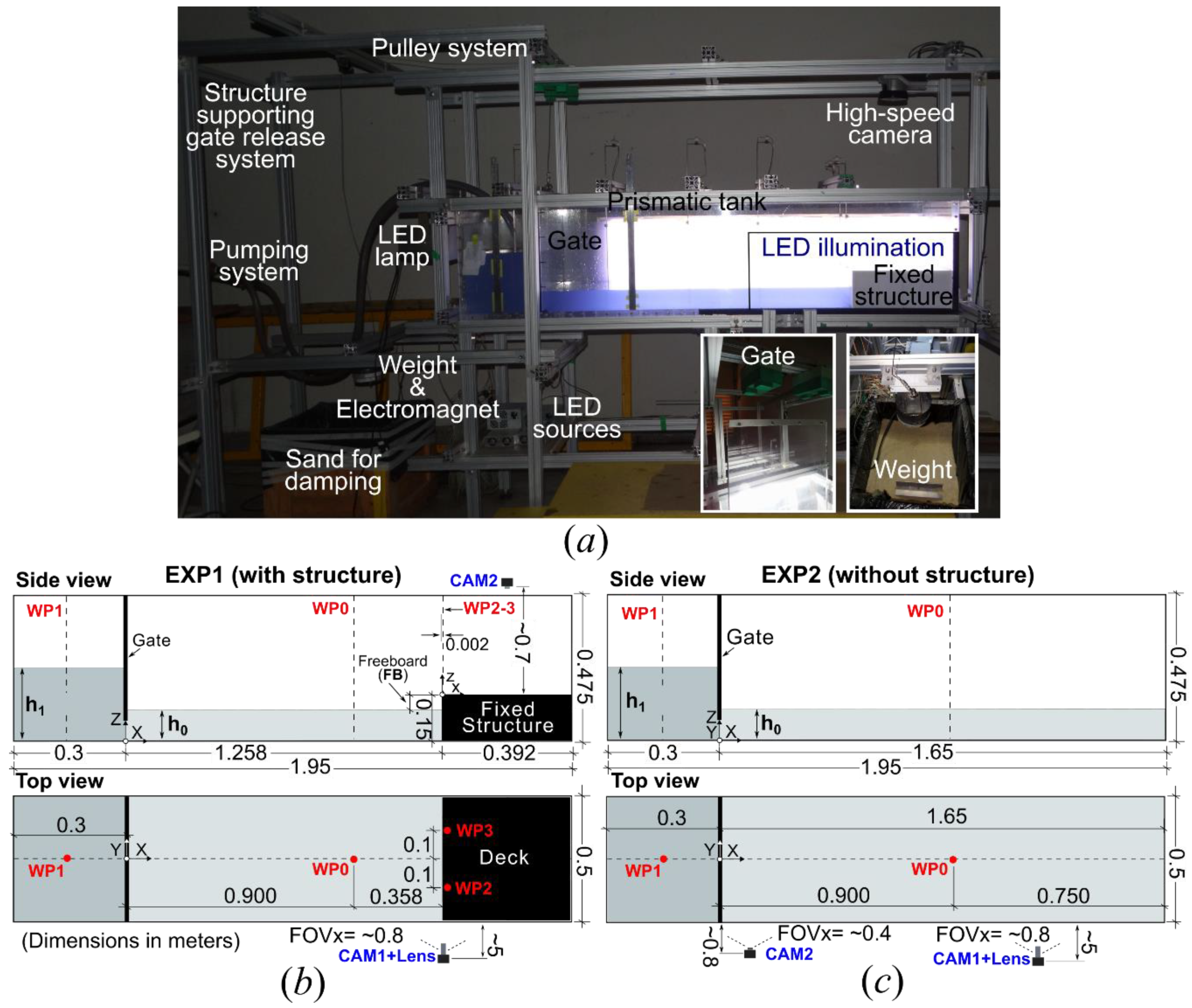
3.1. Experimental Set-Up

The wet dam-break experiments were carried out at the Ocean Technology Laboratory (LabOceano/COPPE) facilities of the Federal University of Rio de Janeiro, Brazil.
The general arrangement of the experiment can be seen in Figure 1a. A prismatic tank, made of polymethyl methacrylate (PMMA) plates, 25 mm thick, to reduce hydroelastic effects, was mounted on a structural arrangement. This tank had a fixed rectangular box installed inside, representing the deck of a coastal, naval, or offshore structure. At the left side of the tank, a vertical gate separating an upstream volume of water from a downstream volume can be observed. This was made from a PMMA plate, 15 mm thick. The gate was pulled upwards (dam-break action) by a release mechanism mounted in a vertical structure separated from the tank support. The release mechanism was formed by a 16 kgf weight, held by an electromagnet at the beginning of the experiments. When the trigger was activated (t = 0 s), the weight fell down and opened the gate by means of a pulley arrangement in the external structure.
In the present investigation, two types of experiments were carried out, considering the dam-break installation with (EXP1) and without (EXP2) the internal fixed structure. The main dimensions of the tank as well as the sensor positions for EXP1 and EXP2 are shown in Figure 1b,c, respectively.

3.2. Study Cases

In this work, five different cases of green water on a fixed structure were considered (C1–C5), as shown in Table 1. These were generated with the wet dam-break aspect ratio, h0/h1 = 0.6, and five different freeboards (FB, Figure 1b). The study case, C1, was employed as representative of the other cases for the main descriptions of the topics of the present work. However, all the cases were employed for comparison and discussion purposes.
The ratio h0/h1 = 0.6 was chosen to generate unbroken incident flows, as suggested by [19]. Hernández-Fontes et al. [14], obtained unbroken incident flows considering the same wet dam-break ratio, with a smaller tank than that of this study. In that work, such a ratio caused isolated green water events that generated small cavities at the beginning of the deck, which were also expected in the present study.
The aim was to generate unbroken incident flows in order to apply a two-dimensional image-based methodology for the investigation of flow evolution (Section 3.4). It is important to mention that the features of the resultant wet dam-break wave might change according to the experimental setup. Yeh et al. [27] reported that for a tank 1.2 m wide and 9 m long, with a sloped beach 0.4 m downstream of the gate, the flow obtained with ratios h0/h1 > 0.5 had the form of an undular bore, but with its leading wave breaking at its crest. On the other hand, the results obtained by [19] in a 0.5 m wide and 30 m long wave flume, without downstream obstacles near the gate, suggest that it is possible to obtain unbroken bores for ratios h0/h1 > 0.56. The study cases were applied for the experiments with (EXP1) and without (EXP2) the structure. Each experiment was repeated five times to calculate the mean and standard deviation of the measured data.

3.3. Conventional Wave Probe Measurements

Two conductive wave probes (WP0 and WP1) were employed in the experiments EXP1 and EXP2 to monitor the initial conditions (i.e., the initial water levels) in the upstream (WP0) and downstream (WP1) water reservoirs (Figure 1b,c). Moreover, two shorter wave probes (WP3 and WP4) were installed above the deck to monitor the freeboard exceedance (Figure 1b). These sensors were used to compare the vitual wave probe measurements obtained with the image-based methodology described below. Details of the wave probe sensors as well as the measurement procedure are fully described in [28].

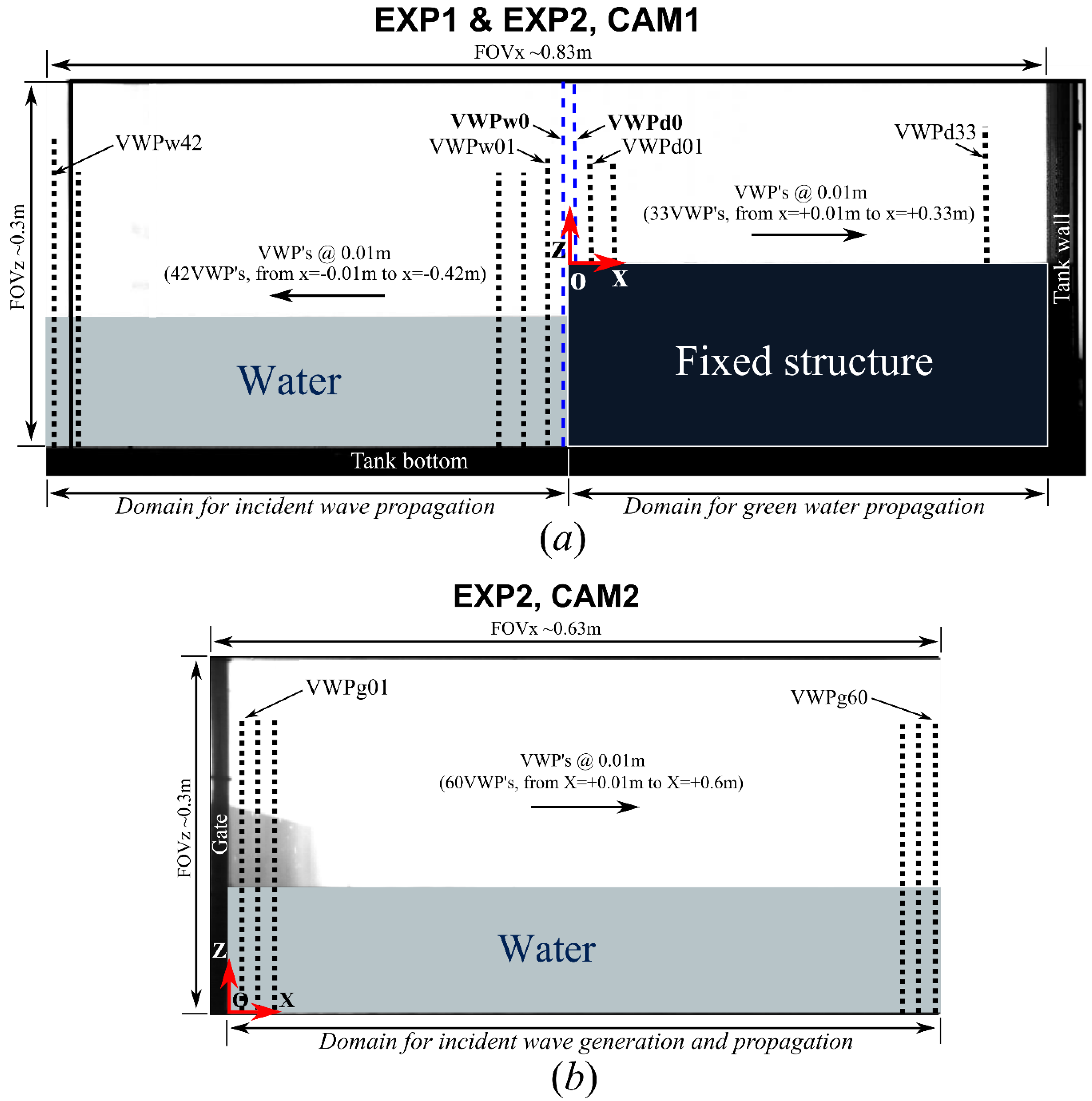
3.4. Image-Based Measurements

To capture the evolution of water in the stages of wave propagation downstream of the tank and green water on the structure, a high-speed digital camera (CAM1), model QUALISYS Oqus 310, was employed. This camera was used with an additional lens, AF DC-NIKKOR 105 mm f/2 D. The camera was set to 500 fps, with a resolution of 1284 × 1024 pixels. The camera was located to capture the side view of the tank, with the center view aligned to the bow edge of the structure, as shown in Figure 1b, for the experiment with the internal structure (EXP1). For the experiment without the structure (EXP2, Figure 1c), CAM1 was at the same place. A second camera (CAM2), model QUALISYS Oqus 110 was used in EXP1 and EXP2 to record the green water wavefront displacement and the wave generation stages during the gate aperture, respectively. For both cases, it was set at 200 fps, with a resolution of 640 × 480 pixels (Figure 1b,c). The software QUALISYS QTM was used to produce the videos.

3.4.1. Water Elevation Measurements

Measurements of water elevation were obtained from several virtual wave probes (VWPs), from the video made by the cameras that were parallel to the side view of the tank, that is, CAM1 for EXP1 and EXP2, and CAM2 for EXP2. To obtain the water elevation measurements, the open-source image-based methodology developed by [29] was employed. The methodology includes the three main stages of an artificial vision system: Image acquisition, processing, and analysis. These stages were implemented using open-source ImageJ software. Overall, gray-scale images were obtained from the video, then processed by intensity modulation and pseudo-color segmentation to obtain binarized images. Finally, through basic morphological operations, image analysis was carried out from the binary images to obtain water elevations at different regions of interest, which were recorded by the virtual wave probes (VWPs). See the work of [29] for more details regarding the procedures for image calibration, processing, and analysis to obtain the water elevation measurements.
For EXP1, virtual wave probes (VWPs) were located along the incident wave and green water propagation domains defined from CAM1, as shown in Figure 2a. This figure also defines the field of view (FOV) of the camera; ~0.83 and ~0.3 m in the x- and z-directions, respectively. A reference system of coordinates (xyz) was located at the beginning of the structure to locate the VWPs. Two VWPs were taken to measure the freeboard exceedance; VWPw0 and VWPd0, located at x = −0.005 m and x = 0.005 m from the origin. To monitor the water elevations on the deck, 33 VWPs, separated by a distance of 0.01 m, from x = 0.01 m (VWPd01) to x = 0.33 m (VWPd33), were used. To obtain the water elevations in the domain for the incident wave propagation, 42 VWPs, separated by a distance of 0.01 m were used, ennumerated as VWPw01 (x = −0.01 m) to VWPw42 (x = −0.42 m).
For EXP2, measurements were obtained for the same positions: VWPd01-VWPd33 and VWPw01-VWPw42, using CAM1. Furthermore, for CAM2 in this experiment, several VWPs were located along the domain for the wave generation and propagation defined in Figure 2b. In this case, the allowable FOV was ~0.63 m and ~0.3 m in the horizontal and vertical directions, respectively. A reference system of coordinates (XYZ), with origin at the gate, was considered to set 60 VWPs from X = 0.01 m (VWPg01) to X = 0.6 m (VWPg60), separated by 0.01 m.

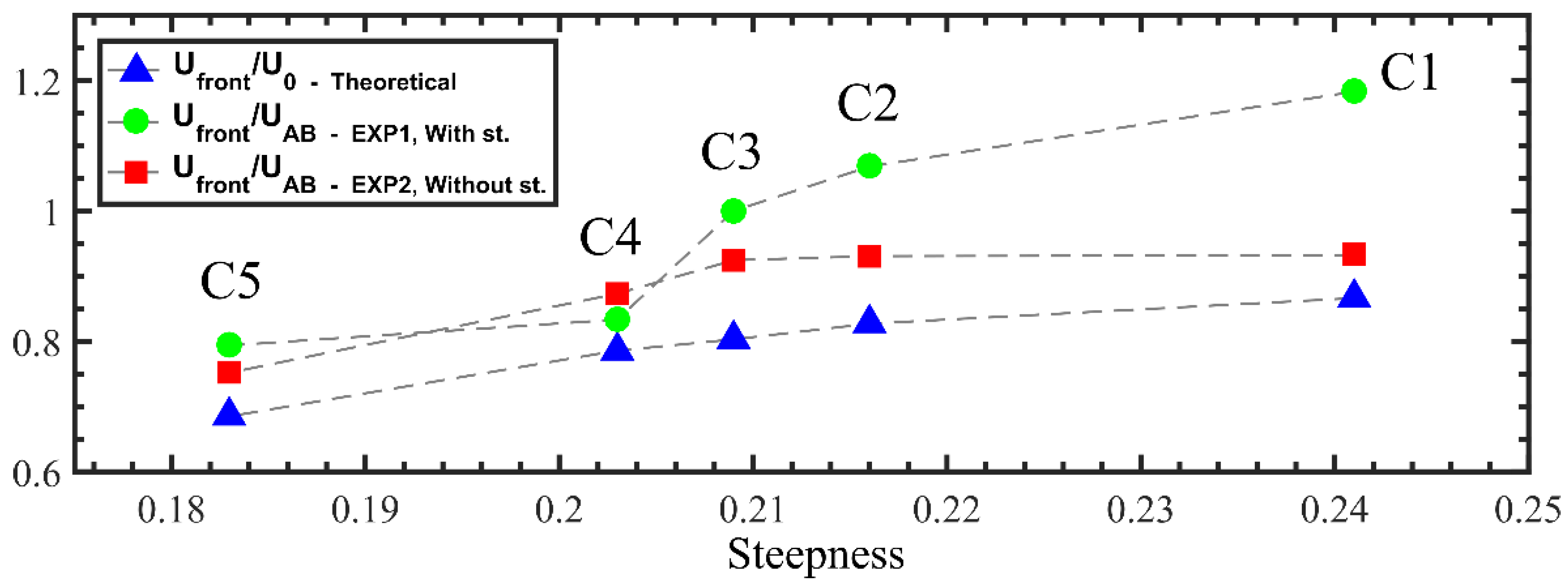
3.4.2. Wavefront Velocity

As stated before, CAM2 was installed parallel to the deck in EXP1 to capture the green water wavefront displacement (Figure 3). From the videos, the velocity of the wavefront (Ufront) was measured manually, using ImageJ visualization tools. The position of the wavefront edge was tracked every 0.01 s as water propagated over the deck. The movement of the green water wavefront may show cross-sectional variations along the width of the deck. Thus, for a practical measuring of its displacement, the spatial-average displacement over the cross-section line was monitored, starting from the instant at which the wavefront was first visible, close to the structure edge (Figure 3).

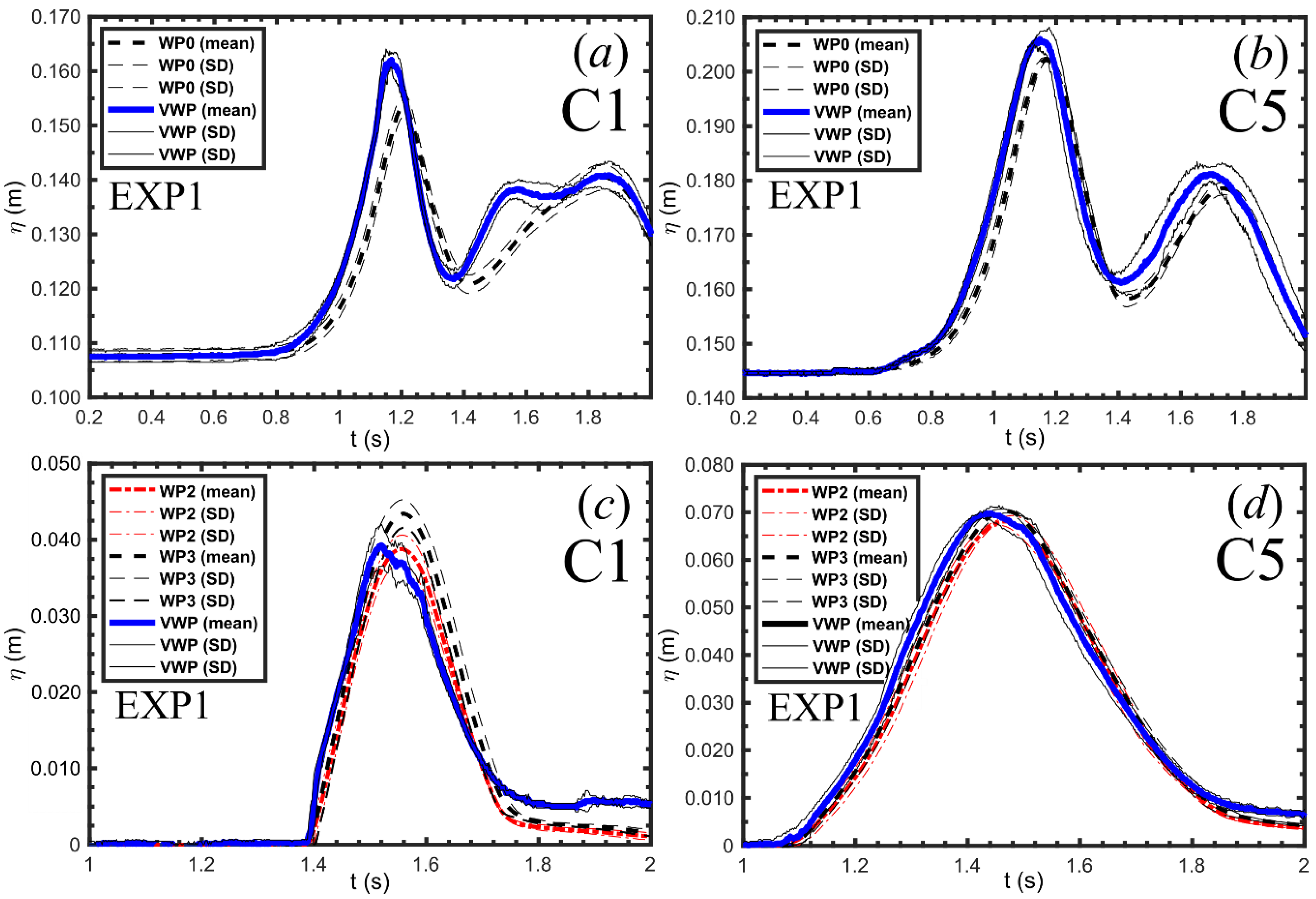
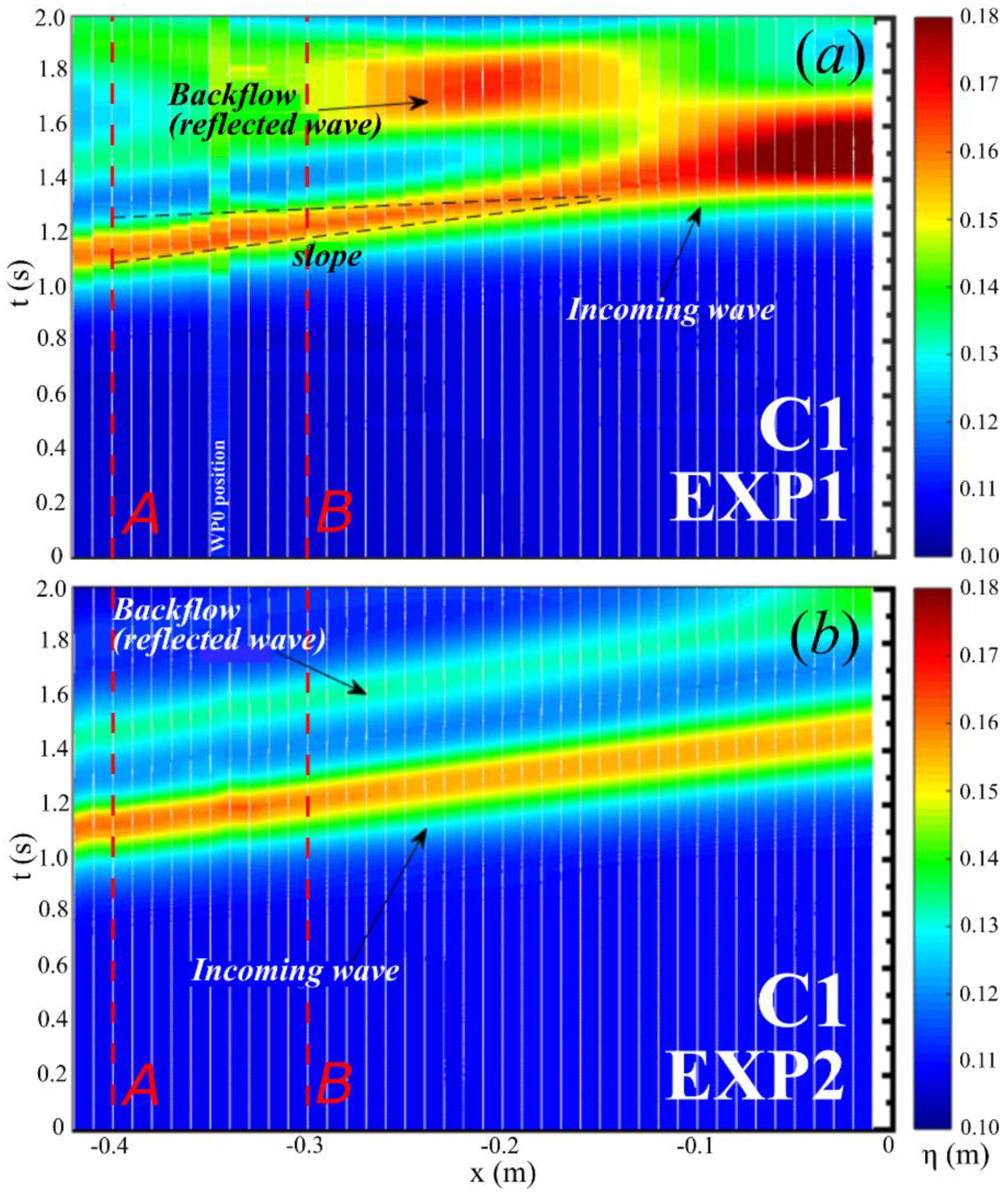
4. Comparison of Conventional and Virtual Wave Probes

The performance of the image-based approach to measure water elevations was verified by comparing the virtual results with the measurements given by conventional wave probes in the experiment with the internal structure (EXP1), considering C1 and C5 as representative of the other cases. Figure 4a,b show the comparison for the incident bore elevations between WP0 and a virtual wave probe, located at the same WP0 position, for C1 and C5, respectively. The signals shown in the figures are given in terms of mean and standard deviation values, obtained from the five repetitions. The VWP and WP0 signals have excellent agreement in measuring the static water level. A small shift in time is observed in the time series of the VWP with respect to WP0 for both cases, which can be partially related to the position of the camera, which was centered with respect to the bow edge of the structure. It is important to consider that WP0 measured the water elevations at the center of the tank, whereas the VWP monitored the elevations in the tank wall. Then, small 3D effects on flow observed in the wall might overestimate or underestimate the measurements at the center of the tank, which can explain the differences observed in Figure 4a,b. The agreement of the VWP with respect to WP0 is better for C5, which presented higher water elevations, following the trends of the incident and reflected waves.
On the other hand, Figure 4c,d show the comparison of the VWP measurements with those obtained with the conventional wave probes WP2 and WP3 installed above the deck, for C1 and C5, respectively. The VWPs were located about 1 mm upstream from the WP2 and WP3 position to allow image analysis, avoiding the obstruction of the sensors in the images. Note that the conventional wave probes indicate small 3D effects of the shipping flow, particularly for C1, as can be inferred from the differences in their maximum elevations (~0.004 m). These may be due mainly to installation issues of the conventional probes or a non uniform invasion of water over the deck. Overall, the VWP in C1 and C5 have reasonable agreement with water elevations over the deck measured by conventional wave probes.
Considering that the conventional wave probes can be subjected to different sources of error due to installation and performance (see, for instance, [1,29]), the applicability of the image-based approach was considered acceptable for the purposes of the present work.

5. Propagation and Characterization of the Bores

In this section, the results regarding the incoming bores are presented. These include the gate aperture, features presented during the generation and propagation of the bores, and a theoretical characterization of their steepness.

5.1. Gate Aperture

In the experimental dam-break approach, the gate aperture time (tr) should be as short as possible, to replicate a sudden gate release. To attain a suitable gate aperture time, the condition proposed by [30,31] for a dry dam-break experiment (i.e., h0 = 0, h1 > 0) was considered: t r < 2 / g / h 1 , where tr is the time for gate release, g is the acceleration due to gravity, and h1 is the initial water depth in the volume of water upstream of the gate.
From the video obtained with CAM2 in the experiment without structure (EXP2), the experimental gate release times, tr, were approximately 0.12, 0.13, 0.14, 0.15, and 0.16 s for cases C1, C2, C3, C4, and C5, respectively. These times were lower than the expected (i.e., design condition) tr values, indicating that the gate opening times for all the experiments were within the range defined above. It is important to mention that for the analyses described hereafter, the time t ≈ 0 s was considered as the time at which the trigger was activated. This was done to try to begin all sensor measurements almost at the same time. However, after triggering, the release of the gate took some milliseconds to occur, beginning its vertical displacement between 0.16 and 0.18 s in all the cases.

5.2. Bore Propagation
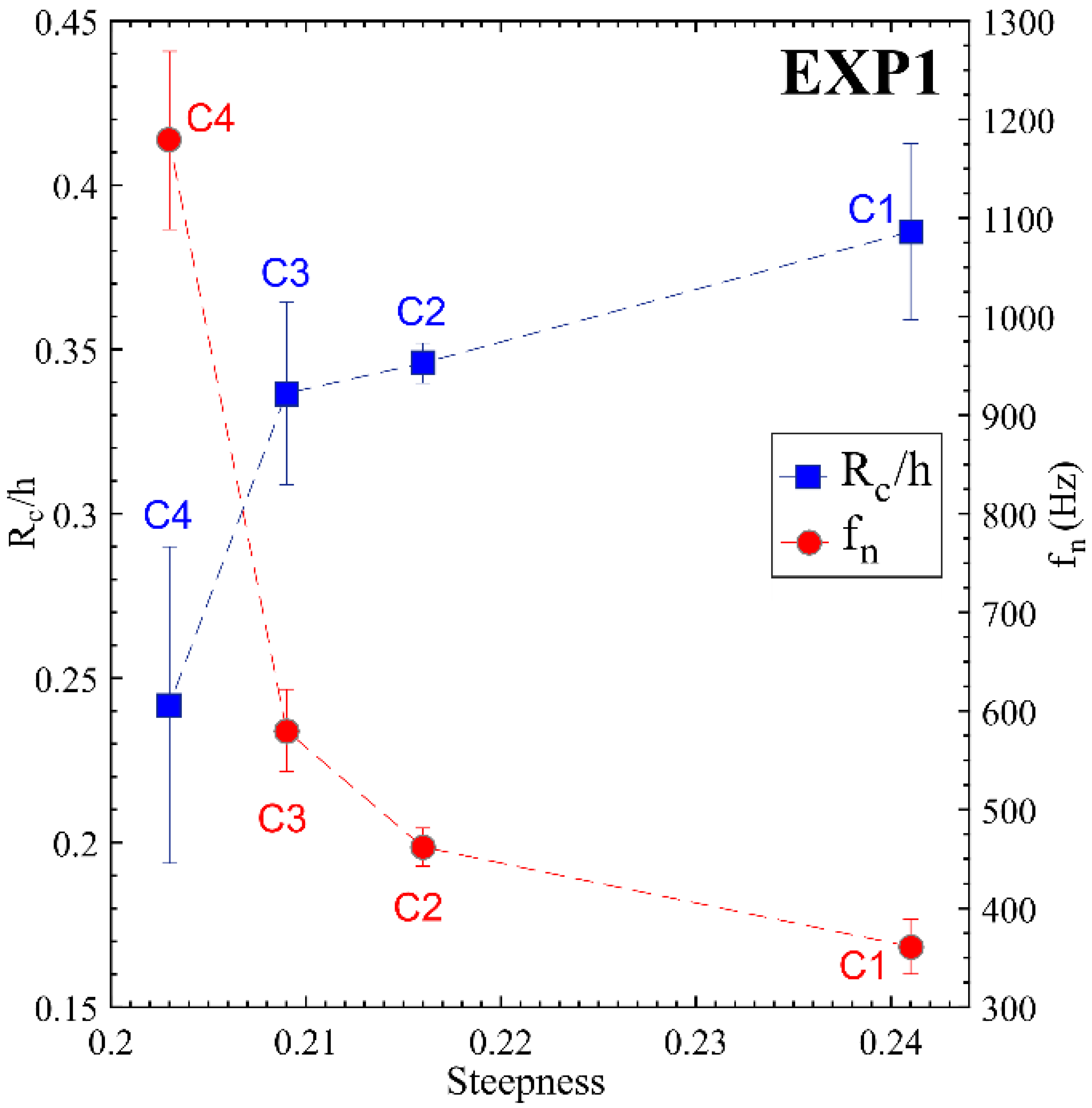
In the present methodology, when the gate opens, unbroken bores that propagate downstream are formed. For h0/h1 ratios lower than that of the present study (i.e., h0/h1 < 0.6), Stansby et al. [20] observed a mushroom-like jet after gate release. In the present case, some turbulence caused by the wave breaking over the downstream water volume and some drops of water falling from the gate were observed. Shigematsu et al. [32] suggest that the turbulence seen after gate release increases as the h0/h1 ratios drop. Furthermore, Liu and Liu [33] described that the resultant flow just after the gate release is commonly higher than the one observed when it developes farther from the gate, where water levels vary gradually.
To examine the transition of the bore development, from the gate area to some distance downstream, a spatial distribution of the water elevations was obtained from virtual wave probes from CAM2 (VWPg01-VWPg60, Figure 2b), as shown in Figure 5. This figure presents a comparison of bore profiles (i.e., water elevations, η, against the longitudinal positions from the gate, X) taken at various points in time (t1 = 0.35 s, t2 = 0.40 s and t3 = 0.75 s). The theoretical value, h2, estimated with the approach of Stoker (see Section 2) has also been included to make comparisons with the obtained results. The bore profile at t1 resembles a steep hydraulic jump, with amplitudes close to the theoretical ones of the Stoker model. Conversely, for later stages (t2), the shape of the profile changes their appearance to become an undular bore of greater amplitude. The crest of the bore was clearer as it propagated downstream. When its maximum elevation appeared, near X ≈ 0.42 m, the bore developed a trough and a second crest of smaller amplitude formed behind the first (t3 = 0.75 s). In this stage, the maximum elevation of the fully developed bore overestimated ~18% of the theoretical value, h2, obtained with the Stoker approach. These results showed that Stoker’s theory is more suitable for the hydraulic jump (shock wave) that appears after the gate release than for the fully-developed bore. This was also confirmed for the study cases C2–C5.
Considering C1, water elevation time series for the incoming bore were obtained from CAM1 at the positions defined in Figure 2a (VWPw01-VWPw42), allowing a two-dimensional flow visualization in time (t) and space (x), as shown in Figure 6. Figure 6a,b show the time–space distributions of water elevation at several positions (VWPw01-VWPw42) obtained from EXP1 (with structure) and EXP2 (without structure), respectively. For the case with structure, it can be noted that the bore propagated with an almost constant elevation (see the constant color region of the incoming bore until x ≈ −0.160 m), until the structure influenced it, increasing the elevations. These maximum elevations occurred just before the shipping of water onto the structure, in a stage known as bow run-up. Maximum values of ~0.196 m are seen close to the structure (x ≈ −0.01 m), defining the maximum freeboard exceedance of the event, which is one of the main parameters in green water analyses (see Section 6.2). Next, a reflected wave is seen to be generated by the structure just after the incoming bore reached its maximum value, during the bow run-up stage (for t > 1.6 s at x ≈ −0.2 m). The reflected wave has a maximum elevation of ~0.167 m, which is ~15% lower than that of the incident wave. In contrast, for the case without a structure (Figure 6b), specific regions of maximum elevations due to bow run-up and backflow are not seen. Instead, continuous color regions for the incident bore and a wave reflected by the tank wall are observed, suggesting that they propagate with almost constant elevation and velocity (see the slope of the colored regions). It is important to comment that in studies perfomed with wave trains, the backflow generated after bow run-up may significantly affect the features of after-coming waves. In these cases, the resultant green water events may be dependent on the backflow generated from previous wave interactions with the structure [7].
Results indicate that the structure presence has an influence on the features of the incoming bore, which is more noticeable close to the structure. Similar features were observed for C2–C5, differing mainly in the magnitudes of the incoming and reflected waves. Relationships between these waves and the resultant water on deck are further described in Section 6.

5.3. Bore Steepness

In order to characterize the incoming bores, their steepness has been estimated theoretically. To do this, they were assumed as solitary waves, which can be described by two parameters: Wave height and water depth [34]. For all the study cases, these parameters were considered from the mean values obtained in the time series of water elevations measured at point A for EXP1 (VWPw40, Figure 6a), considering the five repetitions. From these time series, the water depth parameter was considered as the mean value of the measured h0 values (i.e., h ¯ o ), whereas the wave height parameter was considered as the difference between the mean maximum amplitude in the VWPw40 time series and h ¯ o (i.e., H ¯ ). The steepness of each bore was calculated as ϵ = H ¯ / L T , where LT is the theoretical length of the solitary wave, which was estimated as [35,36]: L T = 1.5 h ¯ 0 ( H ¯ / h ¯ 0 ) 0.5 . The H ¯ values measured for C1, C2, C3, C4, and C5 were ~0.055, ~0.056, ~0.058, ~0.059, and ~0.060 m, respectively, whereas the corresponding steepnesses were ~0.241, ~0.216, ~0.209, ~0.203, and ~0.183. These values suggest that the bores have almost the same height, H ¯ (varying ~5 mm from C1 to C5), differing in length, which increases from C1 to C5. The incoming bore in C1 is the steepest of all cases; however, it has to be noted that all the bores used in this work present a close variation in steepness ( 0.183 < ϵ < 0.241 ), that is, the interaction of very steep waves with the structure was not considered.

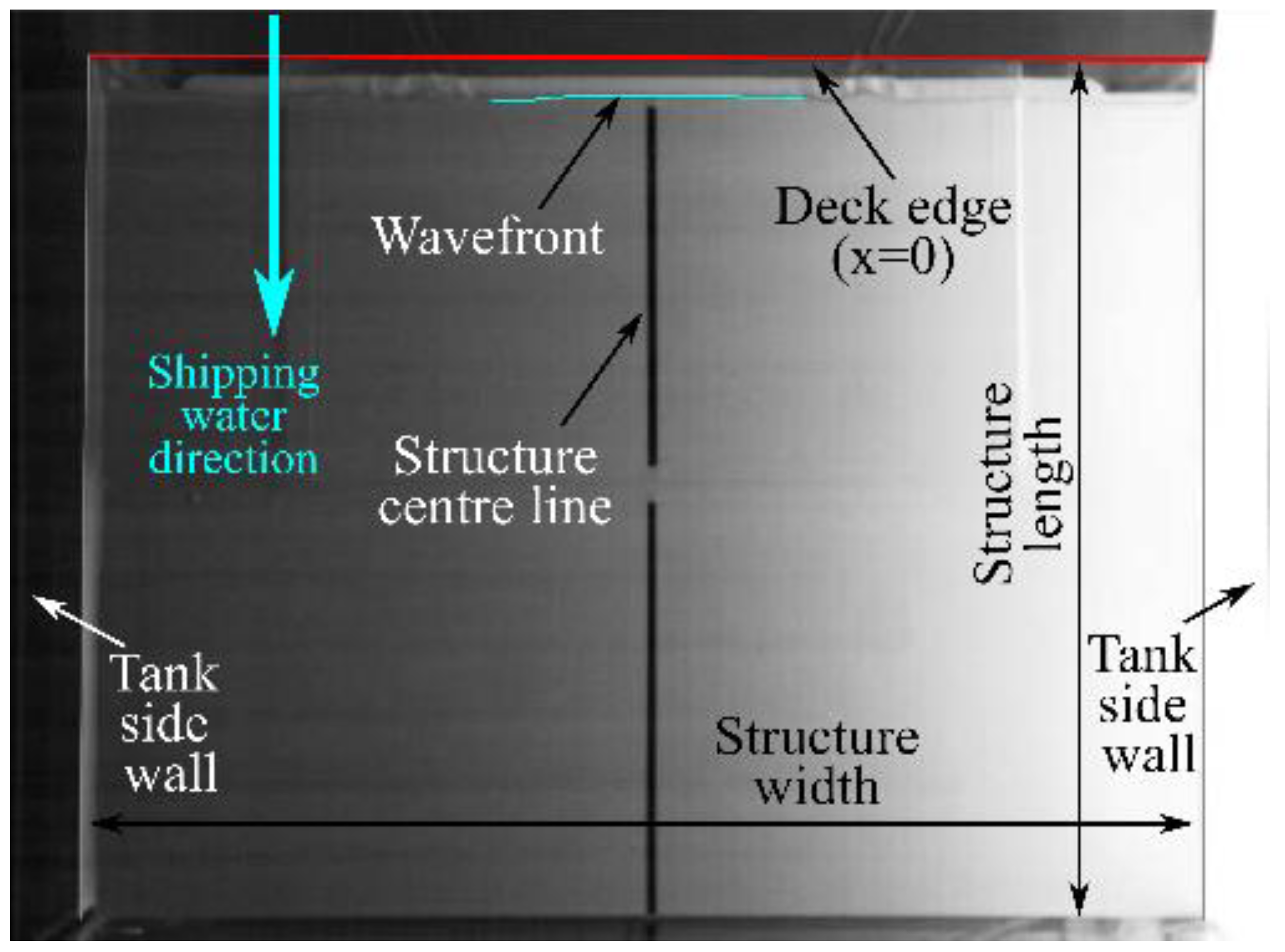
6. Interaction of Bores with the Structure: Green Water

This section presents the experimental results of the green water events originated from the interaction of the incident bores with the structure. First, main stages of green water for the representative case C1 are illustrated, emphasizing details of an air cavity occurring in the early stage of the event. Then, the evolution of green water elevations is treated similarly to that in Section 5, where temporal and spatial distributions were given for the incoming bore. Finally, some relevant parameters in green water research, such as freeboard exceedance and wavefront velocity over the deck, including their relationship with the incident bores, were analysed.

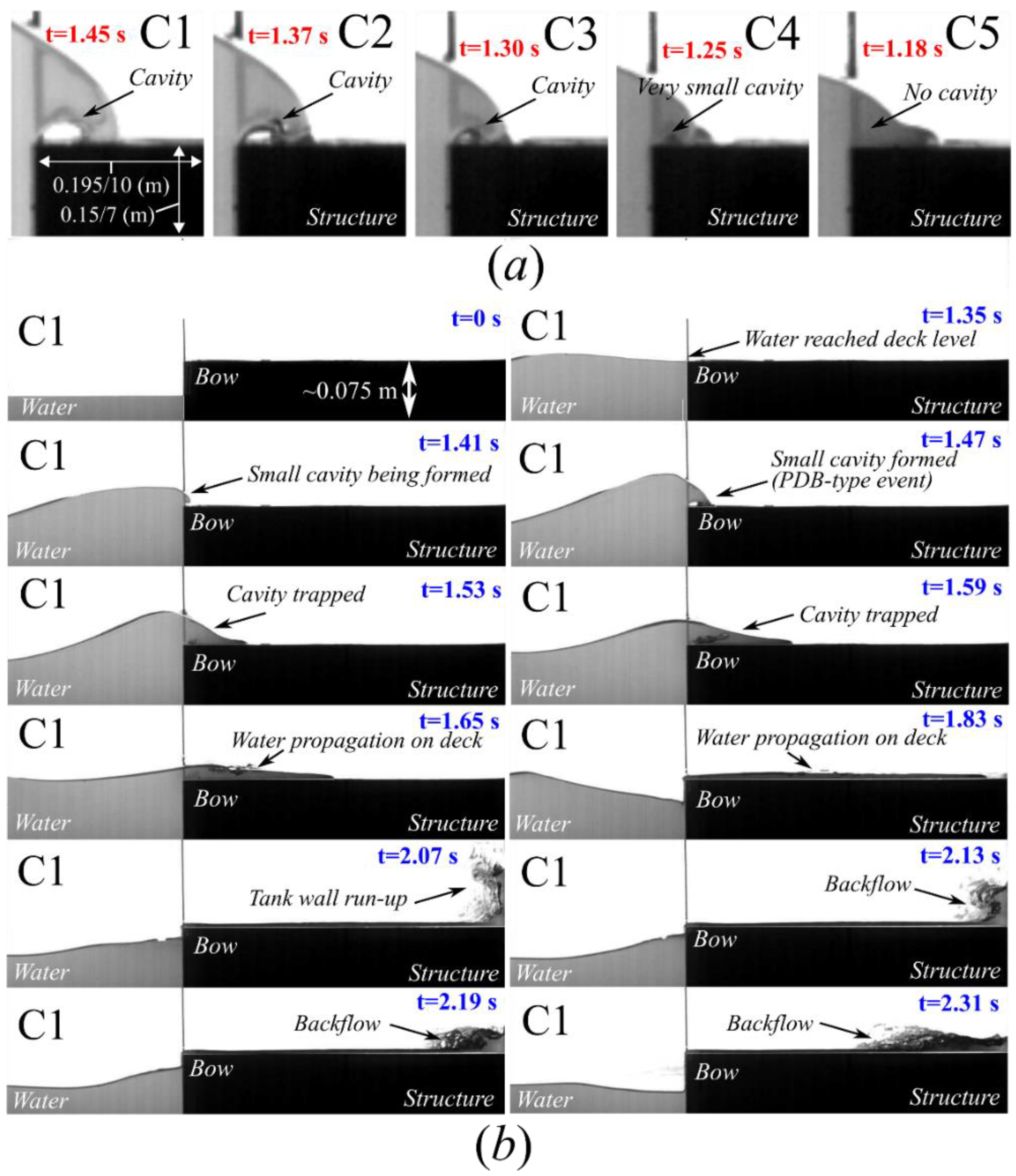
6.1. The Green Water Events
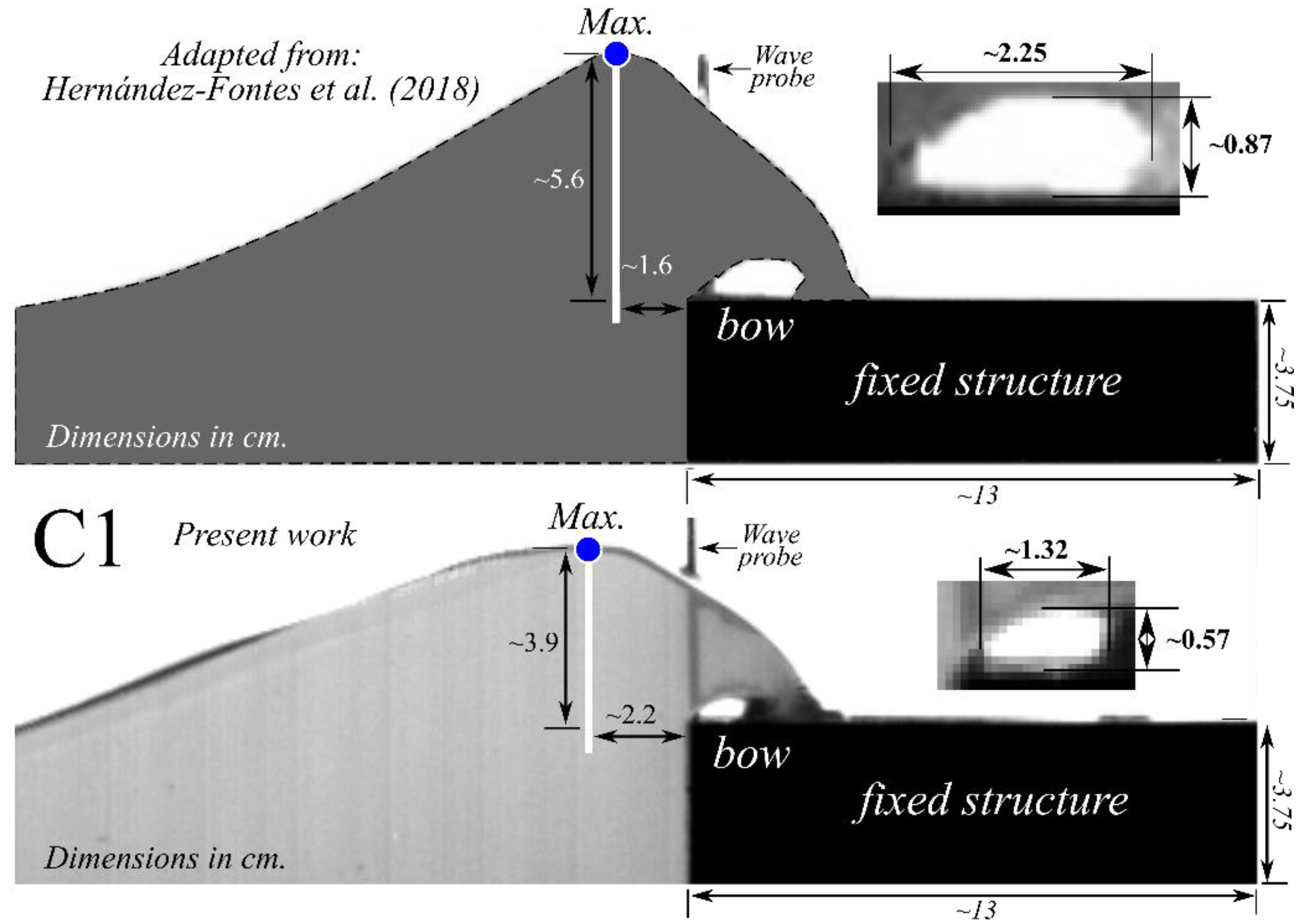
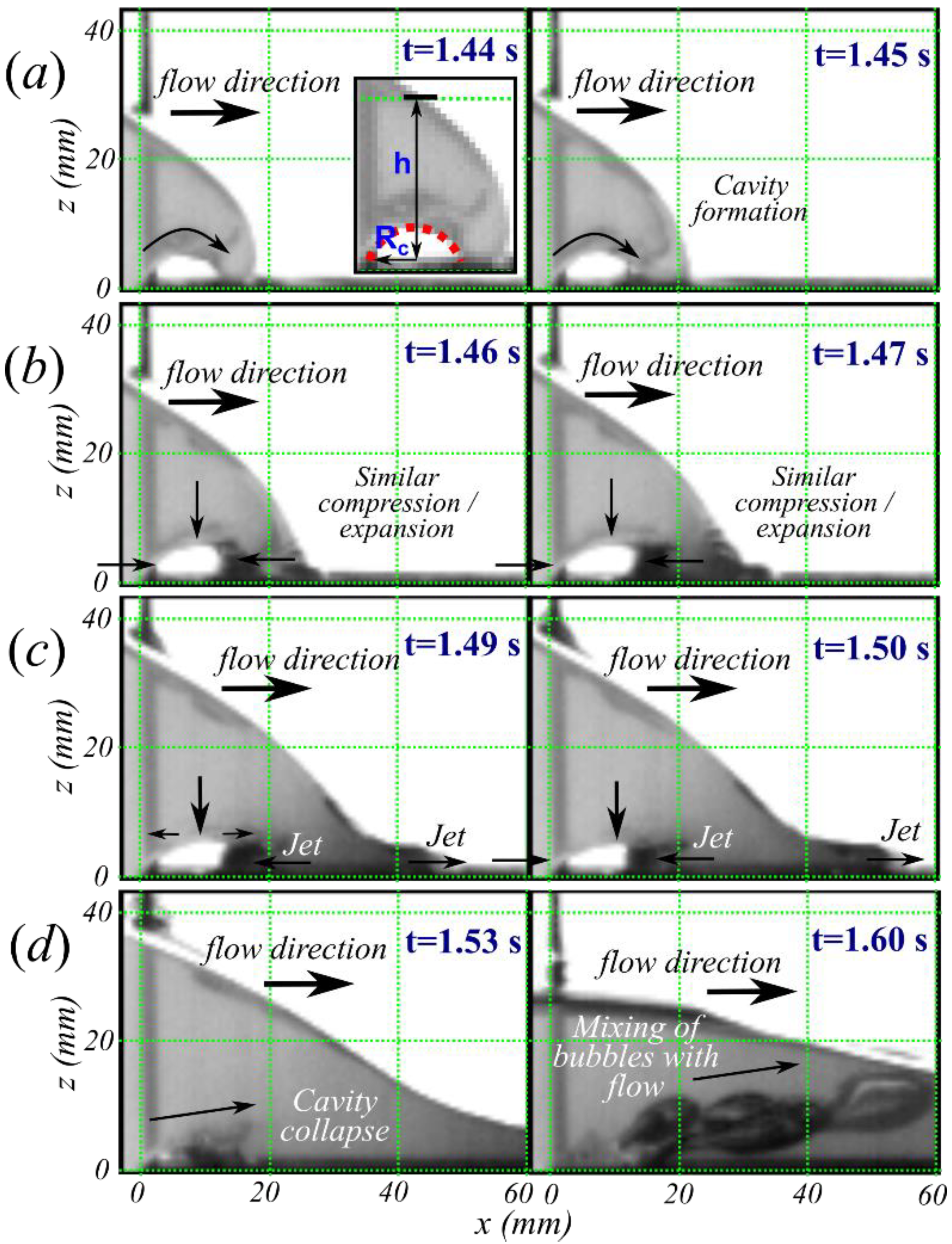
The green water events obtained for C1, C2, C3, and C4 presented the formation of a small air cavity at the beginning of the deck, whereas C5 did not presented such a cavity (see the initial stages shown in Figure 7a). The cavity size reduced from C1 to C4. From a qualitative point of view, the events obtained in C5 and C1–C4 can be classified as dam-break (DB) and plunging-dam-break (PDB) types of green water, resembling the ones obtained with regular waves on a fixed structure, as reported by [7]. In this section, the event of C1 presented the largest air cavity of all the PDB events found, then it was considered for reference to describe some details of water behaviour on deck. Figure 7b shows some stages of the green water event found in C1. Snapshots capture the flow at different points in time, including the initial (bow run-up) and final (backflow) stages of green water.
The features observed in the event found for C1 (Figure 7b) were also found by [15], using the same initial conditions for green water generation (h0/h1 = 0.6, FB = 0.042 m), in a smaller experimental installation (~1 m long, ~0.335 m wide). The installation of [15] had the same upstream reservoir length, and the same height for the fixed structure. The main differences are related to the distance available for the bore development and the tank width (~2.49 and ~1.49 times greater in the present work, respectively). Figure 8 presents the comparison between the green water patterns obtained in these two works. The patterns were captured 0.12 s after the water level reached the height of the deck. Note that both cases resemble the PBD-type of green water described by [1,7]; where an air cavity is produced while two small jets are formed as the wave front touches the deck. However, in [15], the cavity was larger (~1.7 and ~1.5 times in the horizontal and vertical directions, respectively) and the maximum elevation of the wave was higher (~30%) and occurred closer to the bow (~38% closer) than in the present work. Reduction in the cavity sizes with respect to the cases presented in [15] were also verified for cases C2, C3, and C4. The shorter distances for bore development due to the smaller tank used in that work may have influenced the increase in wave amplitudes because of the reflection effects, and in turn, the generation of larger cavities.

Air Cavity Analysis

The study of the evolution of air cavities formed during wave interactions with marine structures is important since it may yield information about the induced loading on the structure. Some authors have stated that the presence of trapped air increases the loading on the structure, whereas others claim that the trapped air delays the impact [37]. For the case of cavities formed during green water events, Colicchio et al. [38] performed a detailed analytical and numerical investigation, evaluating scale effects in the cavity formed during PDB events obtained with regular waves. Alternatively, in this work the air cavities formed during the present PDB-type green water events (C1–C4) are analysed in a simplified way through analogies made with the air cavity formed in a vertical wall during some types of flip-through events (i.e., flip-through “Mode B”, [37,39,40]). In these events, there is the formation of an air cavity due to the overturning of a wave crest approaching the vertical wall (the focusing stage). The cavity is subsequently closed, due to the generation of an upward jet, which meets the wave crest. Then, the cavity collapses and the jet rises above the wave crest [37]. Despite the kinematics of the entrainment mechanism of both the flip-through and green water problems is quite different, it is possible to relate some concepts from that phenomenon [39] to partially describe the evolution of the cavities formed in the present green water events as follows:
(1)
The air cavity is entrapped against a horizontal surface rather than a vertical wall (Figure 9a).
(2)
The deformation of the air cavity (i.e., compression and expansion) is very similar in the horizontal and vertical direction, that is, it suffers an isotropic compression and expansion (Figure 9b).
(3)
The air-cavity deformation occurs mainly in the horizontal direction, that is, it presents an anisotropic compression/expansion due to the increase in the water column above it. However, in the present case, the cavity is also reduced by the effect of the backward jet that is formed as water propagates down the deck (Figure 9c).
(4)
The air cavity collapses and fragments in small bubbles that mix downstream with the advancing flow (Figure 9d).
Lugni et al. [37] suggest the importance to evaluate the dynamic behavior of the air cavity, which shows high frequency oscillations before it collapses. This may be relevant to study structural loading effects, since structural vibrations, ventilation, and cavitation may be induced [39]. Thus, it is important to estimate its resonance frequency. The effect of this frequency in loading is out of the scope of this work. However, we practically evaluated it for each study case from an analogy made from the flip-though events. This can be done approximately by considering the air cavity as a two-dimensional bubble of semicircular cross section with a radius, Rc, during the initial stage of its formation, as soon as the tip of the plunging wave reaches the deck, as illustrated in Figure 9a. It is assumed that this cavity behaves like a harmonic oscillator that vibrates at a resonance frequency, fr, when it is subjected to an impulsive force. Moreover, effects due to surface tension, dissipation, and damping must be ignored [37]. With these assumptions, fr can be estimated as [37,41]: f n 2 = γ p / 2 π 2 ρ R c 2   l o g ( R c / 2 h ) , where p is the atmospheric pressure (~101.3 kPa), ρ is the water density (1000 kg/m3), γ ≈ 1.4 is the specific heat ratio (disregarding the effect of heat conduction from the bubble), and h is the distance from the center of the cavity at the vertical wall to the free surface (in the flip-through problem). For the present application to green water, h is assumed as the distance from the center of the cavity at the deck to the free surface (h ≈ 0.02 m, Figure 9a).
Figure 10 presents the ratios, Rc/h, and the theoretical fr values obtained for different steepnesses (C1–C4). The results are shown in terms of mean and standard deviation values. Note that for lower steepnesses, the cavity radius, Rc, is smaller in relation to the height, h. Conversely, for these steepnesses (cases with smaller cavities), the theoretical resonance frequency, fn, is larger than those obtained for the cases with larger cavities, which were generated with steeper bores and higher freeboards (e.g., C1 and C2).
Although the physics of the cavity formed during a green water event is different from that of a flip-through phenomenon in a vertical wall, the present analysis could be considered as a practical alternative to analyse the dynamic behavior of the air cavity formed in green water events of the PDB-type.

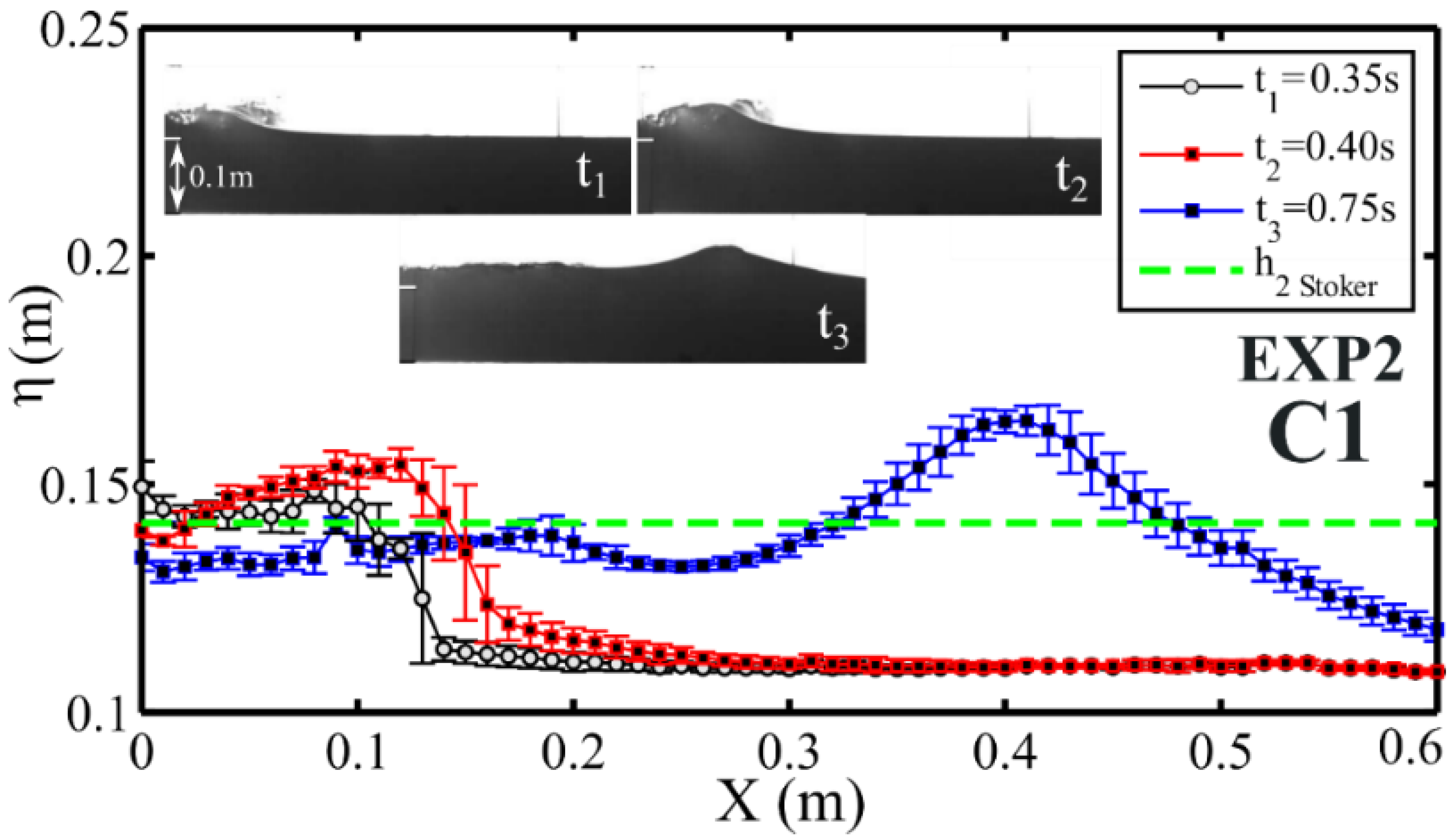
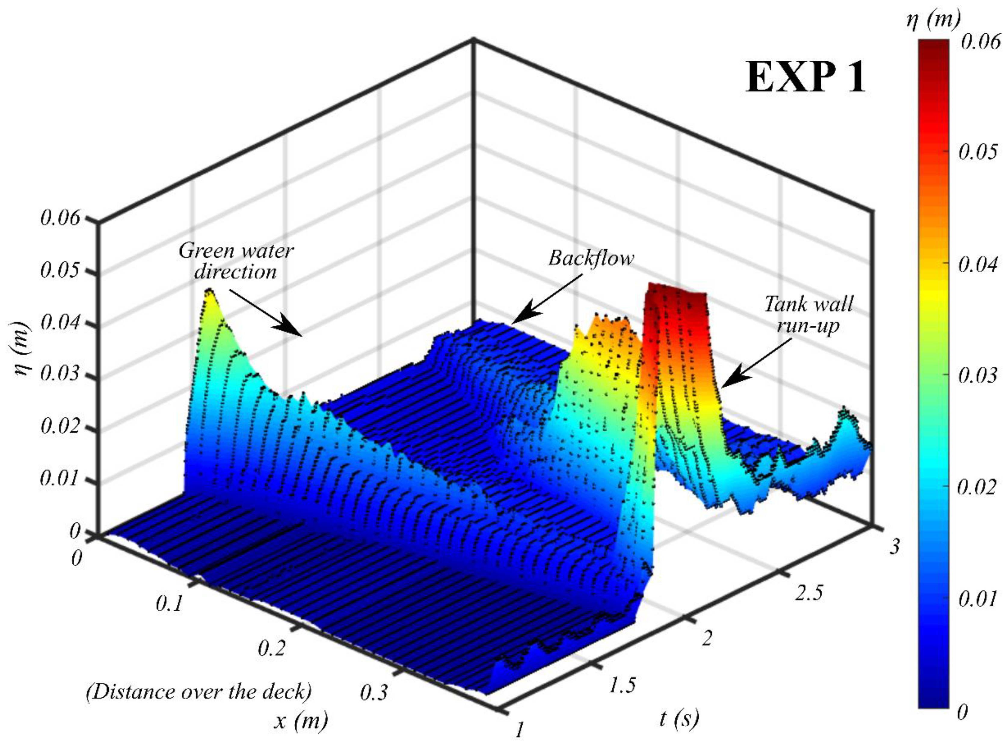
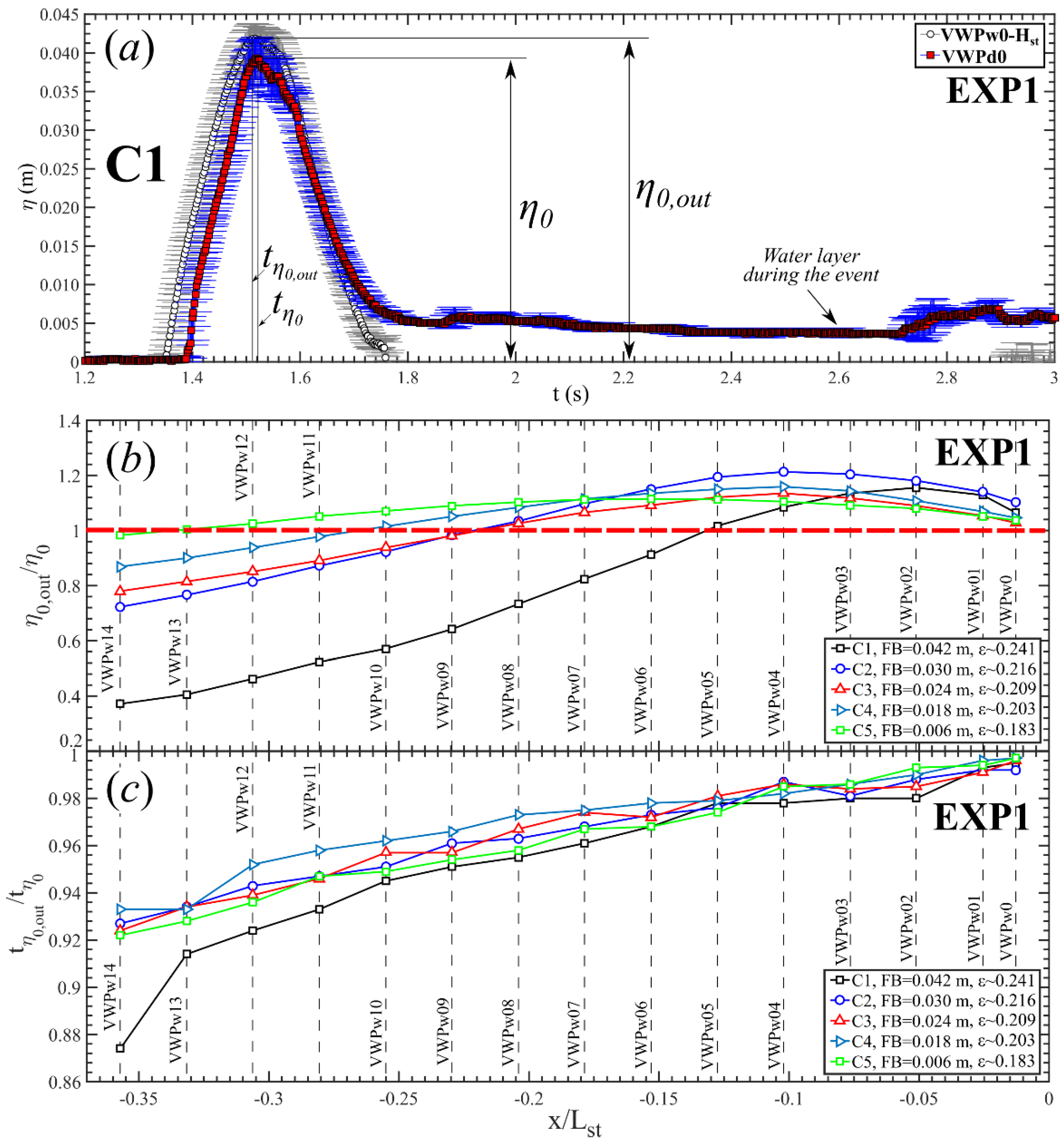
6.2. Green Water Elevations

There are few experimental measurements available in the literature of the time series of green water elevations on the deck of a structure, considering several positions. To obtain these measurements it is common practice to use some conventional wave probe arrangements to extract water elevation data. Even in a two-dimensional setup, green water elevations have been measured by obstructive wave probes (e.g., [1,7]). Besides interfering with the flow propagation, these sensors yield information for very few positions on the deck, limiting the understanding of the water´s spatial evolution. This is valuable information for comparison or validation of analytical and numerical models.
The time series of green water elevations on the deck for C1 are shown in Figure 11. These were obtained for one of the five repetitions from virtual wave probes located along the deck (VWPd01-VWPd33, Figure 2a). Water evolution is shown for the complete duration of the experiment (3 s). However, it is important to consider that the range of applicability of the 2D image-based procedure is until ~2 s, before the tank wall run-up, where 3D effects are presented. Data processed for t > 2 s are shown for illustrative purposes to have an idea of flow behaviour during tank wall run-up and backflow. The evolution of the cavity that is formed in the present green water event was disregarded in the analyses.
Three main stages can be identified in Figure 11: First, the deck was completely dry (x = 0, 0 < t < 1.2 s), until a finite amount of water was shipped onto it and propagated to its end (x = 0.392 m, t ≈ 1.8 s). The water then interacted with the tank wall, causing run-up (t > 1.8 s). Finally, the run-up water fell down due to gravity and backflow occurred on the deck (see the stages shown in Figure 7b). The stages observed in this case were also identified for the other cases, which presented larger amounts of water over the deck.
As an alternative to previous two-dimensional techniques to study water evolution on deck (e.g., [1]), the present approach can be extended to to acquire time series of green water elevations at several positions over the deck for different setups.

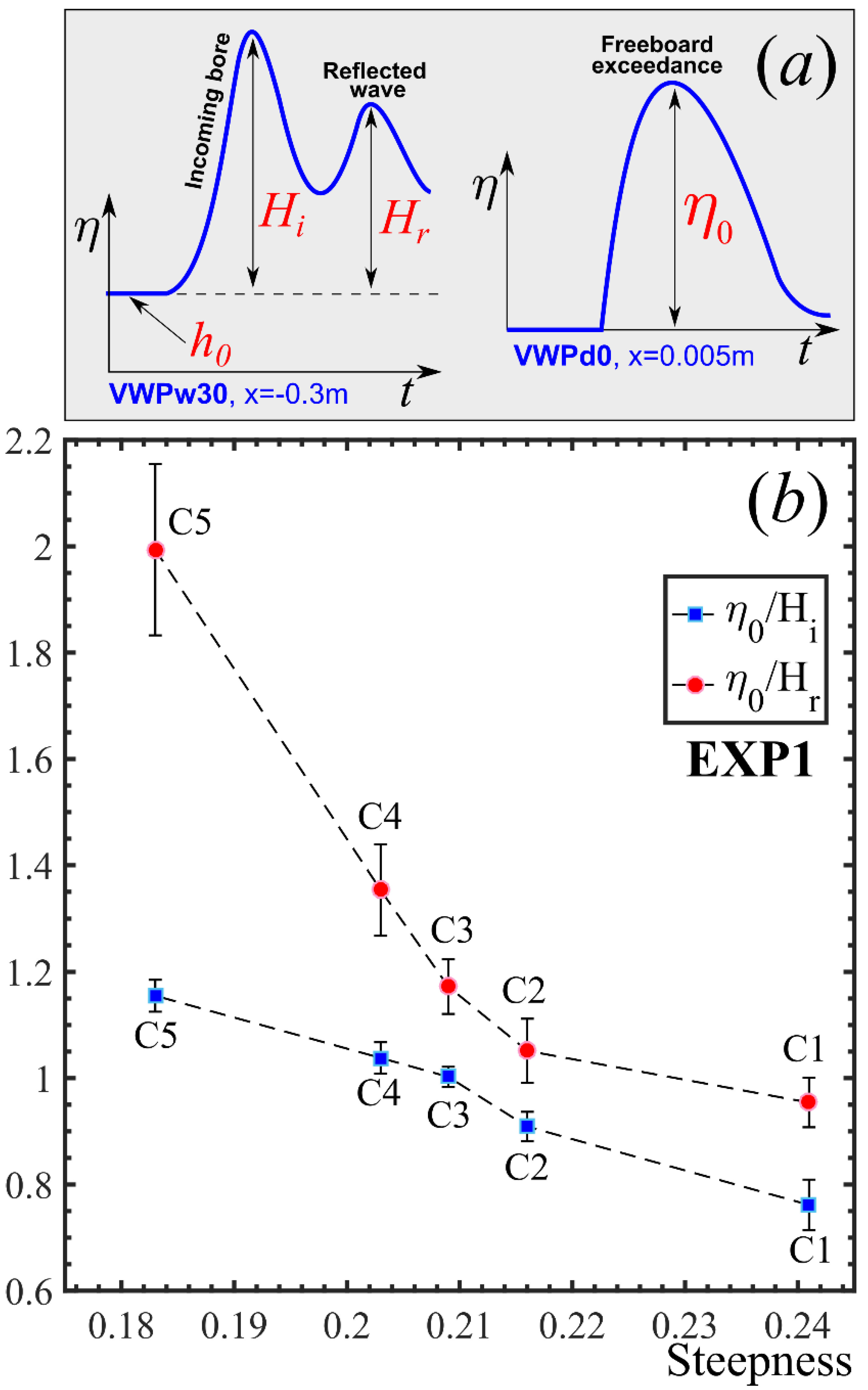
Freeboard Exceedance

One of the most important parameters in the study of green water events is the freeboard exceedance time series, or the effective water elevations from the incident wave that represent the volume of water that ships onto the deck. The maximum value of these series is known as the maximum freeboard exceedance (η0, Figure 12a), and it is commonly considered as input of analytical (e.g., [24,42]) or numerical (e.g., [43]) models to study green water propagation over the deck. However, not every freeboard exceedance produces the same water elevation over the deck [44]. The water elevations measured outside the deck may be higher than those measured on it [45].
Experimentally, the freeboard exceedance has been measured over the deck of simplified structures at positions very close to the deck edge (e.g., [1]). However, in more complex arrangements, such as ship-type structures, it has been necessary to install the wave probes outside the hull to monitor the relative deck-wave motions (e.g., [42,45,46,47,48]). Details of the exact location of the wave probes with respect to the edge of the deck are scarce in most works. However, a typical distance can be inferred from the studies of [49,50], who used wave probes ~1 cm off the bow to measure relative ship-wave motions.
Figure 12 shows the relationship of the maximum freeboard exceedance (η0) with the maximum elevations of the incoming bore (Hi) and of the wave reflected by the structure (Hr), considering EXP1. Hi and Hr were measured at the position of point B defined in Figure 6 (VWPw30, x = −0.3 m), whereas η0 was measured at 5 mm from the bow edge (VWPd0), as illustrated in Figure 12a. Figure 12b shows the ratios, η0/Hi and η0/Hr, for different bore steepnesses. First of all, note that from C1 (higher freeboard, steeper bore) to C5 (lower freeboard, longer bore), the values of η0 range from ~80% to ~120% of the values of Hi. For C3, η0 is almost the same as Hi. Rearding the reflected wave, η0 is very close to Hr for C1 and C2; however, for longer bores and shorter freeboards (from C3 to C5), η0 overestimated Hr, reaching values of ~200% the values of Hr for C5.
In this study, we evaluated the differences obtained when selecting freeboard exceedance at the beginning of the deck and at some distances upstream (Figure 13). Although the present work does not apply to all green water problems found in real cases, this type of analysis may be extended to estimate correction factors in cases where green water studies were performed with freeboard exceedance data obtained outside the deck. Regarding the present application, we made a comparison between the resultant VWP time series obtained from VWPw0 (x = −0.005 m) subtracting the structure height (i.e., VWPw0-Hst, with Hst as structure height) and the time series measured on the deck (VWPd0), as shown in Figure 13a. The time series include the mean and standard deviation values estimated from all the repetitions. It is observed that the trend of both series is very similar, despite very small shifts in time between them and some differences in water elevations, mainly at the tail of the curves for t > 1.7 s, where the VWPd0 presents almost constant elevations. These elevations are due to a layer of water remaining at the edge of the deck during the event (see snapshots in Figure 7b). Considering the time at which the water elevations started rising, the time difference was about 0.03 s between both series.
In Figure 13a, the maximum freeboard exceedance of the time series taken upstream the deck edge (i.e., η0,out) overestimated that of VWPd0 (η0) by approximately 7%. These maximum values occurred at the time t η 0 , o u t and t η 0 , respectively, which presented a very small time difference of about ~0.002 s.
Figure 13b,c show, respectively, the variation of the ratios η0,out0 and t η 0 , o u t / t η 0 at several positions (x/Lst, where Lst is the structure length) upstream the bow edge for all the study cases. The parameter, η0,out, was obtained from the mean values of time series provided by VWPs at these positions, substracting the structure height. In Figure 13b, it can be noted that for each case, there is a region from the structure at which η0,out overestimated between 10% and 25% of the freeboard exceedance over the deck (η0), which avoids underestimation of values measured over the deck. However, there is a region in which η0,out starts underestimating η0 (see [η0,out/η0] < 1 in the figure). The condition η0,out < η0 is accomplished at shorter distances from the structure for the cases with higher freeboards (steeper bores) and at longer distances for the lowest freeboards (longer bores).
It is also important to analyse the difference in time at which η0,out and η0 occurred, as shown in Figure 13c. This difference will increase as the freeboard exceedance is considered farther from the structure. All cases presented this behaviour, showing differences between t η 0 , o u t and t η 0 of ~3% tto 7% for a distance about 25% of the length of the structure.
Disregarding the differences observed in the time series of freeboard exceedance measured outside and over the deck, the former could be considered for practical applications if a suitable range is considered to avoid underestimation of η0. For other applications, including oscillatory motions of the incident flow or motions of the structure, it may be relevant to verify suitable regions to estimate η0,out in order to avoid underestimation of the resultant water on deck and to reduce the shifts in time in simulations. Perhaps, it should be necessary to consider a correction factor in the estimation of the η0 parameter.

6.3. Green Water Kinematics

The present methodology also includes the measurement of the wavefront velocity, Ufront, which is another important parameter in green water research. It is used mainly to estimate the horizontal loading in structures located over the deck [2]. Information about this parameter has been extracted from visual inspection of the wavefront edge displacement onto the deck, as described in Section 3.4.2.
Mean Ufront values for the five study cases were calculated considering different domains over the deck. These values were obtained by applying linear regression analyses to the wavefront velocity data for different domains in x, considering x = 0 at the bow edge. At the early stages of green water occurring at the beginning of the deck, Ufront was between 0.29 and 0.31 m/s and 0.38 and 0.44 m/s for the domains 0 < x < 0.02 m and 0 < x < 0.05 m, respectively, for all cases. Next, when the wavefront developed further over the deck, all cases reached Ufront values between 1 and 1.1 m/s (0.1 < x < 0.35 m). It was verified that the wavefront presented acceleration over the deck, from Ufront ≈ 0.2–0.3 m/s to Ufront ≈ 1.1 m/s for all cases. The velocities found for the well-developed wavefront are of similar orders of magnitude to those reported globally by [1], for green water experiments with regular waves in a wave flume.
Figure 14 presents the relationship between mean values of the well-developed Ufront (measured between 0.1 < x < 0.35 m) and kinematics of the incoming bores. To do this, ratios of Ufront with the bore front velocity estimated teoretically (U0, Stoker) and with the bore front velocity calculated experimentally (UAB) for the cases with (EXP1) and without the structure (EXP2) are presented. UAB was calculated from EXP1 and EXP2, considering the domain defined by x = −0.4 m (point A) and x = −0.3 m (point B) (Figure 6) as UAB = (xBxA)/(tBtA), where xBxA is the distance between points A and B, and tA and tB are the points in time at which the mean maximum elevation occurred in A and B, respectively.
For the velocities obtained with the experiments without a structure and calculated theoretically, Ufront was always lower than the bore front velocity. However, for the case with the structure, Ufront was closer to UAB, particularly for C2 and C3. For C1 (steeper bore), Ufront was ~20% higher than UAB, whereas for C4 and C5, it was ~20% lower.
On the other hand, it can be noted that the theoretical values for the bore velocity (U0) overestimate the experimental ones (UAB, EXP1, and EXP2) for all cases, being closer to the ones obtained for EXP2 (case without the structure). Thus, it can be inferred that the presence of the structure reduced the velocity of the incoming bores. This suggests that it might be wise to consider a correction factor in green water analyses that employ kinematic information from the undisturbed incident wave.

7. Conclusions

The study of green water on structures requires detailed systematic experimental analyses that allow green water patterns to be identified and analytical or numerical models to be validated.
Considering the interaction of wet dam-break bores with a fixed structure, this paper presented an alternative image-based experimental study of green water. The experiments had a duration of ~3 s, which allowed the use of high sampling rates in cameras to capture details of wave propagation and green water flow, using two-dimensional open-source image-based methods.
The main conclusions of this work are summarized as follows:
-
Five different study cases were performed, considering the same wet dam-break ratio h0/h1 = 0.6 and five different freeboards (0.006 ≤ FB ≤ 0.042). These conditions generated undular bores with similar heights (0.055–0.060 m for all cases) and theoretical steepnesses in the range 0.183–0.241. These bores generated four green water events with small cavities formed at the beginning of the deck (PDB-types of green water) for the steeper bores and a case where no cavity was observed (DB-type of green water) for the longest bore. Some concepts used to analyse the cavities formed in flip-through events in vertical walls were introduced in the present work to practically describe the evolution of the PDB cavity in a practical way.
-
The consideration of the maximum freeboard exceedance (η0) is important in the implementation of analytical and numerical models. In this study, it was verified that selecting η0 at some distances outside the deck may yield differences with respect to the one measured at the bow. It is suggested that for applications in which the relative wave-deck motions were considered outside the deck, a correction factor should be estimated and included to approximate the real freeboard exceedance that occurs at the edge of the deck, considering also its time of occurrence, which is relevant to green water simulations.
-
The proposed experimental setup allowed the use of image-based methods available in the literature to analyse the temporal and spatial evolution of the incident wave and green water on deck in a two-dimensional framework. This is an advantage over traditional techniques that employ obstructive wave probes over the deck to monitor green water elevations at a few positions. Regarding these results, a database of water elevations has been made available to allow model validations by other authors. These include time series of water elevations for the five repetitions of the five study cases, considering the experiments with and without the fixed structure. The database was made available in a Mendeley data repository: http://dx.doi.org/10.17632/zjrsmffh4d.1 as Supplementary Materials.
The physics of the wet dam-break bore used in the present method is different from that of regular waves, which are commonly used in green water analyses. However, it may be an alternative to acquire systematic and high-resolution local details of water propagating over the deck due to the small duration of the experiments. With tests of small duration, the sampling frequency of cameras could be significantly increased, and the high-speed visualization could be performed in a repeatable and reproducible way. The method can be extended to analyse more types of green water events, including the systematic analysis of other magnitudes, considering different types of wet dam-break waves (e.g., broken, unbroken) by changing the h0/h1 wet dam-break ratios. Moreover, different structure configurations can be tested, such as rounded or sloped 2D structures with and without substructures over the deck.

Supplementary Materials

A database of time series of water elevations for each repetition of the five study cases presented in this work has been made available in a Mendeley Data Repository: http://dx.doi.org/10.17632/zjrsmffh4d.1.

Author Contributions

Conceptualization, J.V.H.-F., P.d.T.T.E., and S.H.S.; methodology, J.V.H.-F., P.d.T.T.E., S.H.S., and R.S.; software, J.V.H.-F.; validation, J.V.H.-F., and J.F.B.G.; formal analysis, J.V.H.-F., P.d.T.T.E., and J.F.B.G.; investigation, J.V.H.-F., P.d.T.T.E., J.F.B.G., and R.S.; resources, P.d.T.T.E., S.H.S., and R.S.; data curation, J.V.H.-F.; writing-original draft preparation, J.V.H.-F., P.d.T.T.E., S.H.S., J.F.B.G., and R.S.; writing-review and editing, P.d.T.T.E., S.H.S., and R.S.; visualization, J.V.H.-F., and J.F.B.G.; supervision, P.d.T.T.E., S.H.S., and R.S.; project administration, S.H.S.; funding acquisition, P.d.T.T.E., S.H.S., J.F.B.G., and R.S.

Funding

This research was funded by the Brazilian National Petroleum Agency (ANP), the Mexican National Council of Science and Technology (CONACYT) and the Mexican Secretary of Energy (SENER/Hidrocarburos) grant number [407583]. The APC was funded by Universidad del Caribe.

Acknowledgments

J.V.H.-F. would like to thank the support given by the DGAPA-UNAM postdoctoral fellowship for the redaction and revision of the manuscript. S.H.S. would like to thank the Brazilian Agency for Research and Development (CNPq) for their support. Special thanks are given to Marcelo Vitola for his comments during the experiments and to Jill Taylor for her help in the revision of the manuscript.

Conflicts of Interest

The authors declare no conflict of interest.

References

  1. Greco, M. A Two-dimensional Study of Green-Water Loading; Norwegian University of Science and Technology: Trondheim, Norway, 2001. [Google Scholar]
  2. Buchner, B. Green Water On Ship-Type Offshore Structures; Delft University of Technology: Delft, The Netherlands, 2002. [Google Scholar]
  3. Hernández-Fontes, J.V.; Vitola, M.A.; Esperança, P.T.T.; Sphaier, S.H. An alternative for estimating shipping water height distribution due to green water on a ship without forward speed. Mar. Syst. Ocean Technol. 2015, 10, 38–46. [Google Scholar] [CrossRef]
  4. Ogawa, T.; Taguchi, H.; Ishida, S. Experimental study on shipping water volume and its load on deck. J. Soc. Nav. Archit. Jpn. 1997, 182, 177–185. [Google Scholar] [CrossRef]
  5. Nielsen, K.B.; Mayer, S. Numerical prediction of green water incidents. Ocean Eng. 2004, 31, 363–399. [Google Scholar] [CrossRef]
  6. Silva, D.F.C.; Esperança, P.T.T.; Coutinho, A.L.G.A. Green water loads on FPSOs exposed to beam and quartering seas, Part II: CFD simulations. Ocean Eng. 2017, 140, 434–452. [Google Scholar] [CrossRef]
  7. Greco, M.; Colicchio, G.; Faltinsen, O.M. Shipping of water on a two-dimensional structure. Part 2. J. Fluid Mech. 2007, 581, 371–399. [Google Scholar] [CrossRef]
  8. Barcellona, M.; Landrini, M.; Greco, M.; Faltinsen, O.M. An experimental investigation on bow water shipping. J. Sh. Res. 2003, 47, 327–346. [Google Scholar]
  9. Lee, H.H.; Lim, H.J.; Rhee, S.H. Experimental investigation of green water on deck for a CFD validation database. Ocean Eng. 2012, 42, 47–60. [Google Scholar] [CrossRef]
  10. Ryu, Y.; Chang, K.A.; Mercier, R. Application of dam-break flow to green water prediction. Appl. Ocean Res. 2007, 29, 128–136. [Google Scholar] [CrossRef]
  11. Song, Y.K.; Chang, K.A.; Ariyarathne, K.; Mercier, R. Surface velocity and impact pressure of green water flow on a fixed model structure in a large wave basin. Ocean Eng. 2015, 104, 40–51. [Google Scholar] [CrossRef]
  12. Van Veer, R.; Boorsma, A. Towards an improved understanding of green water exceedance. In Proceedings of the ASME 2016 35th International Conference on Ocean, Offshore and Arctic Engineering OMAE 2016, Busan, Korea, 19–24 June 2016; pp. 1–10. [Google Scholar]
  13. Ryu, Y.; Chang, K.A.; Mercier, R. Runup and green water velocities due to breaking wave impinging and overtopping. Exp. Fluids 2007, 43, 555–567. [Google Scholar] [CrossRef]
  14. Hernández-Fontes, J.V.; Vitola, M.A.; Silva, M.C.; Esperança, P.T.T.; Sphaier, S.H. Use of wet dam-break to study green water problem. In Proceedings of the ASME 2017 36th International Conference on Ocean, Offshore and Arctic Engineering OMAE 2016, Tondrheim, Norway, 25–30 June 2017. [Google Scholar]
  15. Hernández-Fontes, J.V.; Vitola, M.A.; Silva, M.C.; Esperança, P.D.T.T.; Sphaier, S.H. On the generation of isolated green water events using wet dam-break. J. Offshore Mech. Arct. Eng. 2018, 140. [Google Scholar] [CrossRef]
  16. Stoker, J.J. Water Waves: Pure and Applied Mathematics; Interscience Publishers: New York, NY, USA, 1957. [Google Scholar]
  17. Binnie, A.M.; Davies, P.O.A.L.; Orkney, J.C. Experiments on the flow of water from a reservoir through an open horizontal channel I. The production of a uniform stream. Proc. R. Soc. Lond. Ser. A Math. Phys. Sci. 1955, 230, 225–236. [Google Scholar]
  18. Ritter, A. Die fortpflanzung der wasserwellen. Zeitschrift des Vereines Deutscher Ingenieure 1892, 36, 947–954. [Google Scholar]
  19. Nakagawa, H.; Nakamura, S.; Ichihashi, K. Generation and Development of a Hydraulic Bore Due to the Breaking of a Dam; Bulletin of the Disaster Prevention Research Institute, Kyoto University: Kyoto, Japan, 1969; Volume 19. [Google Scholar]
  20. Stansby, P.K.; Chegini, A.; Barnes, T.C.D. The initial stages of dam-break flow. J. Fluid Mech. 1998, 374, 407–424. [Google Scholar] [CrossRef]
  21. Ozmen-Cagatay, H.; Kocaman, S. Dam-break flows during initial stage using SWE and RANS approaches. J. Hydraul. Res. 2010, 48, 603–611. [Google Scholar] [CrossRef]
  22. Oertel, M.; Bung, D.B. Initial stage of two-dimensional dam-break waves: Laboratory versus VOF. J. Hydraul. Res. 2012, 50, 89–97. [Google Scholar] [CrossRef]
  23. Kocaman, S.; Ozmen-Cagatay, H. Investigation of dam-break induced shock waves impact on a vertical wall. J. Hydrol. 2015, 525, 1–12. [Google Scholar] [CrossRef]
  24. Hernández-Fontes, J.V.; Vitola, M.A.; Esperança, P.D.T.T.; Sphaier, S.H. Analytical convolution model for shipping water evolution on a fixed structure. Appl. Ocean Res. 2019, 82, 415–429. [Google Scholar] [CrossRef]
  25. Hernández-Fontes, J.V.; Vitola, M.A.; Esperança, P.D.T.T.; Sphaier, S.H. Assessing shipping water vertical loads on a fixed structure by convolution model and wet dam-break tests. Appl. Ocean Res. 2019, 82, 63–73. [Google Scholar] [CrossRef]
  26. Kocaman, S.; Ozmen-Cagatay, H. The effect of lateral channel contraction on dam break flows: Laboratory experiment. J. Hydrol. 2012, 432–433, 145–153. [Google Scholar] [CrossRef]
  27. Yeh, H.H.; Ghazali, A.; Marton, I. Experimental study of bore run-up. J. Fluid Mech. 1989, 206, 563–578. [Google Scholar] [CrossRef]
  28. Hernández-Fontes, J.V. An Analytical and Experimental Study of Shipping Water Evolution and Related Vertical Loading. Ph.D. Thesis, COPPE, Federal University of Rio de Janeiro, Janeiro, Brazil, 2018. [Google Scholar]
  29. Hernández, I.D.; Hernández-Fontes, J.V.; Vitola, M.A.; Silva, M.C.; Esperança, P.T.T. Water elevation measurements using binary image analysis for 2D hydrodynamic experiments. Ocean Eng. 2018, 157, 325–338. [Google Scholar] [CrossRef]
  30. Hager, W.H.; Lauber, G. Hydraulische experimente zum talsperren bruchproblem (hydraulic experiments to dambreak problem). Schweizer Ing. und Archit. 1996, 114, 515–524. [Google Scholar]
  31. Lauber, G.; Hager, W.H. Experiments to dambreak wave: Horizontal channel. J. Hydraul. Res. 1998, 36, 291–307. [Google Scholar] [CrossRef]
  32. Shigematsu, T.; Liu, P.L.-F.; Oda, K. Numerical modeling of the initial stages of dam-break waves. J. Hydraul. Res. 2004, 42, 183–195. [Google Scholar] [CrossRef]
  33. Liu, H.; Liu, H. Experimental study on dam-break hydrodynamic characteristics under different conditions. J. Disaster Res. 2017, 12, 198–207. [Google Scholar] [CrossRef]
  34. Daily, J.W.; Stephan, S.C. The solitary wave. Coast. Eng. Proc. 1952, 1, 2. [Google Scholar]
  35. Goring, D.G. Tsunamis: The Propagation of Long Waves onto A Shelf; California Institute of Technology: Pasadena, CA, USA, 1979; Volume 1979. [Google Scholar]
  36. Silva, R.; Losada, I.J.; Losada, M.A. Reflection and transmission of tsunami waves by coastal structures. Appl. Ocean Res. 2000, 22, 215–223. [Google Scholar] [CrossRef]
  37. Lugni, C.; Brocchini, M.; Faltinsen, O.M. Wave impact loads: The role of the flip-through. Phys. Fluids 2006, 18, 122101. [Google Scholar] [CrossRef]
  38. Colicchio, G.; Greco, M.; Faltinsen, O.M. Domain-decomposition strategy for marine applications with cavity entrapments. J. Fluids Struct. 2011, 27, 567–585. [Google Scholar] [CrossRef]
  39. Lugni, C.; Miozzi, M.; Brocchini, M.; Faltinsen, O.M. Evolution of the air cavity during a depressurized wave impact. I. The kinematic flow field. Phys. Fluids 2010, 22, 1–17. [Google Scholar] [CrossRef]
  40. Lugni, C.; Brocchini, M.; Faltinsen, O.M. Evolution of the air cavity during a depressurized wave impact. II. The dynamic field. Phys. Fluids 2010, 22, 1–13. [Google Scholar] [CrossRef]
  41. Peregrine, D.H.; Topliss, M.E. The pressure field due to steep water waves incident on a vertical wall. In Proceedings of the 24th International Conference on Coastal Engineering (ASCE, Kobe, 1994), Kobe, Japan, 23–28 October 1994; pp. 1496–1510. [Google Scholar]
  42. Ogawa, Y. Long-term prediction method for the green water load and volume for an assessment of the load line. J. Mar. Sci. Technol. 2003, 7, 137–144. [Google Scholar] [CrossRef]
  43. Hu, Z.; Xue, H.; Tang, W.; Zhang, X. A combined wave-dam-breaking model for rogue wave overtopping. Ocean Eng. 2015, 104, 77–88. [Google Scholar] [CrossRef]
  44. Buchner, B. On the impact of green water loading. In Proceedings of the Sixth International Symposium on Practical Design of Ships and Mobile Units, PRADS 1995, Seoul, Korea, 17–22 September 1995. [Google Scholar]
  45. Silva, D.F.C.; Coutinho, A.L.G.A.; Esperança, P.T.T. Green water loads on FPSOs exposed to beam and quartering seas, part I: Experimental tests. Ocean Eng. 2017, 140, 419–433. [Google Scholar] [CrossRef]
  46. Buchner, B. Green water from the side of an weathervaning FPSO. In Proceedings of the OMAE99, 18th International Conference on Offshore Mechanics and Arctic Engineering, St. Johns, NL, Canada, 11–16 July 1999; pp. 1–11. [Google Scholar]
  47. Buchner, B. The impact of green water on FPSO design. In Proceedings of the 27th Offshore Technology Conference, OTC, Houston, TX, USA, 1–4 May 1995; pp. 45–57. [Google Scholar]
  48. Fonseca, N.; Pascoal, R.; Guedes Soares, C.; Clauss, G.; Schmittner, C. Numerical and experimental analysis of extreme wave induced vertical bending moments on a FPSO. Appl. Ocean Res. 2010, 32, 374–390. [Google Scholar] [CrossRef]
  49. Xiao, L.; Tao, L.; Yang, J.; Li, X. An experimental investigation on wave runup along the broadside of a single point moored FPSO exposed to oblique waves. Ocean Eng. 2014, 88, 81–90. [Google Scholar] [CrossRef]
  50. Xiao, L.; Yang, J.; Tao, L.; Li, X. Shallow water effects on high order statistics and probability distributions of wave run-ups along FPSO broadside. Mar. Struct. 2015, 41, 1–19. [Google Scholar] [CrossRef]
Figure 1. Experimental setup. (a) General arrangement. (b) Side and top views for the experiment with structure (EXP1). (c) Side and top views of the experiment without structure (EXP2).
Water 11 02584 g001
Figure 2. Scene field of view (FOV) of cameras’ and virtual wave probes’ (VWPs) positions. (a) CAM1, EXP1 and EXP2. (b) CAM2, EXP2.
Water 11 02584 g002
Figure 3. Typical frame for wavefront displacement measurements.
Water 11 02584 g003
Figure 4. Comparison of water elevations obtained with virtual and conventional wave probes (mean and standard deviation values for the five repetitions) for C1 and C5. (a) Incoming bore elevations measured by WP0 and a VWP located at the same position for C1. (b) Incoming bore elevations measured by WP0 and a VWP located at the same position for C5. (c) Freeboard exceedance elevations measured by WP2, WP3, and a VWP located 1 mm upstream their position for C1. (d) Freeboard exceedance elevations measured by WP2, WP3, and a VWP located 1 mm upstream their position for C5.
Water 11 02584 g004
Figure 5. Comparison between spatial distributions of bore elevations (η vs. X) at different points in time (t1 = 0.35 s, t2 = 0.40 s, and t3 = 0.75 s) for C1 (EXP2, CAM2). The dashed line corresponds to the elevation, h2, given by the theoretical Stoker model.
Water 11 02584 g005
Figure 6. Time–space flow visualization of the water elevations of the incoming bore for C1. The bow edge of the structure was taken as the origin (x = 0). (a) t vs. x comparisons for the experiments with structure (EXP1, CAM1). (b) t vs. x comparisons for the experiments without the structure (EXP2, CAM1). A and B define a domain where the bore elevations are less influenced by the presence of the structure.
Water 11 02584 g006
Figure 7. Representative snapshots of the green water events (EXP1, CAM1). (a) Features of the initial stages of green water for all the study cases (C1–C5). (b) Evolution of the green water event of C1.
Water 11 02584 g007
Figure 8. Comparison of the green water pattern obtained by [15] (above) and that obtained in the present work for C1 (below). Both snapshots were taken at 0.12 s from the instant at which the water reached the deck.
Water 11 02584 g008
Figure 9. Main stages of air-cavity evolution for C1. (a) Cavity formation. (b) Isotropic compression/expansion. (c) Cavity deformation mainly in the horizontal direction (Anisotropic compression/expansion). (d) Cavity collapse and mixing of bubbles with flow.
Water 11 02584 g009
Figure 10. Ratio Rc/h (cavity parameters) and theoretical resonance frequency of the cavity (fn) for different wave steepnesses (C1–C4). Errorbars indicate the standard deviation for each case, considering the five repetitions.
Water 11 02584 g010
Figure 11. Green water evolution on deck for C1 (EXP1, CAM1).
Water 11 02584 g011
Figure 12. Relationship between the maximum freeboard exceedance, η0, and the height of the incomming bore (Hi) and the reflected wave by the structure (Hr) for EXP1 (Cases C1–C5). (a) Sketch that illustrates the selection of the parameters. Hi and Hr were measured at x = −0.3 m, from the bow edge (VWPw30), whereas η0 is the maximum freeboard exceedance measured at x = 0.005 m, over the deck (VWPd0). (b) Mean and standard deviation values of the ratios, η0/Hi and η0/Hr, for different bore steepnesses.
Water 11 02584 g012
Figure 13. Maximum freeboard exceedance data. (a) Comparison of freeboard exceedance time series between VWPs measured before (VWPw0-Hst, x = −0.005 m) and after (VWPd0, x = 0.005 m) the bow edge of the deck (C1, EXP1, CAM1); see also [24]. η0 and η0,out represent the maximum freeboard exceedance for VWPd0 and VWPw0, respectively. (b) Ratios of maximum freeboard exceedances η0,out/η0, considering η0,out obtained at different positions from the deck edge (x/Lst, where Lst is the structure length) for all the study cases. (c) Ratios of time of occurrence of the maximum freeboard exceedances ( t η 0 , o u t / t η 0 ), considering η0,out obtained at different positions from the deck edge for all the study cases.
Water 11 02584 g013
Figure 14. Ratios of mean values of wavefront velocity over the deck (Ufront, 0.1 < x < 0.35 m) with respect to the theoretical bore front velocity (U0, [16]) and the experimental bore front velocities UAB estimated for the cases with (EXP1) and without (EXP2) the structure, for different bore steepnesses (C1–C5).
Water 11 02584 g014
Table 1. Cases of study and design initial conditions for the experiments.
Caseh0/h1h0 (in m)h1 (in m)FB (in m)
C10.60.1080.1800.042
C20.60.1200.2000.030
C30.60.1260.2100.024
C40.60.1320.2200.018
C50.60.1440.2400.006

