Are We Correctly Using Discharge Coefficients for Side Weirs? Insights from a Numerical Investigation


Department of Civil, Environmental and Architectural Engineering, University of L’Aquila, Via Gronchi, 18, 67100 L’Aquila, Italy
*
Author to whom correspondence should be addressed.
Water 2019, 11(12), 2585; https://doi.org/10.3390/w11122585
Submission received: 17 November 2019
/
Revised: 4 December 2019
/
Accepted: 6 December 2019
/
Published: 7 December 2019
(This article belongs to the Section Hydraulics and Hydrodynamics)
Abstract
:A key issue in the design of side weirs is the experimental assessment of the discharge coefficient. This can be determined by laboratory measurements of discharge and water depths at the up- and downstream ends of the weir by using De Marchi’s approach, consisting in the solution of the 1D dynamic equation of spatially varied steady flow with non-uniform discharge, under the assumption of energy conservation. This study originates from a recent alarming proliferation of works that evaluate the discharge coefficient for side weirs without clearly explaining the experimental methodology and/or even incorrectly applying modelling approaches, thus generating possible misinterpretations of the results. In this context, the present paper aims to highlight the effects of using oversimplified and/or heterogenous models (relying on different assumptions) for the experimental determination of the discharge coefficient for side weirs. Furthermore, a sensitivity analysis is performed to detect the most influencing hydraulic and geometric parameters on each considered model. The overall results clearly indicate the wrongness of using or building not homogeneous discharge coefficient datasets to obtain and/or compare predictive experimental discharge coefficient formulas. We finally show how neural networks could provide a possible solution to these heterogeneity issues.

1. Introduction: Theoretical Background and Aims of the Research
Side weirs (Figure 1) are particular hydraulic structures used in many engineering applications, ranging from irrigation and drainage networks to flood hazard mitigation in river systems. A fundamental issue in the design of side weirs is the empirical determination of the discharge coefficient C. Since the first decades of the past century, the investigation of the flow features over side weirs has been the objective of many analytical and experimental studies, especially aimed at the empirical assessment of the discharge coefficient, as a function of different geometric and hydraulic parameters [1,2,3,4,5,6,7,8,9,10]. The fundamental phenomenon that needs to be taken into account when describing the outflow from a side weir is the non-constant, decreasing discharge along the structure. Under the accepted assumption of the validity of Poleni’s formula, which describes the outflow from frontal weirs (with the exception of neglecting the kinetic component of the total head in the case of side weirs), the flow rate derived per unit length of the side weir qd can be expressed as follows:
where y is water depth in the channel, p the weir height (i.e., y − p = h is the pressure head over the weir) and C is the discharge coefficient, assumed to be constant over the weir length [1,6,10], but theoretically depending on crest shape and relative water height (y − p)/y [6]. In Equation (1), under Poleni’s assumption, the discharge coefficient C has the same meaning for frontal weirs (C = Cd) and gives information on the efficiency of the outflow process.
The total diverted flow can be then calculated by integrating Equation (1) over the total length of the side weir, l:
Equation (2) indicates that the discharge coefficient can be determined experimentally by measuring the diverted discharge Qd and water depths along the side weir (i.e., the water surface profile, y(x)) with a sufficient spatial resolution in the flow direction.
In this context, the use of De Marchi’s theory [1] is commonly accepted in the design of side weirs. This method is based on the solution of the 1D dynamic equation of spatially varied steady flow with non-uniform discharge, by assuming energy conservation in the main channel, irrespective of the friction and channel slopes. Under these hypotheses, the water surface profile can be expressed by solving the following differential equation:
where B is the channel width.
The flow conveyed in the main channel can be calculated as a function of water depth y, as shown in Equation (4), and then the diverted flow can be estimated as the difference between the inflow and outflow (Equation (5)):
where E is the energy head along the weir, assumed constant under De Marchi’s theory, and y1,2 are water depths at the up- and downstream ends of the structure. By combining Equations (1), (3) and (4), we obtain:
Therefore, the length of the side weir L necessary to reduce the inflow Q1 to an assigned value Q2 is given by the integration of Equation (6):
in which Φ(y1,2) are calculated immediately up- and downstream from the side weir, as follows:
The discharge coefficient C (denoted here as CM to indicate that it refers to the use of the De Marchi’s approach), obtained by inverting Equation (7), can be then derived experimentally by means of water depth and flow measurements at the up- and downstream ends of the weir:
Later, Dominguez [11] and Schmidt [12] introduced simplified approaches for the assessment of the flow diverted from a side weir based on schematic assumptions on the shape of the water surface profile. Dominguez [11] assumed a linear water surface profile along the structure; under this hypothesis, the pressure head can be expressed as [13,14]:
and, consequently, the diverted flow can be determined by substituting Equation (10) into (1) and integrating it:
This equation can be inverted to compute the discharge coefficient (here denoted as CD, as a reminder to Dominguez’s approach):
Schmidt [12] proposed a similar approach, based on the hypothesis of energy conservation between the extreme up- and downstream sections of the side weir. In this method, the outflow Qd can be determined by means of Poleni’s formula, under the assumption of a pressure head equal to the mean water depth ha calculated between the up- and downstream ends of the structure:
Consequently, an explicit expression for the discharge coefficient under Schmidt’s approach, CS, can be easily obtained:
Equations (15) and (16) are other expressions used in some studies under the misleading definition of “De Marchi’s formula” (e.g., [13,15,16,17,18]), for calculating the diverted flow and, consequently, the discharge coefficient in side weirs:
In this last approach, a key role is played by the method chosen to evaluate the water depth, y, indicated in Equation (15). Still, in many studies this is not often explicitly stated: the most common solution, where indicated, is to consider it equal to the water depth in the upstream section of the weir, y1 [13,17,18].
With the four presented approaches, relying on different assumptions on the shape of the water surface profile over the side weir, the discharge coefficient Ci (where Ci = CM, CD, CS or C1) can always be seen as the product between Poleni’s coefficient Cd and a model coefficient Cmi accounting for the differences between the real water surface profile y(x) and the one approximated by each of the different models:
Therefore, the discharge coefficients Ci can give reliable indications on the overflow efficiency of the weir only if the model coefficients Cmi are close to 1.
This preliminary excursus on the theoretical background has been motivated by a thorough review of the literature on side weirs. Indeed, the analysis highlighted that, while in the past century attention was precisely addressed to the definition of the discharge coefficient under De Marchi’s theory, CM (e.g., [2,3,5,6]), recent years have experienced an increase in the number of works that have aimed to evaluate the discharge coefficient without clearly defining measured input variables, not reporting used equations for the determination of the coefficient or even incorrectly applying the different approaches (e.g., [13,15,16,17,18]), as also noted by Vatankhah et al. [19]. This confusion may generate misinterpretation of the results or incorrect use of existing experimental data in the literature, given that discharge coefficients evaluated using different discharge equations, with a different physical basis, are not comparable [19]. Nevertheless, especially in more recent years, it is not rare to find studies that propose predictive formulas based on machine learning algorithms using non homogeneous (i.e., CM, CD, CS or C1) or incorrectly defined discharge coefficient databases (e.g., [14,20,21]).
In this context, this paper has the following objectives: (i) to analyze the effects of using oversimplified formulas for the experimental determination of the discharge coefficient for side weirs; (ii) to assess model coefficients Cmi to highlight the error associated with the use of heterogeneous discharge coefficient datasets; and (iii) to identify the most influencing parameters on each considered model coefficient, Cmi, which is the responsible for possible misinterpretations of the efficiency of side weirs.
2. Materials and Methods
In the following sections of the paper, model coefficients Cmi were first quantified using a 1D numerical model for a range of tested hydraulic conditions and geometric configurations of the side weir. Then, as a second step, a multilayer perceptron neural network was implemented to analyze the sensitivity of Cmi to the hydraulic and geometric input parameters.
2.1. Numerical Solution of the 1D Equation for Side Weirs
As stated in the previous section, the effect of the assumption on the shape of the water surface profile on the overall discharge coefficient Ci is taken into account by the model coefficients Cmi. To quantify these Cmi, we first solved the 1D energy equation combined with Poleni’s formula (i.e., the original De Marchi’s model) for assigned values of the discharge coefficient, C* = Cd, and different sets of hydraulic boundary conditions and geometric configurations of the side weir:
The system of Equations (18) and (19), which is valid for both horizontal and inclined side weir configurations (Figure 1) [22], was solved using a predictor-corrector method for the unknown parameters Q, y and E, for an horizontal test channel (B = 0.20 m) under different combinations of the following input variables:
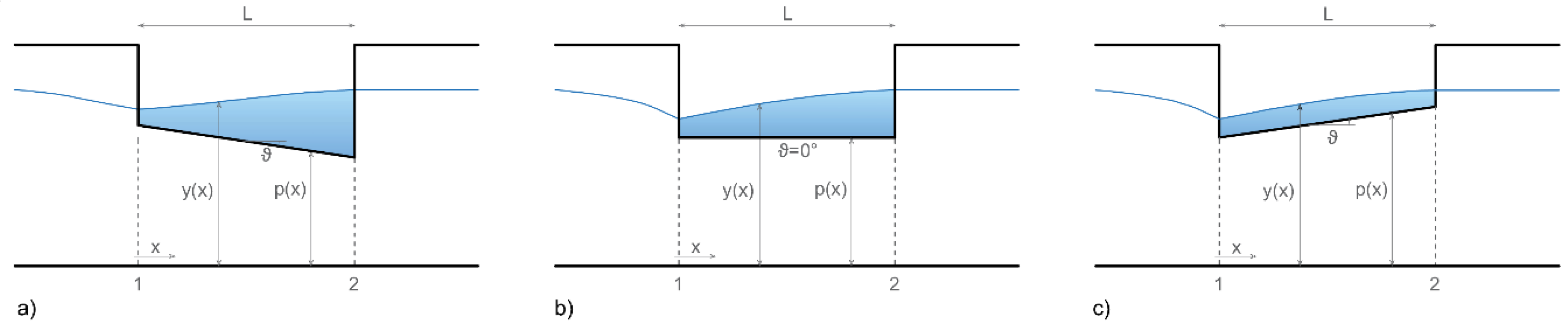
- Thirteen values of the side weir crest angle ϑ, including the horizontal case (ϑ = 0°) and upward (ϑ > 0°) or downward (ϑ < 0°) inclined configurations (ϑ = ± 1°, 2°, 3°, 4°, 6°, 9°) (Figure 1);
- Discharge coefficient C*, randomly selected in the range 0.3÷0.45 or 0.45÷0.6;
- Upstream Froude number Fr, randomly selected in the range 0.4÷0.6 or 0.6÷0.8;
- Nine values of the upstream y/p ratio, in the range 1.125÷3.25.
Furthermore, in a second step, possible changes in the energy head E were also taken into account, by adding to the previous system (18,19) the following equation:
where i and j are channel and friction slopes, respectively; j was expressed by means of the Chezy formula, as commonly used in the literature [3,23,24] and also suggested by De Marchi [1]. For these simulations considering energy variations, the following parameters were included in the analysis:
- Three values of the channel slope, i: 0.0001, 0.001 and 0.01;
- Two values of the Chezy constant χ, randomly selected in the range 20÷40 m1/2/s or 40÷60 m1/2/s.
For each combination of the selected variables, the equations were integrated until at least one of the following conditions was satisfied:
- yk = pk, i.e., the water surface profile reaches the weir crest (possible for ϑ > 0°);
- pk = 0 (possible for ϑ < 0°);
- Qd/Q1 > 0.9.
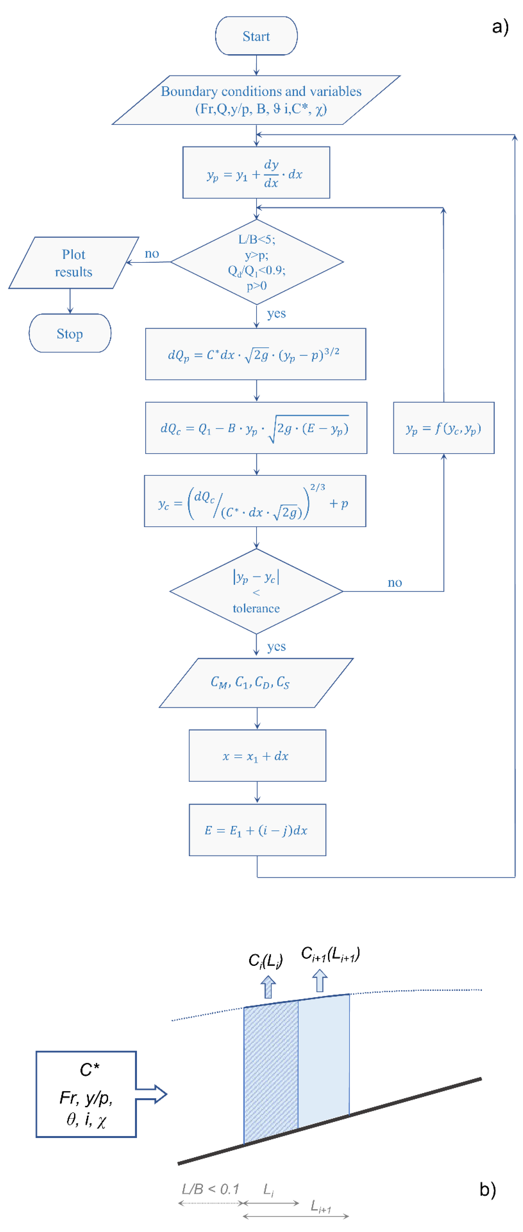
The flowchart represented in Figure 2a summarizes the implemented procedure [22]. For each integration step (dx = 2.5 mm), the first predictor yp is used for determining the diverted flow dQp with Poleni’s equation. For comparison, an additional value of the diverted flow dQc is computed as the difference between the one determined in the previous step and the one estimated with Equation (19). Then, the corrector yc is calculated as a function of Qc by inverting Poleni’s equation.
The procedure is iterated until the error in the reconstruction of each single step satisfies a prescribed tolerance of ±4‰, equal to an error in the estimation of the water surface elevation of 10−2 mm over a reference integration step of 2.5 mm. yc values for the following iterations are calculated in order to ensure the convergence of the algorithm, which is obtained using the weighted average:
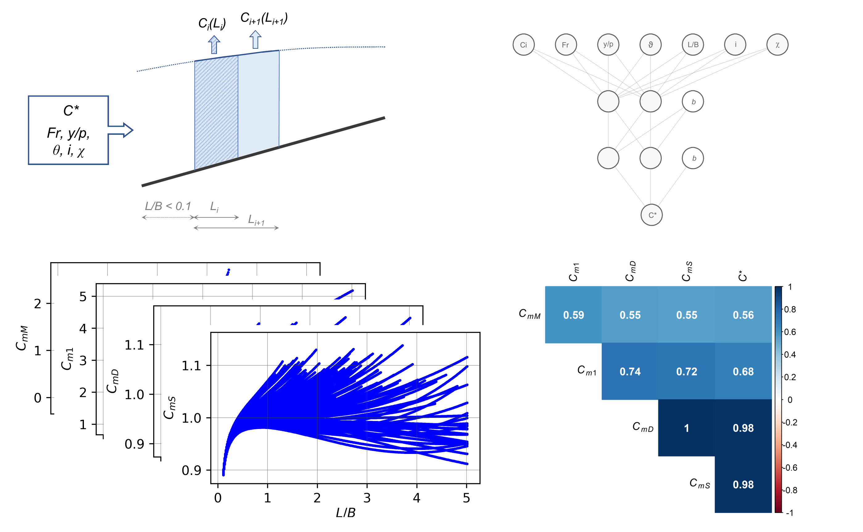
where the weight w is calculated as a function of the integration step dx, i.e., w = 1 + dx/20. For all of the different tested conditions, the discharge coefficient was evaluated over the progress of integration of the water surface profile on the side weir for each incremental step (Figure 2b), according to Equations (9), (12), (14) and (16), provided that the L/B ratio was between 0.1 and 5 (i.e., the length of the structure is physically acceptable), obtaining a total of 150,000 samples of Ci = f(C*, Fr, y/p, ϑ, L/B, i, χ) and, consequently of Cmi, based on Equation (17).
2.2. Sensitivity Analysis of Model Coefficients Cmi
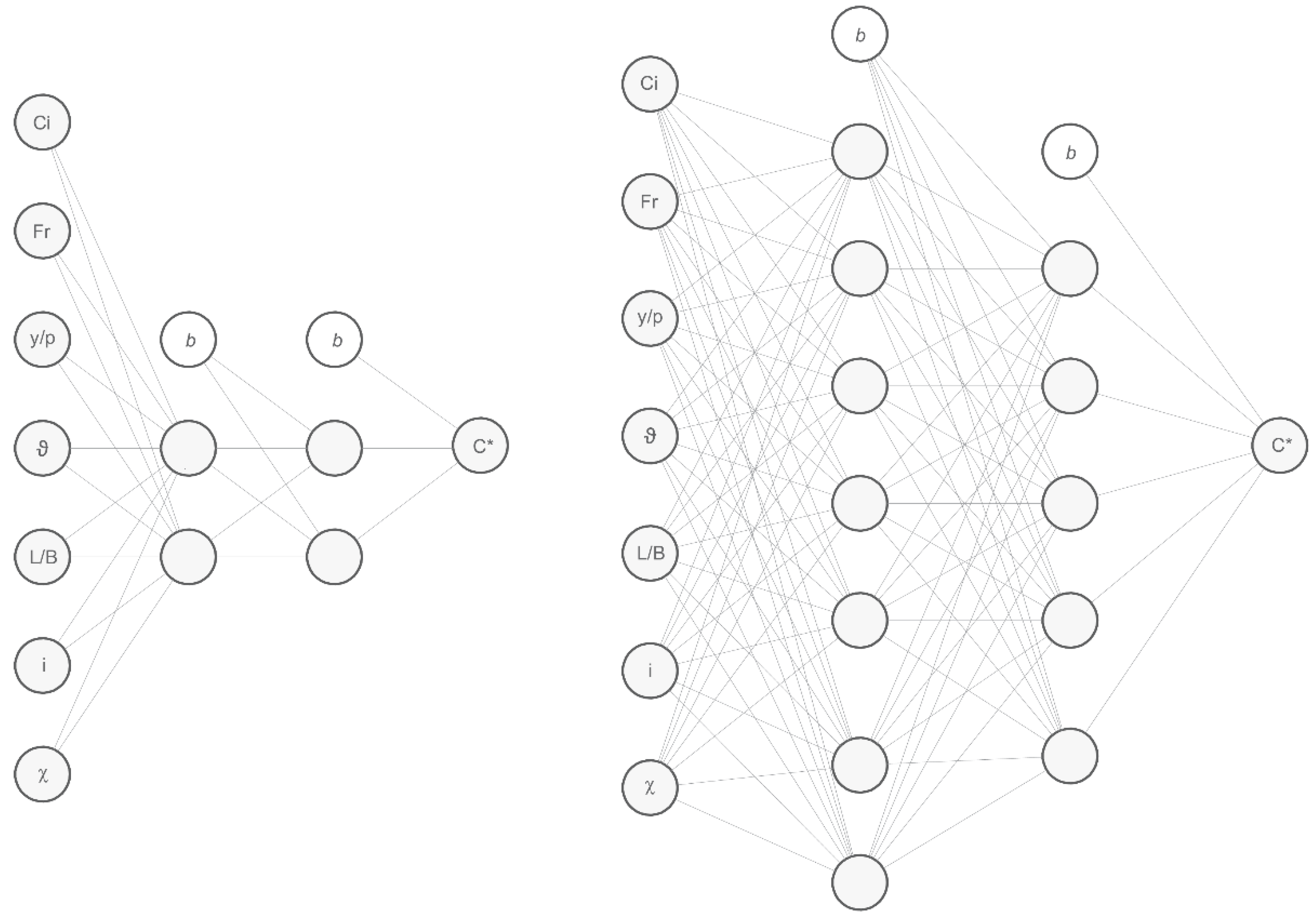
Using the synthetic datasets resulting from the numerical simulations with variable energy described in the previous section, this phase was aimed at identifying the most influencing hydraulic and geometric parameters for each model coefficient Cmi. For this purpose, in this study we implemented a multilayer perceptron, or multilayer feedforward neural network, with two hidden layers (Figure 3) and a sigmoid as an activation function, while the Levenberg–Marquardt algorithm [25] was used to train the network. The use of such networks, allowing the assessment of the functions C* = Cd = f(Ci, Fr, y/p, ϑ, L/B, i, χ), eliminates the effect of the model coefficients Cmi. Obviously, with the same approach, it is also possible to derive the functions Ci = f(C*, Fr, y/p, ϑ, L/B, i, χ), which can be combined with the previous one to “translate” discharge coefficient values originating from different modelling assumptions.
The various datasets were divided between training, testing and validation in the proportion 70-15-15, with a maximum of six validation checks. Different network sizes were tested, ranging from a minimum of two hidden layers with two neurons each (Figure 3, left) to a maximum of two layers with seven neurons on the first layer and five on the second (Figure 3, right).
All considered input parameters were reported in the representation of the architectures shown in Figure 3. However, several additional tests were performed by decreasing the number of inputs in order to analyze the sensitivity of the performances of the neural networks to the quantity and quality (i.e., type) of the input variables.
The considered minimum dataset was constituted by 38,693 elements, which excluded the risk of overfitting, given the size of implemented networks. In addition, due to the complexity of the problem, training was repeated several times for the different datasets in order to avoid the identified solution being characterized by a local minimum.
3. Results and Discussion
3.1. Effects of the Use of Oversimplified Formulas for the Experimental Assessment of the Discharge Coefficient
Figure 4 shows the obtained model coefficients Cmi as a function of the L/B ratio for the variable (left) and constant energy (right) simulations for the classical horizontal weir configurations (ϑ = 0°). The choice of visualizing the results in (L/B, Cmi) plots makes it possible to follow the trend of the calculated discharge coefficients (supposed to be constant along the side weir) over the spatial progress of each single run, for a given set of upstream boundary conditions.
As expected, the constant energy simulations provided CmM values equal to 1 (except for an essentially numerical error smaller than 0.1%), given that the solved system of Equations (18) and (19) is exactly the one at the base of De Marchi’s model. Conversely, for the C1 formula, although usually applied in the literature for assessing the discharge coefficient of horizontal weirs under the misleading definition of De Marchi′s coefficient [13,17], high values of the corresponding model coefficient Cm1 were observed. In addition, Cm1 denoted an almost linear dependence on the L/B parameter, caused by the increasing water surface elevation in the flow direction, which could partly explain the results reported by Emiroglu et al. [17], who instead attributed this behavior to the enhancement of the weir’s efficiency with its length. Instead, the values of CmD and CmS model coefficients, ranging from 0.89 to 1.15, suggest that the linear water surface profile assumption induces a relatively small error on the overall determination of the discharge coefficient. Once more, it can be noted that, for a given set of upstream conditions (i.e., following the evolution of the single run), the coefficients increase with L/B, thus indicating again a spurious dependence on this parameter, which could physically explain the results found in Emiroglu et al. [18].
When analyzing the variable energy simulations (i.e., the ones considering the effect of friction and channel slopes), no substantial differences were noted for CmD and CmS, differently from the CmM, which showed larger values up to 2. It can be observed that a reduction in the energy level can also lead to (non-physical) negative CmM values, if the energy reduction is considerable. Therefore, these results indicate that, for horizontal side weirs, CmM is more sensitive to energy variations along the structure than CmD and CmS, while it is an accurate estimator of the discharge coefficient when these changes are negligible, as is also well known in the literature [1].
For the sake of completeness, we report in the Supplement the results obtained for inclined crested geometries of the side weirs. Figure S1 clearly indicates, even more markedly than the horizontal case, high values of the Cm1, up to 15 for downward configurations (ϑ < 0°). This can be explained by considering that the C1 formula is not able to capture the increase in the pressure head in the flow direction resulting from the concurrent reduction of crest height and increase of water surface elevation when moving from upstream to downstream. Also Wang et al. [26], who analyzed the discharge coefficients for downward inclined side weirs with a physical and a numerical model, using the total head in the upstream section instead of the pressure head, observed an increase in C1 values with the crest angle. This increase was justified by them by only hydrodynamic considerations; still, we demonstrated here that the nature of this relationship is essentially geometric, as the used expression of the discharge coefficient is not influenced by the characteristics of the water surface profile. In addition, the relationship of C1 with y/p reported in [26] also seems likely to be spurious, because, for a given Fr value, a greater y/p implies a higher C1, due to the larger wetted area at an elevation higher than that of the crest in the upstream section (i.e., p1).
For upward configurations (ϑ > 0°), the Cm1 were much smaller (up to 1.6) and not always greater than 1 (Figure S2), given that while water elevation necessarily increases in the flow direction, the same cannot be said for the pressure head on the weir crest.
In contrast, with Dominguez’s and Schmidt’s approaches, we observed, in analogy with the horizontal case, smaller and more correlated model coefficients CmD and CmS, with maximum values up to 1.15 for downward geometries, ϑ < 0° (Figure S1). This result can be attributed to the concavity of the water surface profile, which was usually concave down. However, when considering the effect of friction and channel slope, it was possible to find CmD and CmS values much smaller than 1 (up to ~0.85), which can be explained by observing that, for subcritical flows and for a given value of the discharge, a reduction in the energy level is associated with a shallower water depth. This is also the reason that justifies the change in the concavity of some profiles for small L/B values, given that a large part of the energy losses generally occurs in the first part of the lateral weir. Such an effect is amplified by the increase in the diverted flow rate occurring along the structure, as a consequence of the reduction of crest height (more evident for those cases characterized by smaller y/p values in the extreme downstream section of the weir). For upward configurations (ϑ > 0°), CmD and CmS were instead characterized by larger values (in the range 0.9÷1.8 for the first and 0.9÷1.6 for the latter), more markedly for longer weirs (Figure S2), as a consequence of the more pronounced concavity of the water surface profile in the final part of the structure, due to a reduction of the derived flow rate. Therefore, even for inclined crested configurations of the side weir, the use of CD and CS expressions were found to provide reliable and correlated estimations of the discharge coefficient, even though they introduce a spurious relationship with the parameter L/B, especially for ϑ > 0°.
3.2. Sensitivity Analysis of Model Coefficients Cmi
Table 1 and Table 2 summarize the results of the analyses carried out with the use of the multilayer perceptron neural networks to identify the most influencing variables on the different model coefficients Cmi. In detail, for the selected equations for the discharge coefficient (Ci), each table reports the size of the network (first column), the number of considered parameters (the symbol X indicates whether a certain parameter has been included in the derivation of the transfer function), the average coefficient of determination (R2) between Ci and C* and the variance of R2 (σ(R2)), calculated over a minimum of four different trainings of the network, in order to avoid the problem of finding a solution characterized by a local minimum.
Table 1 indicates that with the use of CD and CS expressions it is possible to obtain satisfactory results (R2 > 0.97) even with a small network (2-2, two hidden layers with two neurons), while for C1 and CM (Table 2) it is necessary to increase the size (7-5, seven and five neurons in the first and second layer, respectively) in order to obtain acceptable R2 values. In the first case, when the number of neurons is increased, R2 approaches 1 in almost any tested condition. In addition, the results for the networks trained with CD and CS are also characterized by a small or null variance, which is indicative of the existence of a simple functional relationship. Interestingly, for CD and CS the R2 values are constantly high even when the number of the input parameters is decreased (i.e., excluding Fr, i and χ or a combination of them), while with the C1 coefficient, it is essential to include in the analysis all the selected parameters (and to use more neurons) in order to get a comparable accuracy.
The performances of the networks trained with CM (Table 2) demonstrate instead that channel slope and the Chezy roughness constant have a significant influence, even more than the Froude number, on the model coefficient values. Indeed, for the 7-5 networks, R2 values range from 0.987, calculated for those trained with all the parameters, to 0.967, when excluding only Fr, and up to 0.919 and 0.878, when excluding χ or i, respectively. In particular, Table 2 (CM, 7-5 networks) also shows an increase in the variability of the results, highlighted by larger values of the standard deviation of R2, when channel slope is not included among the input parameters. Despite this result, it is interesting to note that almost all experimental studies in the literature on the assessment of the discharge coefficient for side weirs usually neglect these parameters, relying only on the global energy constancy check, as in [15,16] (upstream vs. downstream sections of the side weir).
However, this check does not necessarily mean local energy constancy, given that a large part of the energy losses are concentrated in the initial upstream reach of the side weir, especially if the channel bed slope is not negligible.
3.3. Effects of the Use of Heterogeneous Discharge Coefficient Datasets
With a focus on classical horizontal side weirs, as depicted in Figure 4, the model coefficients Cmi have been found to be characterized by wide ranges, especially for Cm1 (1÷5) and CmM (0.1÷2.5), with the last one obviously only in the variable energy case. In addition, the correlation plot represented in Figure 5 shows very low correlation between the two coefficients and then suggests that C1 is not a good feasible alternative to the original De Marchi’s coefficient formula. Furthermore, except for CmD and CmS, the correlation coefficients reported in Figure 5 clearly indicate that the different Ci cannot be used interchangeably in the same dataset, which otherwise would not be homogeneous. This highlights the wrongness of building datasets for deriving predictive formulas or for verifying their goodness with experimental discharge coefficient data coming from different modelling approaches. As shown in the Supplement, this result was also found to be valid (even more markedly) for inclined configurations of the side weir.
This may appear obvious, but, as mentioned in the Introduction, examples of these cases still exist in the literature: for example, Shariq et al. [14] obtained an empirical formula for CD, but they evaluated its performance by comparing its predicting ability to that of other equations that are not based on Dominguez’s approach; Parsaie and Haghiabi [20] used machine learning algorithms to predict the discharge coefficient based on an ensemble experimental dataset comprising C1, CD and CM values and compared the results with those obtained by applying other empirical formulas from the literature; similarly, Ebtehaj et al. [21] developed a predictive model based on data coming from Emiroglu et al. [17] and Bagheri et al. [13], who expressed the discharge coefficient in terms of C1 and CD, respectively.
A possible solution to this heterogeneity issue could be achieved by using the neural networks introduced in Section 2.2. Indeed, by eliminating the effect of the assumption on the shape of the water surface profile (i.e., the effect of Cmi), they can act as “homogenization functions” in two possible ways: (i) to obtain an homogeneous C* = Cd dataset starting from differently computed Ci, or (ii) to transform a dataset of different Ci into an homogeneous Ci dataset (e.g., a mixed CD and C1 dataset to a single CS dataset). The first solution allows to deduce more reliable information about the overflow efficiency, while the second makes it possible to compare discharge coefficient equations which are experimentally derived using different modelling approaches.
4. Conclusions
The idea of this study originated from the necessity of critically discussing the following aspects regarding the assessment of the discharge coefficient of side weirs: (i) the effects of the use of oversimplified formulas for the experimental determination of the discharge coefficients; (ii) the error associated with the use of heterogeneous discharge coefficient datasets, i.e., obtained with models based on different assumptions on the shape of the water surface profile over the side weir; (iii) the influence of the different input parameters on each considered model coefficient Cm, which is the responsible for possible misinterpretations of the efficiency of side weirs.
The results revealed a first interesting insight: despite being used interchangeably in the literature under the common definition of “De Marchi’s formula”, C1 and CM were found to have extremely different values of the corresponding model coefficients Cm1 and CmM, with very low correlation. CmD and CmS were instead highly correlated among them, given that they rely on similar hypotheses on the shape of the water surface profile, and then they could be used interchangeably, as also experimentally shown by [18].
The identified large ranges of the model coefficient values should also warn on possible misleading information provided by the Ci coefficients on the overflow efficiency of side weirs. Indeed, the identified variability of Cmi is comparable to one of the corresponding Ci values usually described in the literature [13,16,17,18]. Moreover, the model coefficients showed different sensitivity to the input hydraulic and geometric parameters. In particular, we observed that L/B strongly affects the Cm1 values, meaning that the correlation identified in the literature [17,18], between C1 and L/B, should not necessarily be intended as an overflow efficiency improvement, but merely as a spurious dependence. Interesting results were also provided by the sensitivity analysis of the De Marchi’s model coefficient CmM, demonstrating an important role of channel slope and Chezy’s roughness, despite usually being neglected in experimental equations for the assessment of the discharge coefficient. However, it is important to stress that the results of this last point on CM refer only to the influence of the constant-energy hypothesis, while a further experimental analysis would be required for a global assessment of the De Marchi’s model for the side weirs.
Overall, the results clearly demonstrated the wrongness of using or building non homogeneous datasets of Ci (i.e., coming from different modelling approaches) to obtain and/or compare predictive experimental discharge coefficient formulas. Nonetheless, it was shown that no reliable considerations on the overflow efficiency can be inferred from the analysis of Ci values, unless the effect of Cmi is properly accounted for.
In this study, we then proposed the use of neural networks as a solution to the two highlighted issues. Indeed, the functions C* = f(Ci, Fr, y/p, ϑ, L/B, i, χ) eliminate the effect of the model coefficients Cmi, then allowing a more reliable evaluation of the overflow efficiency. In a second step, combining the previous functions with Ci = f(Ci*, Fr, y/p, ϑ, L/B, i, χ), it would be possible to “translate” discharge coefficient values originating from different models to create homogenous datasets.
Supplementary Materials
The following are available online at https://www.mdpi.com/2073-4441/11/12/2585/s1, Figure S1: Analysis of obtained model coefficients Cmi for downward inclined side weirs: variable energy (left) and constant energy (right) simulations; Figure S2: Analysis of obtained model coefficients Cmi for upward inclined side weirs: variable energy (left) and constant energy (right) simulations.
Author Contributions
Conceptualization, M.D.B. and A.R.S.; methodology, M.D.B. and A.R.S.; investigation, M.D.B.; visualization, M.D.B. and A.R.S.; writing—original draft preparation, A.R.S.; writing—review and editing, M.D.B. and A.R.S.
Funding
This research received no external funding.
Conflicts of Interest
The authors declare no conflict of interest.
References
- De Marchi, G. Saggio di teoria del funzionamento degli stramazzi laterali. L. Energ. Elettr. 1934, 11, 849–860. (In Italian) [Google Scholar]
- Subramanya, K.; Awasthy, S. Spatially varied flow over side weirs. J. Hydraul. Div. 1972, 98, 1–10. [Google Scholar]
- Singh, R.; Manivannan, D.; Satyanarayana, T. Discharge coefficient of rectangular side weirs. J. Irrig. Drain. Eng. 1994, 120, 814–819. [Google Scholar] [CrossRef]
- El-Khashab, A.; Smith, K.V. Experimental investigation of flow over side weirs. J. Hydraul. Div. 1976, 102, 1255–1268. [Google Scholar]
- Ranga Raju, K.; Prasad, B.; Gupta, S.K. Side weir in rectangular channel. J. Hydraul. Div. 1979, 105, 547–554. [Google Scholar]
- Hager, W. Lateral outflow over side weirs. J. Hydraul. Eng. 1987, 113, 491–504. [Google Scholar] [CrossRef] [Green Version]
- Uyumaz, A.; Smith, R.H. Design procedure for flow over side weirs. J. Irrig. Drain. Eng. 1991, 117, 79–90. [Google Scholar] [CrossRef]
- Swamee, P.K.; Pathak, S.K.; Ali, M.S. Side-weir analysis using elementary discharge coefficient. J. Irrig. Drain. Eng. 1994, 120, 742–755. [Google Scholar] [CrossRef]
- Muslu, Y. Numerical analysis of lateral weir flow. J. Irrig. Drain. Eng. 2001, 127, 246–253. [Google Scholar] [CrossRef]
- Michelazzo, G. New analytical formulation of De Marchi model for a zero-height side weir. J. Hydraul. Eng. 2015, 141, 04015030. [Google Scholar] [CrossRef]
- Dominguez, F.J. Curso de Hidráulica; Nascimento: Santiago, Chile, 1935. (In Spanish) [Google Scholar]
- Schmidt, M. Zur Frage des Abflusses Uber Streichwehre: Eine Kritische Betrachtung der Bekanntesten Berechnungsverfahren und Versuche im Zusammenhang mit Eigenen Versuchen; Technische Universitat Charlottenburg: Berlin, Germany, 1954. (In German) [Google Scholar]
- Bagheri, S.; Kabiri-Samani, A.; Heidarpour, M. Discharge coefficient of rectangular sharp-crested side weirs -part I: Traditional weir equation. Flow Meas. Instrum. 2014, 35, 109–115. [Google Scholar] [CrossRef]
- Shariq, A.; Hussain, A.; Ansari, M.A. Lateral flow through the sharp crested side rectangular weirs in open channels. Flow Meas. Instrum. 2018, 59, 8–17. [Google Scholar] [CrossRef]
- Mohammed, M.Y.; Mohammed, A.Y. Discharge coefficient for an inclined side weir crest using a constant energy approach. Flow Meas. Instrum. 2011, 22, 495–499. [Google Scholar] [CrossRef]
- Bagheri, S.; Kabiri-Samani, A.; Heidarpour, M. Discharge coefficient of rectangular sharp-crested side weirs -part II: Domínguez’s method. Flow Meas. Instrum. 2014, 35, 116–121. [Google Scholar] [CrossRef]
- Emiroglu, M.E.; Agaccioglu, H.; Kaya, N. Discharging capacity of rectangular side weirs in straight open channels. Flow Meas. Instrum. 2011, 22, 319–330. [Google Scholar] [CrossRef]
- Emiroglu, M.; Ikinciogullari, E. Determination of discharge capacity of rectangular side weirs using Schmidt approach. Flow Meas. Instrum. 2016, 50, 158–168. [Google Scholar] [CrossRef]
- Vatankhah, A.R.; Velayati, F.; Azimi, M. Discussion of “Discharge Characteristics of a Trapezoidal Labyrinth Side Weir with One and Two Cycles in Subcritical Flow” by M.E. Emiroglu, M.C. Aydin and N. Kaya. J. Irrig. Drain. Eng. 2015, 141, 07015003. [Google Scholar] [CrossRef]
- Parsaie, A.; Haghiabi, A. The effect of predicting discharge coefficient by neural network on increasing the numerical modeling accuracy of flow over side weir. Water Resour. Manag. 2015, 29, 973–985. [Google Scholar] [CrossRef]
- Ebtehaj, I.; Bonakdari, H.; Gharabaghi, B. Development of more accurate discharge coefficient prediction equations for rectangular side weirs using adaptive neuro-fuzzy inference system and generalized group method of data handling. Measurement 2018, 116, 473–482. [Google Scholar] [CrossRef]
- Di Bacco, M.; Scorzini, A.R.; Leopardi, M. On the experimental assessment of De Marchi’s discharge coefficient for inclined side weirs: Transfer functions for the application of alternative methods. In Proceedings of the 38th IAHR World Congress, Panama City, Panama, 1–6 September 2019. [Google Scholar] [CrossRef]
- Ghodsian, M. Supercritical flow over a rectangular side weir. Can. J. Civil. Eng. 2003, 30, 596–600. [Google Scholar] [CrossRef]
- Aghayari, F.; Honar, T.; Keshavarzi, A. A study of spatial variation of discharge coefficient in broad-crested inclined side weirs. Irrig. Drain. 2009, 58, 246–254. [Google Scholar] [CrossRef]
- Marquardt, D.W. An algorithm for least-squares estimation of nonlinear parameters. J. Soc. Ind. Appl. Math. 1963, 11, 431–441. [Google Scholar] [CrossRef]
- Wang, Y.; Wang, W.; Hu, X.; Liu, F. Experimental and numerical research on trapezoidal sharp-crested side weirs. Flow Meas. Instrum. 2018, 64, 83–89. [Google Scholar] [CrossRef]
Figure 1.
Schematization of side weir configurations: (a) inclined downward; (b) horizontal; (c) inclined upward. y(x) and p(x) indicate the water surface and weir’s crest profile; ϑ is the crest angle.
Figure 1.
Schematization of side weir configurations: (a) inclined downward; (b) horizontal; (c) inclined upward. y(x) and p(x) indicate the water surface and weir’s crest profile; ϑ is the crest angle.

Figure 2.
Schematization of the implemented procedure: (a) flowchart of the predictor–corrector method; (b) integration of the water surface profile: input and output variables.
Figure 2.
Schematization of the implemented procedure: (a) flowchart of the predictor–corrector method; (b) integration of the water surface profile: input and output variables.

Figure 3.
Architecture of implemented neural networks: considered minimum (left) and maximum (right) number of neurons per hidden layer (in each network, the input layer is represented on the left, the output layer on the right; b indicates the bias in the hidden layers).
Figure 3.
Architecture of implemented neural networks: considered minimum (left) and maximum (right) number of neurons per hidden layer (in each network, the input layer is represented on the left, the output layer on the right; b indicates the bias in the hidden layers).

Figure 4.
Analysis of obtained model coefficients Cmi for horizontal side weirs: variable energy (left) and constant energy (right) simulations.
Figure 4.
Analysis of obtained model coefficients Cmi for horizontal side weirs: variable energy (left) and constant energy (right) simulations.

Figure 5.
Correlation plot of model coefficients for horizontal side weir configuration.


Table 1.
Results of the analysis of the transfer functions from CD and CS: sensitivity to network size and input parameters.
Table 1.
Results of the analysis of the transfer functions from CD and CS: sensitivity to network size and input parameters.
| Neurons (I, II Layer) | Parameters | CD | CS | |||||||
|---|---|---|---|---|---|---|---|---|---|---|
| Fr | y/p | L/B | ϑ | i | χ | R2 | σ(R2) | R2 | σ(R2) | |
| 2, 2 | x | x | x | x | x | 0.973 | 0.003 | 0.978 | 0.010 | |
| x | x | x | x | 0.975 | 0.003 | 0.975 | 0.009 | |||
| x | x | x | x | x | x | 0.976 | 0.003 | 0.977 | 0.009 | |
| x | x | x | x | x | 0.976 | 0.002 | 0.978 | 0.010 | ||
| x | x | x | x | 0.972 | 0.005 | 0.972 | 0.010 | |||
| x | x | x | x | 0.971 | 0.004 | 0.973 | 0.010 | |||
| x | x | x | x | x | 0.972 | 0.005 | 0.972 | 0.009 | ||
| 7, 5 | x | x | x | x | x | 0.998 | 0.000 | 0.994 | 0.000 | |
| x | x | x | x | 0.997 | 0.000 | 0.993 | 0.000 | |||
| x | x | x | x | x | x | 0.999 | 0.000 | 0.995 | 0.000 | |
| x | x | x | x | x | 0.997 | 0.000 | 0.994 | 0.000 | ||
| x | x | x | x | 0.993 | 0.000 | 0.990 | 0.000 | |||
| x | x | x | x | 0.993 | 0.000 | 0.991 | 0.000 | |||
| x | x | x | x | x | 0.993 | 0.000 | 0.992 | 0.000 | ||
Table 2.
Results of the analysis of the transfer functions from C1 and CM: sensitivity to network size and input parameters.
Table 2.
Results of the analysis of the transfer functions from C1 and CM: sensitivity to network size and input parameters.
| Neurons (I, II Layer) | Parameters | C1 | CM | |||||||
|---|---|---|---|---|---|---|---|---|---|---|
| Fr | y/p | L/B | ϑ | i | χ | R2 | σ(R2) | R2 | σ(R2) | |
| 2, 2 | x | x | x | x | x | 0.597 | 0.013 | 0.639 | 0.019 | |
| x | x | x | x | 0.597 | 0.014 | 0.541 | 0.029 | |||
| x | x | x | x | x | x | 0.608 | 0.009 | 0.822 | 0.029 | |
| x | x | x | x | x | 0.606 | 0.010 | 0.716 | 0.015 | ||
| x | x | x | x | 0.569 | 0.010 | 0.649 | 0.040 | |||
| x | x | x | x | 0.580 | 0.001 | 0.715 | 0.023 | |||
| x | x | x | x | x | 0.572 | 0.013 | 0.791 | 0.027 | ||
| 7, 5 | x | x | x | x | x | 0.931 | 0.006 | 0.878 | 0.012 | |
| x | x | x | x | 0.915 | 0.005 | 0.731 | 0.116 | |||
| x | x | x | x | x | x | 0.962 | 0.007 | 0.987 | 0.008 | |
| x | x | x | x | x | 0.942 | 0.006 | 0.919 | 0.006 | ||
| x | x | x | x | 0.856 | 0.003 | 0.826 | 0.055 | |||
| x | x | x | x | 0.876 | 0.003 | 0.874 | 0.020 | |||
| x | x | x | x | x | 0.884 | 0.008 | 0.967 | 0.008 | ||
© 2019 by the authors. Licensee MDPI, Basel, Switzerland. This article is an open access article distributed under the terms and conditions of the Creative Commons Attribution (CC BY) license (http://creativecommons.org/licenses/by/4.0/).
Share and Cite
MDPI and ACS Style
Di Bacco, M.; Scorzini, A.R. Are We Correctly Using Discharge Coefficients for Side Weirs? Insights from a Numerical Investigation. Water 2019, 11, 2585. https://doi.org/10.3390/w11122585
AMA Style
Di Bacco M, Scorzini AR. Are We Correctly Using Discharge Coefficients for Side Weirs? Insights from a Numerical Investigation. Water. 2019; 11(12):2585. https://doi.org/10.3390/w11122585
Chicago/Turabian StyleDi Bacco, Mario, and Anna Rita Scorzini. 2019. "Are We Correctly Using Discharge Coefficients for Side Weirs? Insights from a Numerical Investigation" Water 11, no. 12: 2585. https://doi.org/10.3390/w11122585
Note that from the first issue of 2016, this journal uses article numbers instead of page numbers. See further details here.