Intratidal Variability of Water Quality in the Damariscotta River, Maine


Department of Civil and Environmental Engineering, University of Maine, 5711 Boardman Hall, Orono, ME 04469, USA
*
Author to whom correspondence should be addressed.
Water 2019, 11(12), 2603; https://doi.org/10.3390/w11122603
Submission received: 31 October 2019
/
Revised: 3 December 2019
/
Accepted: 5 December 2019
/
Published: 10 December 2019
(This article belongs to the Section Water Quality and Contamination)
Abstract
:The Damariscotta River Estuary in midcoast Maine, which houses over forty hectares of American oyster aquaculture, is characterized by several bathymetric sills, constrictions, and headlands. The geography, hydrology, and biochemistry of the estuary are closely intertwined, as its irregular shape contributes to spatially varying patterns of tidal flow, which are in turn responsible for sediment suspension. This project explores the spatial and temporal variability of the water level and current cycles of the estuary and how they are correlated to measures of water quality, such as turbidity, salinity, pH, and oxygen concentration. From July to November 2016, absolute pressure data from twelve sites were collected along the river, from which a tidal elevation time series was computed. In addition, velocity current profiles, water quality data, and wind data were obtained from surface buoys, and transects were collected in three major regions along the river. The lower and mid reaches of the estuary have a vertical shear structure of tidal flow, as high salinity water enters the estuary along the bottom during flood phase, is uplifted during the slack period, and flushed out at the surface during ebb phase. In this region, overtides are relatively weak compared to upstream, dissipation near the bottom is minimal, and turbidity and chlorophyll oscillate out of phase. North of the Glidden Ledges constriction, a headland causes the shear structure to become lateral, where dissipation is elevated during the flood phase throughout the entire water column. Dissipation has a quarter-diurnal harmonic due to increased turbulence during peak ebb and peak flood, which results in disproportionately high intratidal amplitudes in turbidity and chlorophyll. Overall, the bathymetry and tidal patterns of the estuary help to explain why the upper reaches tend to be more viable for shellfish aquaculture.
1. Introduction
The Damariscotta River Estuary is home to over 40 hectares of aquaculture, primarily American oyster, along with blue mussel, scallops, and seaweed [1]. The river produces the majority of Maine’s oysters, between one million and three million units per year, and has a financial impact of millions of dollars each year [2]. The Damariscotta River features archaeological evidence of the negative impacts of climate change on shellfish. Oyster middens are mounds of human-disposed oyster shells, which line the edges of the river near Newcastle and Damariscotta and were formed from 200 BC to 1000 AD [3]. At the time the middens were discovered, there was an absence of oysters in the region. Increasing salinities and corresponding predators (oyster drill) and diseases (dermo and vibrio) were introduced to the system via climate change effects, leading to the extinction of the local oyster population, which has since rebounded. The Gulf of Maine waters are warming faster than 99% of the world’s ocean [4], which can impact water quality and wave climates [5]. Due to the direct and indirect effects of climate change on the aquaculture industry, there is considerable economic interest in understanding how hydrodynamics influence various parameters relevant to oyster growth, including turbidity, pH, salinity, and chlorophyll concentration.
Previous research into the Damariscotta estuary explored the unique features of the headland located north of a constricted sill at Glidden Ledges, and its effects on tidal dynamics [6]. A gyre forms upstream of the headland during the flood phase, which enhances inland flow over the eastern channel and is countered by seaward flow over the western shoals. This gyre results in opposing lateral shear structures in velocity that flow over each other, thus creating a vertical shear structure. Because of these secondary flows, tidal and intratidal patterns of lateral advection and stress divergence emerge. Lateral advection effects tend to dominate the dynamics near the surface, and bottom friction effect forces dominate at the bottom during neap tide and throughout the water column during spring tide. Recent research has also shown that floating oyster farms in the upper reach of the estuary induce surface friction effects that reduce flow through the region, influencing fluid momentum across the estuary [7].
Long-term transport of particles relevant to oyster aquaculture in tidally-driven converging estuaries is dominated by the tidal characteristics of the system. As the tide interacts with the surrounding bathymetry, several nonlinear forcing mechanisms such as advection and bottom friction interact with the dominant tide to create irregular high frequency overtides [8]. These barotropic overtides tend to be an order of magnitude smaller in water level amplitude than the dominant tidal harmonics, but their along-channel velocities can be quite significant and therefore impact long-term material transport [9]. These effects are compounded by constrictions which may either amplify or attenuate tidal energy flux depending on the shape of the constrictions and the composition of the river bed [10].
Previous research into the effects of tidal asymmetry, including flood–ebb difference in tidal amplitude and in duration on water quality has mostly pertained to sediment transport and salinity. Seasonal variation in semidiurnal and quarter-diurnal (M2 and M4) tidal phases can result in similar variation in material transport, and sediment flux may vary by 10% to 50% per year [11]. Sediment flux may also be influenced by tidal reflection off dams or constrictions. In estuaries with low river flows, suspended particulate matter originates from resuspension by tidal shear stresses acting on the riverbed [12].
Dissipation of kinetic energy plays an important role in the distribution of sediment in the estuary. Turbulent kinetic energy (TKE) production can be estimated as a product of the Reynolds stresses and the velocity shear [13]. According to Simpson et al. [14], TKE production is cubically related to the depth-mean tidal current speed and oscillates at double the frequency of the dominant tidal harmonic; therefore, semidiurnal tidal frequencies result in quarter-diurnal dissipation frequencies.
It has long been established that the patterns of tidal and subtidal flow in an estuary contribute to regions of estuary turbidity maxima, which can store up to a year of an estuary’s supply of sediment [15]. Phase differences between current velocity and suspended sediment caused by flood–ebb tidal velocity asymmetry can contribute to the residual fluxes of sediment [16]. Reynolds stresses in the flow alongside vertical velocity shear give rise to elevated rates of production of turbulent kinetic energy, which causes sediment to be lifted from the estuarine bottom [17]. Tidal patterns of sediment are correlated with tidal patterns in other water quality metrics, as sediment porewater has lower pH and oxygen than fresh river water [18]. In addition, since sediment inhibits sunlight and the development of phytoplankton, a link can be drawn between turbulence and chlorophyll measurements [19].
Research into correlations between tidal harmonics and other water quality parameters has been limited. In a coupled hydrodynamic and biochemical model, it was shown that phytoplankton bloom rates are dependent on the relative time scales of plankton growth and advection [20]. Blooms tend to flourish when freshwater discharge rates are low; however, some advection is necessary to ensure delivery of nutrients. Excess flow viscosity, which is inherently linked to dissipation, results in the production of sea foam which enhances chlorophyll production [19]. This may imply that dissipation and chlorophyll concentration operate on the same harmonic scale but out of phase.
Although there is considerable research into how tidal harmonics affect tidal asymmetry and thus material transport, there has been little research into how tidal patterns affect water quality on temporal scales. Metrics such as turbidity, salinity, and chlorophyll are generally researched through a spatial lens, or a long-term temporal lens, in terms of transport distances and subtidal flow. For example, longer estuaries tend to have greater concentrations of suspended particulate matter than shorter estuaries, due to their longer flushing times [21]. Longer flushing times may contribute to increased development of plankton and bacteria, as there is more opportunity for nutrients to be absorbed [22]. Climate change may play a role in algae production in estuaries, as irregular cycles of rainfall during the wet season followed by drought during the dry season can cause a cycle of increased inflow of nutrients followed by long residence times [23].
It is well known that waste products inherent in finfish aquaculture contribute to algae blooms on a variety of spatial and temporal scales [24]. However, a recent study concluded that there is no correlation between oyster aquaculture and the biomass of Zostera marina, but they may have an effect on the biome of organizations that live on seagrass [25]. In addition, the management and maintenance of aquaculture structures may significantly increase sediment concentrations within the water column [26].
This project asks how the geometry of a tidally driven estuary affects patterns of asymmetries and irregularities in tidal flow. The objectives of this work are to characterize the tidal behavior of this system, demonstrate how tides influence water quality, and describe their spatial variability. In a complex estuary like the Damariscotta River, an improved understanding of intratidal patterns may help to inform aquaculture siting, long-term trends, and the potential effects of climate change on aquaculture viability. First, the paper discusses the tidal dynamics of the estuary and describes how as the estuary converges, the diurnal and semidiurnal amplitudes remain steady, while the overtidal constituents are amplified. Next, transect data at three sites are utilized to explain how the varying bathymetry along the estuary results in tidal and quarter-diurnal patterns of TKE dissipation, and how dissipation is linked to increased turbidity primarily if the region of elevated dissipation extends to the estuarine bottom. The inverse link between turbidity and chlorophyll is also analyzed. Finally, the paper discusses the direct temporal correlation between the tidal harmonics of along-channel current velocity and the related harmonics of turbidity, salinity, chlorophyll, and pH.
Study Area
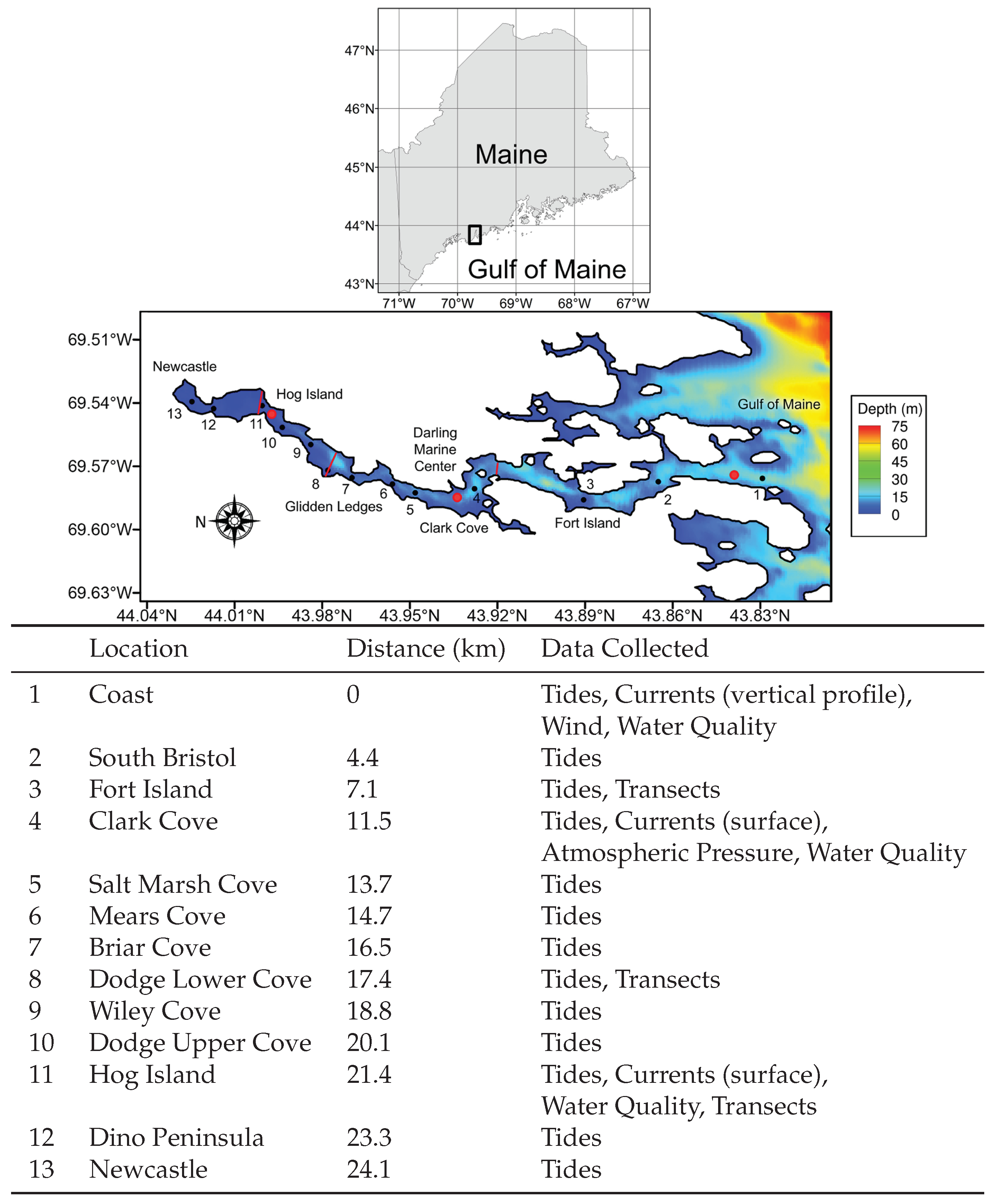
The Damariscotta River is a mesotidal glacially carved estuary in midcoast Maine with very little freshwater input (Figure 1). The estuary originates in Damariscotta Lake near the town of Newcastle and flows 30 km southward, draining into the Gulf of Maine (Figure 1). The estuary is generally convergent, with a width of 975 m at the mouth and 45 m at the head. The Damariscotta river is relatively short (wave number × estuary length ) and semidiurnally dominant (form factor = (diurnal amplitudes)/(semidiurnal amplitudes) = 0.142), with low discharge rates. Freshwater input is governed by the operation of Damariscotta Lake Dam, with a discharge ranging from 0.1 to 12 /s in 2016, with a wet season in the spring and a dry season in the summer and fall. Tidal ranges vary from 2.2 to 3.6 m from neap and spring tide at the mouth, respectively, and average annual precipitation is ∼1200 mm of rainfall and ∼1750 mm of snowfall [27]. Monthly precipitation ranges from ∼80 mm per month in the dry season to ∼120 mm per month in the wet season. Snowfall typically begins in late November and ends in early April, with the highest rates of ∼350 mm per month in January and February.
Multibeam bathymetry data shows that bedrock constrictions and sill morphology resulted in uneven distributions of sediment throughout the Holocene epoch [28]. Shipp et al. [29] identified eight sills or constrictions that define seven basins along with Salt Bay, which lies at the end of the estuary, but there are three significant constrictions that divide Damariscotta River geographically and dynamically into four primary regions. Fort Island, located 7.1 km landward of the coast, occupies about 75% of the cross-sectional area and is considered by [30] to be the official starting point of the estuary. Mid range in Damariscotta river lies Clark Cove, a right-angle bend in the river that is home to the Darling Marine Center and several aquaculture farms. Finally, Glidden Ledges is a 200 m wide constriction in the northern reach, which is characterized by large quantities of stored sediment and intertidal flats bounding a thalweg (Figure 1). Although the most sediment is stored in the northern region, the thickest sediment layers lie in isolated deposits in the middle and southern regions; however, around the Clark Cove constriction, much of the riverbed is exposed bedrock. The region of Damariscotta River between Fort Island and Clark Cove, the region between Clark Cove and Glidden Ledges, and the region north of Glidden Ledges are referred to as the southern, central, and northern reaches, respectively. Buoy and satellite derived data of chlorophyll-a, water temperature, and turbidity demonstrate that the northern reaches of the estuary are especially suitable for oyster aquaculture [31]. The high concentration of chlorophyll-a in the northern reaches is due in part to the high degree of light penetration in the area, reaching down to the benthic layer [32].
2. Materials and Methods
2.1. Data Collection
This project compiles data from a variety of sources and consolidates them into a single overview of the tidal and water quality dynamics of the Damariscotta River. Water level data were collected along 13 sites from 12 July to 12 November of 2016 using HOBO (Honest Observer by Onset) U20L Water Level Loggers moored to the river bottom by concrete anchors (Figure 1), with one additional logger deployed in air near Clark Cove to measure barometric pressure. Total elevation levels were computed at 1 min intervals from the difference between absolute and barometric pressures, divided by the density of water. Current velocities at a single point below the surface, as well as several water quality metrics such as turbidity, salinity, temperature, pH, and chlorophyll, were collected at one-hour intervals from two Sea-Bird LOBO (Land/Ocean Biogeochemical Observatory) buoys. They were deployed one meter below the surface in the center of the channel near Clark Cove and Hog Island, and they were maintained by the Sustainable Ecological Aquaculture Network (SEANET) from September 2015 to November 2016. A third buoy was deployed at the coast and measured a vertical profile of current velocity in two meter bin intervals and twenty min time intervals via a RDI WHS-600 kHz Acoustic Doppler Current Profiler (ADCP). The buoy also collected wind data at ten min intervals three meters above the surface via a Gill Instruments WindSonic Ultrasonic Wind Sensor. In addition, temperature and conductivity data were collected in five meter bins and twenty min time intervals via a Sea Bird Electronics MicroCAT (Computerized Axial Tomography) C-T (conductivity, temperature) recorder, from which water salinity and density were computed.
In order to get a more detailed perspective of spatial estuarine flow patterns along the estuary, lateral transect measurements were collected during spring and neap tide near Glidden Ledges on 29 April (spring) and 14 May (neap), 2017, near Clark Cove on 30 April (spring) and 13 May (neap), 2017, and near Hog Island on 17 June (neap) and 23 June (spring), 2017 (Figure 1). For each field day, a vessel towed 1200 kHz Acoustic Doppler Current Profiler (ADCP) and Rockland Scientific MicroCTD (conductivity, temperature, depth) were deployed near Dodge Lower Cove, just north of the Glidden Ledges constriction, to collect cross-channel transect data in roughly 30 min intervals for approximately 13 h. The ADCP was mounted in a trimaran, towed along-side another vessel traveling at 1.5–2 m/s and collected east–west and north–south current velocities throughout the cross-section in 0.5 m vertical bins. Concurrently, the MicroCTD collected density and turbidity data at four stations across the river. The MicroCTD was equipped with a pressure sensor, temperature and conductivity probes, turbidity and chlorophyll sensors, and 2 shear probes. For this study, the MicroCTD was used in descending mode in the middle reach and ascending mode in the upper reach, effectively creating vertical profiles ranging ∼1.5–2 m below the water surface to 1 m above the bottom. Between five and seven profiles were collected over a 10 min period and averaged to account for intermittency in turbulence measurements. It is important to note that discharge rates of the Damariscotta Estuary are much higher during the wet season than during the dry season, when the data near Glidden Ledges was collected (∼6 compared to ∼0.2 ). Comparisons between LOBO data, ADCP data, and CTD data are only made at similar times of year, with similar forcing conditions.
Bathymetry data for the Damariscotta River was compiled from Chandler [28] and data for the Gulf of Maine are courtesy of the National Geophysical Data Center. The bathymetry data were merged through Kriging interpolation, which ensures the distribution of water depths is unchanged by the interpolation algorithm [33].
2.2. Data Processing
Water levels were computed from pressure data, and water density was computed from salinity and temperature. Erroneous data were removed manually, and the water levels were detrended so that the time series at each station has a zero mean and no linear trend. Tidal constituents were computed with the t_tide MATLAB script, which uses a modified least squares fit method to compute amplitudes and phases [34]. Since only the tidal elevation data were captured at a small enough time interval to distinguish between overtides of the same species, when discussing current, water quality, or transect data, the semidiurnal, quarter-diurnal, and sixth-diurnal tidal species are referred to as D2, D4, and D6 respectively, following Jay and Kukulka [35]. These three tidal species are mainly composed of the M2, M4, and M6 tidal constituents, respectively.
East–west and north–south velocities were rotated to reflect along and across channel velocities, postprocessed to eliminate error, and interpolated onto a uniform grid. The along channel and across channel velocity are defined as u and v, respectively, on a y-z (across channel-depth) axis in several time slices. Turbulence and dissipation data were processed as per Lieberthal et al. [6].
The power spectral density (PSD) of a discrete time series represents the power of the frequency component’s contribution to the signal, which is estimated for a finite, discrete series via a periodogram, with a hanning window of size 4. The PSD, represented by the variable S, is given for the tides, currents, and water quality metrics in the Discussion section. The PSD analysis is used to show the frequency distribution of power within each time series, and how certain tidal constituents emerge in the data that may not be obvious otherwise [36].
3. Results
3.1. Tidal Characterization
Table 1 shows the tidal species of water elevation and surface current at the coast, Clark Cove, and Hog Island. At the coast, the tides were measured to be flood–ebb symmetric in duration, and the tidal amplitude ranged from 1.1 to 1.8 m during neap and spring tide, respectively. The surface current at the coast featured a semidiurnal amplitude of 0.11 m/s in neap tide and 0.22 m/s in spring tide. Unlike in tidal elevation, the quarter-diurnal (D4) component of the surface current was not negligible, at about 11% the amplitude of the semidiurnal (D2) component. Hog Island had similar D2, D4, and sixth-diurnal (D6) current amplitudes as at the coast, but the current was reduced at Clark Cove. The D2 amplitude of current velocity at Clark Cove was just 0.18 m/s, and the D4 amplitude was one third of that at the coast and Hog Island. The diurnal amplitude was actually highest in the northern reach (due to the Glidden Ledges constriction), the semimonthly amplitude was uniform throughout the estuary, and the monthly amplitude diminishes upstream.
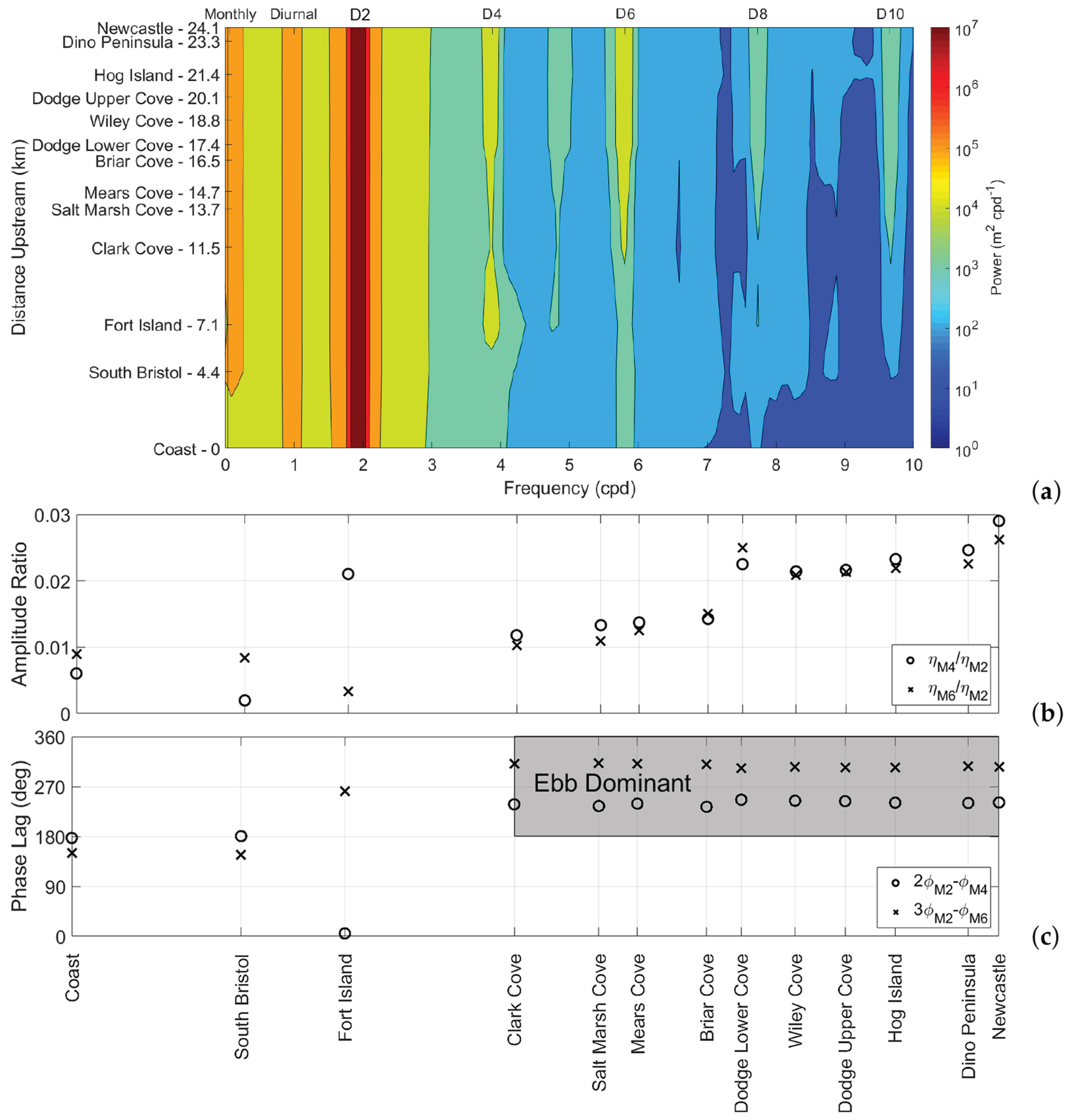
The PSD contour plot of tidal elevation at the 13 sites throughout the sampling period is shown in Figure 2. As expected, the semidiurnal tidal constituent was the most prominent throughout the estuary (S ), followed by the diurnal components (S ). The D4 overtide originated in the shallow region surrounding Fort Island, attenuated through the middle reach and amplified as it propagated landward (S ). The D6 overtide originated north of the bend at Clark Cove, amplifying at the same rate as D4 as it propagated landward (S ). In order to understand the relative significance of overtide amplitudes and phases, it is useful to consider them in terms of the D2 tide. The amplitudes of the D4 and D6 overtides, relative to D2, and their phase lags, defined as and , respectively, are shown in Figure 2.
With this in mind, connections can be drawn from the tidal dynamics of the estuary to tidal variations in water quality. The tidal analysis revealed stronger ebb currents compared to flood, which were induced primarily by bottom friction and depth variational friction induced by the converging estuary. The role of these tidal asymmetries, in conjunction with along-estuary variation in water quality parameters, is explored in the subsequent section.
3.2. Estuarine Dynamics
3.2.1. Coast Analysis
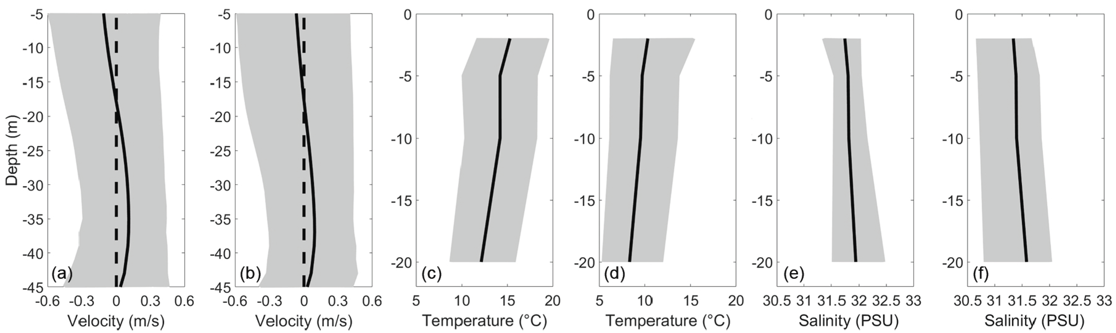
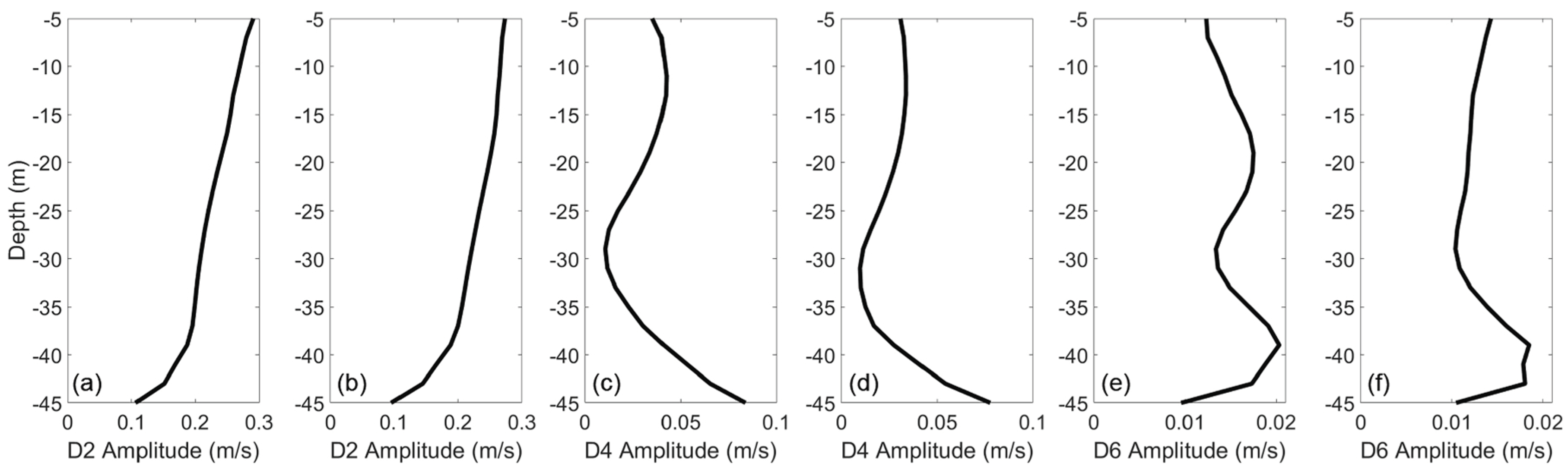
The Damariscotta estuary can be characterized by varying structures in tidal amplitude and subtidal velocity. The estuary originated with a vertically sheared structure near the coast, transitioned to a laterally sheared structure past Briar Cove, and finally to a sort of mixed structure further north. The vertical structure of flow where the estuary meets the Gulf of Maine was a two layer system (Figure 3). During the dry season, from the surface to a depth of 19 m, warmer, lower salinity water flowed out of the estuary, at a maximum velocity of ∼0.05 m/s at the surface. Below 19 m, cooler, higher salinity water flowed into the estuary, with a maximum subtidal velocity of ∼0.07 m/s at a depth of 39 m. Semidiurnal amplitudes were highest at the surface, at ∼0.25 m/s, decreasing gradually to ∼0.20 m/s at 39 m depth, then decreasing steadily to ∼0.07 m/s near the bottom. Quarter-diurnal amplitudes were roughly equal to of semidiurnal amplitudes from the surface down to a depth of 35 m, below which they increase rapidly to equal the semidiurnal amplitudes. Dynamics during the wet season were qualitatively similar to those of the dry season, but tidal amplitudes were about higher, as shown in Figure 4.
The mean temperature at the coast was ∼14 C during the dry season and ∼8 C during the wet season, when ice melt lowers the temperature of the estuary (Table 2). Semidiurnal amplitudes range from to C at the surface, increasing to a maximum at 20 m depth. Throughout the water column, diurnal amplitudes of temperature were about half of the semidiurnal, and the monthly constituent was on the same order of magnitude as the semidiurnal constituent.
The estuary had slightly higher salinity in the dry season than wet, with a mean of PSU compared to PSU. Salinity increased by about PSU, and temperature decreased by about 1 C with depth (Figure 3c–e). Salinity was semidiurnal dominant, with an amplitude of about PSU at the surface and increasing to PSU at 20 m (not shown). The fortnightly and monthly tidal constituents were of larger amplitudes than semidiurnal, at about and PSU, respectively, throughout the water column.
The quarter-diurnal components of temperature and salinity were each about half the amplitude of their respective semidiurnal components, with a qualitatively similar structure throughout the water column. These relatively high quarter-diurnal components were likely a result of the flood/ebb asymmetry inherent in the vertical flow structure. Salinity was higher in the ebb phase at the surface, but higher in the flood phase below 5 m depth (Figure 5). Temperature was the opposite, with higher temperatures during the flood phase at the surface and a higher temperature during the ebb phase below 5 m. Although the turbidity sensor was nonfunctional, the data collected further north at Clark Cove indicate that turbidity was likely enhanced during the ebb phase.
3.2.2. Clark Cove Analysis
Further north, the harmonic analysis of the Clark Cove buoy data indicates that the semidiurnal component of along-channel current velocity near the surface was consistent with the coast, and the fortnightly constituent was enhanced, but the diurnal and quarter-diurnal constituents were diminished. However, the fortnightly, D2, and D4 amplitudes of turbidity were roughly equal in magnitude, at about NTU (Table 2).
Unlike at the coast, salinity at Clark Cove was semidiurnal dominant, with an amplitude of PSU. The monthly and fortnightly amplitudes were lower than the semidiurnal amplitude, at and PSU, respectively, and the quarter-diurnal amplitude was diminished at PSU. Water temperature was also semidiurnal dominant, at C, and interestingly, this harmonic plays a larger role in temperature variation than the day/night cycle, which had an amplitude of C. Monthly and fortnightly amplitudes were and C, respectively, and quarter-diurnal amplitudes were on a similar order of magnitude at C.
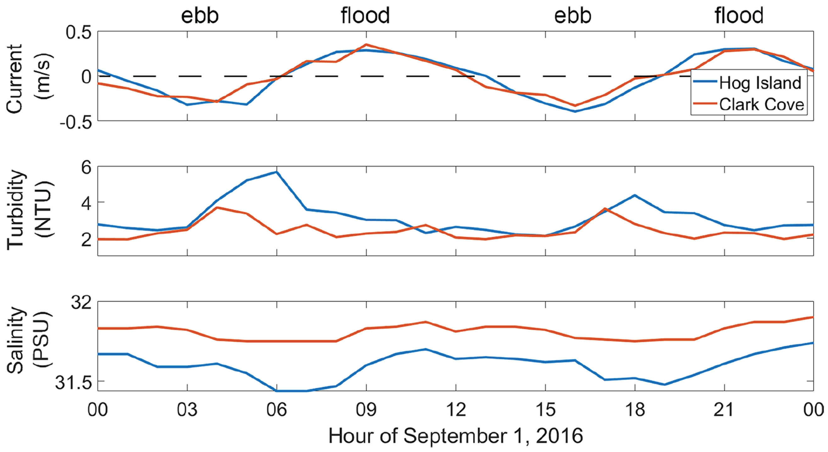
Around Clark Cove, flood-ebb asymmetry began to develop in salinity as well as turbidity. An example of this is shown in Figure 5. Turbidity at the surface was higher during ebb than flood, and salinity was higher during the slack period after flood than after ebb. This asymmetry became even more noticeable further north, near Hog Island. Chlorophyll measurements tend to be flood–ebb symmetric, and the primary tidal constituents were the solar harmonics, such as K1, S2, and S4. The S4 amplitude (∼0.044 g/L) was a fraction of the S2 amplitude (∼0.22 g/L), but the tridiurnal (SK3) harmonic was significant at an amplitude of ∼0.13 g/L.
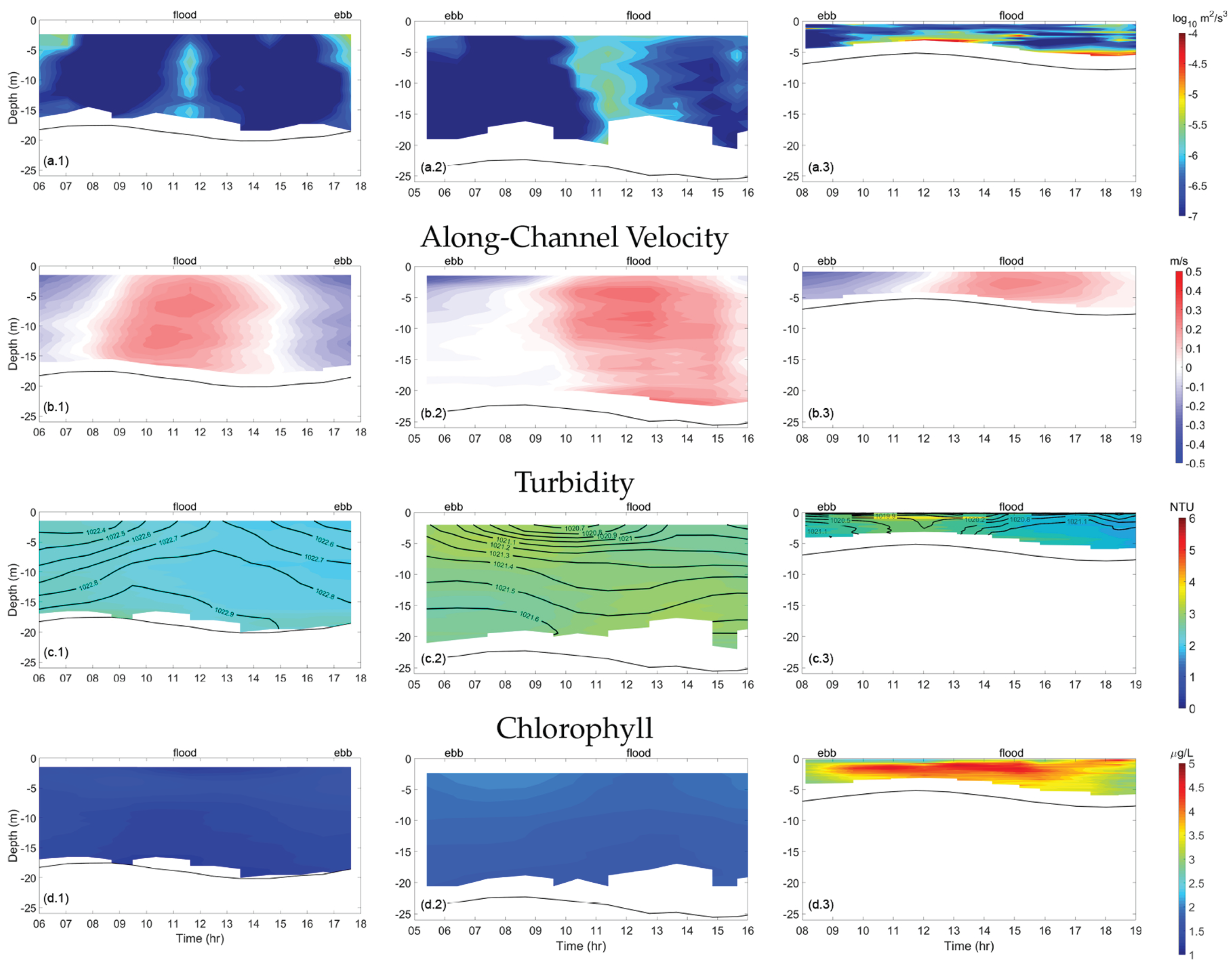
Figure 6 and Figure 7 show transect measurements for TKE dissipation, along-channel velocity, turbidity, and chlorophyll at Clark Cove, Glidden Ledges, and Hog Island. Density is also shown to illustrate the relationship between increased stratification and an uneven spatial distribution of turbidity.
In neap tide, semidiurnal tidal amplitudes of current velocity were highest at the surface, at m/s, and decreased to m/s near the bottom (Figure 4). Quarter-diurnal amplitudes were highest at the bottom, as m/s or 40% of semidiurnal. Flow patterns in spring tide were qualitatively similar, with a maximum semidiurnal amplitude of m/s at the surface and a minimum amplitude of m/s at the bottom. Quarter-diurnal amplitudes were highest at the bottom, with an amplitude of m/s, also about 40% of semidiurnal.
During neap tide, was also elevated during the ebb phase and highest at the surface (∼), extending downwards but not reaching the bottom (Figure 6a.1). TKE dissipation was relatively negligible (∼) during high tide and low tide and was similarly weak during the flood phase, when landward along-channel velocity was highest. These asymmetric patterns result in having a primarily semidiurnal pattern at the surface and quarter-diurnal patterns at the bottom.
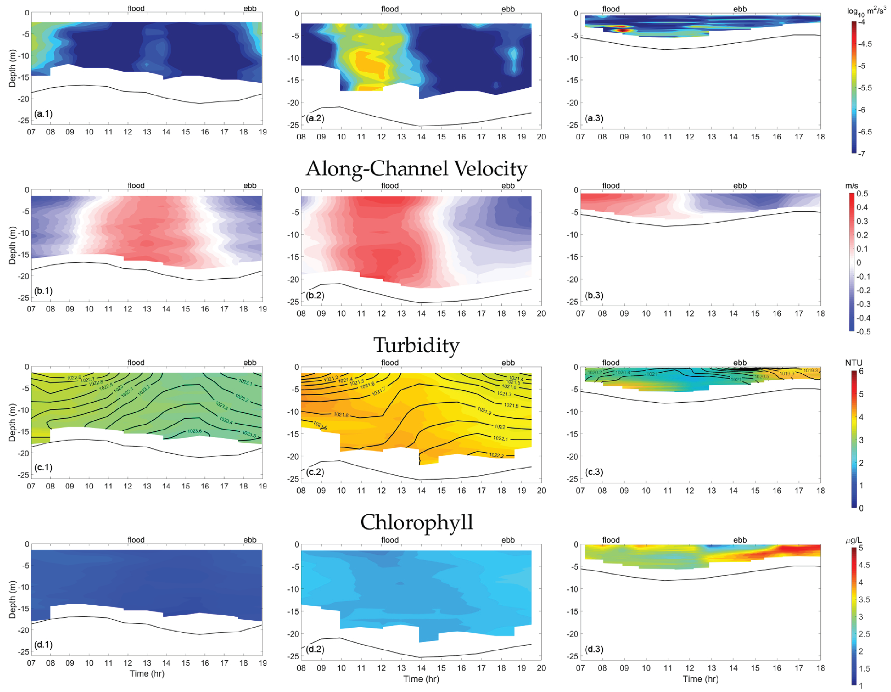
TKE dissipation () measured in the channel of Clark Cove was largest in between the ebb and flood phases (Figure 7a.1). During spring tide, was strongest at the end of flood phase, when velocities reach a maximum of 0.8 m/s, throughout the water column but especially at the surface (∼). TKE dissipation was elevated during the end of the ebb phase as well, when seaward along-channel velocity diminishes, but to a lesser extent (∼) at about 5 m below the surface. Since was largest at the surface during ebb and greatest below the surface during the flood, this indicates that dissipation during flood was linked to bottom friction, but dissipation during ebb was not. This has implications for tidal patterns in turbidity (Figure 7c).
Turbidity tended to be higher during spring tide (∼3.4 NTU) than neap tide (∼2.4 NTU) and tended to be elevated throughout the water column during the late ebb phase, when the water level was shallowest. According to buoy data, chlorophyll concentration, as opposed to turbidity, was slightly higher during neap tide (∼2.0 g/L) than spring tide (∼1.9 g/L) and was elevated at the surface during each slack period. In other words, turbidity tended to be correlated with elevated , and chlorophyll tended to be correlated with diminished .
3.2.3. Glidden Ledges Analysis
The next transect was situated immediately north of Glidden Ledges, near Dodge Lower Cove. TKE dissipation was highest during the flood phase, throughout the water column (∼) as high velocity water was forced through the constriction (Figure 6a.2). TKE dissipation was elevated only at the surface during the slack period after flood and at the end of the ebb phase (∼). These patterns were larger during spring tide, with a maximum of (∼) near the middle of the water column, and during the ebb phase, was somewhat elevated away from the bottom boundary (∼) (Figure 7a.2). This contributed to a higher quarter-diurnal amplitude during spring tide.
In neap tide, in the channel region, turbidity was highest during the ebb phase near the surface and during the flood phase near the bottom, with a maximum of ∼ NTU (Figure 6c.2). During spring tide, turbidity was higher during the flood phase than during ebb, at a maximum of ∼ NTU, and significantly higher in spring tide (mean of ∼ NTU) than neap tide (mean of ∼ NTU). High turbidity was linked to high only when the region of high extended all the way to the bottom. Throughout the cross-section, chlorophyll concentration was elevated at the beginning and end of ebb, at the surface, with a maximum of ∼ g/L in neap and spring tide. This increased chlorophyll concentration was likely originating upstream, near Hog Island.
3.2.4. Hog Island Analysis
Finally, attention is focused on the transects conducted in the northern reach of the estuary near Hog Island, where much of the aquaculture activity is located. TKE dissipation was highest during early flood (∼), and during peak flood, was much larger at the bottom of the channel compared to the rest of the water column (Figure 6a.3). The northern reach had both higher turbidity and higher chlorophyll levels than the rest of the estuary. Also, the flood–ebb asymmetry in turbidity and salinity that began near Clark Cove was most extreme in the northern reach (Figure 5). During peak ebb, turbidity reaches a maximum of 8 NTU, and chlorophyll reaches a maximum of ∼5 g/L, the highest observed at any point along the estuary. It was also the only region along the estuary at which high turbidity and chlorophyll were correlated. During flood phase, chlorophyll was elevated near the surface, and turbidity was elevated near the bottom, as increased stratification inhibits productivity below the surface.
During peak ebb, was elevated throughout the water column (∼). TKE dissipation was actually higher in peak flood during neap tide than during spring tide (Figure 6a.3). In neap tide, turbidity was largest (∼ NTU) throughout the water column from end of ebb to beginning of flood (Figure 6c.3). This was due to the absence of a salinity intrusion front during this period.
During spring tide, turbidity was largest (∼ NTU) in the lower water column during the end of flood, due to a salinity intrusion front introducing stratification that limited the upward extent of turbidity. During the ebb phase, elevated turbidity encompasses the entire water column, not just because of the shallow water depth but also because the salinity intrusion front was advected seaward, allowing for turbidity to reach the surface.
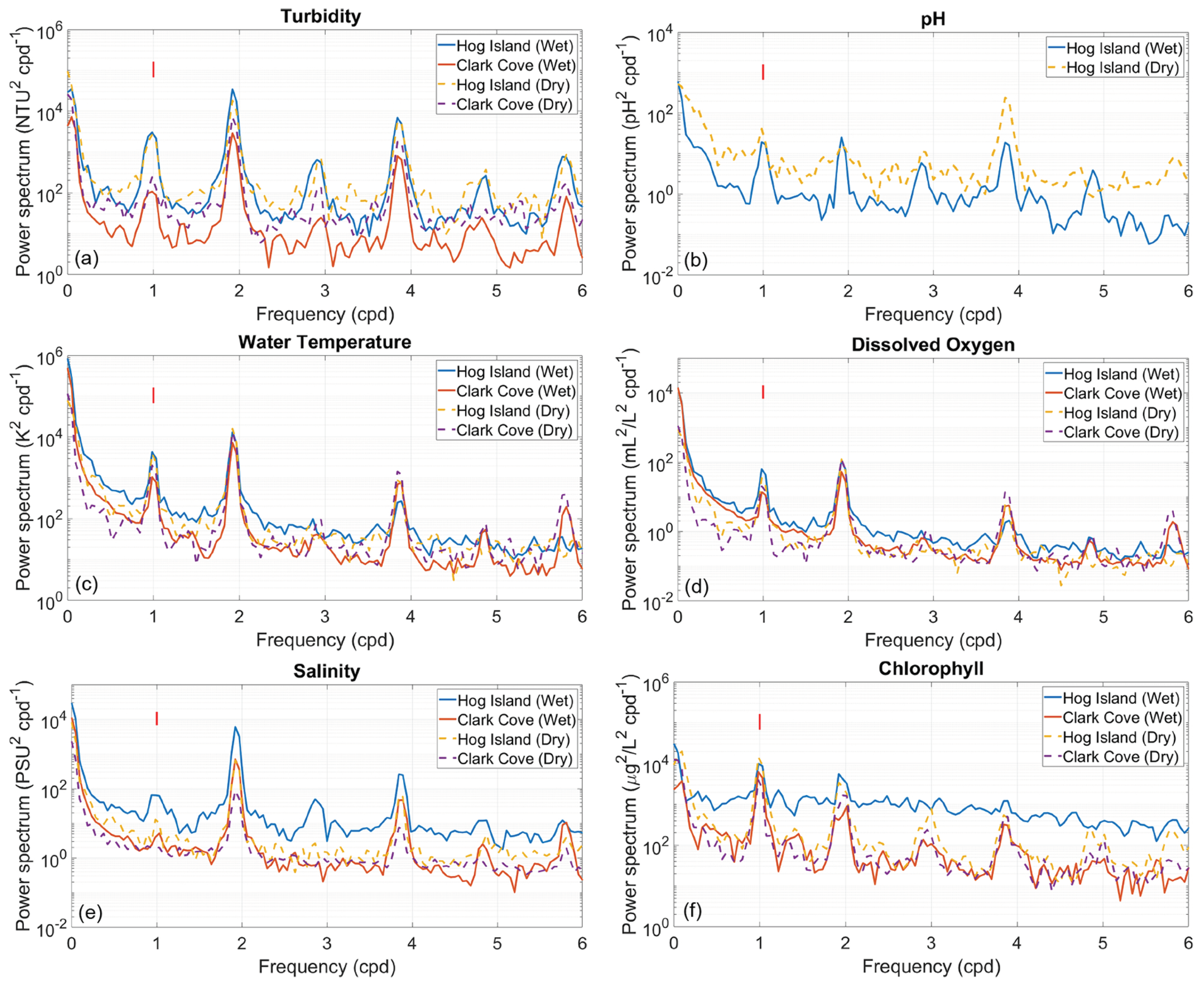
According to the LOBO buoy located near Hog Island, during the dry season, turbidity was higher during ebb than flood, and chlorophyll was roughly flood–ebb symmetric. D4 amplitudes of turbidity were about half the D2 amplitude (∼ NTU compared to ∼ NTU), and D2, D3, and D4 amplitudes of chlorophyll were roughly equal (∼ g/L). The D3 amplitude arises due to nonlinear interactions between the diurnal and semidiurnal harmonics. During the wet season, turbidity was still higher during the ebb phase, but chlorophyll was higher during the flood phase. Tidal amplitudes of turbidity and chlorophyll were reduced by about due to increased stratification in the salinity intrusion front and colder temperatures, respectively. Turbidity tended to be much higher in spring tide than neap (∼8 NTU compared to ∼3 NTU), whereas chlorophyll tended to be higher in neap (∼6 g/L compared to ∼2 g/L). The transect measurements show that this discrepancy between turbidity and chlorophyll was likely due to increased TKE dissipation correlating with increased turbidity but decreased chlorophyll (Figure 8).
A particularly unusual phenomenon during the dry season was that in terms of acidity, D4 amplitudes of pH were actually twice those of D2 (∼ compared to ∼0.026), as shown in Figure 8b. However, no clear pattern of flood–ebb symmetry was apparent, as the pH value tended to vary more seasonally than tidally. Dissolved oxygen tended to be flood–ebb symmetric, according to the buoy measurements, and the D4 harmonic amplitudes were not particularly large (Figure 8d).
3.3. Tidal Influence on Water Quality
Power spectral density plots for chlorophyll a, dissolved oxygen, pH, salinity, water temperature, and turbidity, divided between wet and dry season, are shown in Figure 8. As a point of reference, the spectral power density of the tides at both locations was about at D2 and at D4 and D6, for a power ratio of about . The spectral density was about at the diurnal frequency. This means that if the power of a certain metric at D4 was at least times the power at D2 (or at diurnal at least times the power), then the corresponding harmonic has a disproportionately strong effect on that metric.
4. Discussion
This paper illustrates how irregularities in estuarine channel geometry, such as curvature and constrictions, contribute to tidal nonlinearity in water quality in the middle and upper reaches of a tidally driven estuary. Specifically, channel complexities contribute to intratidal harmonics of water elevation and current velocity, which in turn result in flood–ebb asymmetries. These asymmetries likely enhance net surface transport of suspended particulates, which are connected to all metrics of water quality relevant to shellfish aquaculture.
4.1. Upstream Tidal Evolution
Landward from the coast to the city of Newcastle, the diurnal constituent of water elevation declined slightly, and the semidiurnal constituent amplified slightly. On the other hand, the overtide harmonics, although small relative to the semidiurnal harmonic, were amplified by two- or threefold up the estuary. The exception was at Fort Island where the D4 overtide amplitude increased to 2.2% of D2, then dropped down to 1% of D2 at Clark Cove. The D2 tide was standing, although it did exhibit progressive characteristics typical in short converging estuaries, as the tidal propagation velocity was proportional to the e-folding length [37]. The tide advanced by throughout the estuary, with the fastest increase in phase through the Fort Island constriction. In an idealized prismatic channel, one might expect water level amplitudes and current velocity amplitudes to be directly correlated, and for most harmonics, this was somewhat the case. The one exception was the quarter-diurnal harmonic, of which the current velocity but not the water level amplitude was diminished near Clark Cove. In general, overtides are amplified where the river is narrowest [38]. The high amplification of D4 between South Bristol and Fort Island can be explained by the constrictions around the island, which may enhance overtides via wave reflection [39] and bed stress [40].
The D4 overtide attenuated in the region between Clark Cove and Briar Cove and amplified as it was forced through the Glidden Ledges constriction near Briar Cove, reaching a maximum amplitude of 2.9% of D2 at New Castle. Since the D4 overtides are caused by a variety of forces, including bottom friction, depth variational friction, and, to a lesser extent, advection and nonlinear continuity [41], the influence of constrictions on this constituent are varied and often unintuitive [6]. On the other hand, the D6 overtide amplitude, as it was solely caused by bottom friction, was inversely proportional to the estuary depth. Similarly to D4, there was a strong amplification of D6 through Briar Cove, and it reaches a maximum relative amplitude of 2.3% of D2 at Newcastle. This implies that the overtide amplitudes were amplified by the shape of the converging or constricted channels.
The relative phase lag between the D2, D4, and D6 tides can be used to determine flood/ebb dominance along the estuary, meaning that either flood or ebb flow is of a higher velocity than the other, although the dominant phase is of shorter duration. North of Clark Cove, the phase lag between D2 and D4 was about , which suggests ebb dominance by the definition proposed by Friedrichs and Aubrey [42]. By averaging over flood and ebb cycles, the flood phase tended to be of longer duration than the ebb phase, up to 25 min longer near Newcastle, but the ebb currents were on average about 12% stronger. This means that over sufficiently long periods of time, any particulates in the estuary will be flushed out through the river mouth. The mean amplitude of flood currents near Hog Island, according to the LOBO buoy, was 0.233 m/s, compared to ebb currents with a mean amplitude of 0.261 m/s. Similarly, at Clark Cove, the mean amplitude of flood currents was 0.119 m/s, whereas ebb currents had a mean amplitude of 0.129 m/s. The phase lag between D2 and D6 north of Clark Cove was about 300, and according to Blanton et al. [43], the D6 overtide had a distortion effect on the tidal cycle, contributing further to ebb tidal dominance based on the phase angle .
4.2. Dissipation and Water Quality
Throughout the estuary, TKE dissipation () tended to be elevated during peak flood and peak ebb. This implies that manifests as a quarter-diurnal harmonic, as it oscillates twice during a semidiurnal tidal cycle. However, also tended to be larger either in the flood or in the ebb phase, which implies that intratidal asymmetry presents itself as a semidiurnal harmonic. As turbidity is linked to at the surface, the harmonics in serve as an explanation for why the D4 and D2 harmonics of turbidity were on the same order of magnitude, even though D4 amplitudes in tidal elevation and surface velocity were a fraction of the D2 amplitudes. Chlorophyll concentration had similar harmonics but oscillates out of phase with turbidity. Specifically, chlorophyll tended to be elevated during the slack periods when turbidity was lowest. Chlorophyll also tended to be flood–ebb symmetric, except in the northern reach during the wet season.
The estuary had a vertically sheared structure at the coast, as higher salinity water from the Gulf of Maine flows inland below the surface and fresh water flows seaward at the surface. The vertical structure persisted at the Clark Cove bend and was most apparent during peak ebb and flood. During neap tide, was elevated at the surface during the slack period between flood and ebb and throughout the water column during the slack period between ebb and flood.
Elevated levels of correlated with similarly elevated levels of turbidity only if the region of high extended to the bottom, where turbulence and shear stresses could enhance the suspension of sediment. Increased stratification during flood phase limits the extent of upward extent of sediment suspension, contributing to reduced turbidity at the surface [44]. Therefore, elevated turbidity in the slack period between flood and ebb was observed at Clark Cove only in spring tide, when was increased throughout the entire water column. Chlorophyll concentrations were by and large negligible near Clark Cove, although, as expected, they were somewhat higher at the surface than at the bottom.
Further upstream, at the Glidden Ledges constriction, the flow dynamics were heavily influenced by the 600 m constriction, in which flow was forced through the constriction and into the eastern channel during flood phase [6]. In this region, elevated was observed throughout the water column but only in the flood phase. This time period of high correlated with elevated turbidity as sediment was suspended, and with reduced chlorophyll concentration as sunlight was blocked. During the ebb phase, current velocities were extremely diminished below the surface. This encourages the continued suspension of sediment, which was why turbidity was observed at the surface in this phase.
In the northern reach, near Hog Island, the structure becomes a mix of lateral and vertical shear as the distorting effects of Glidden Ledges were somewhat diminished. Here, both turbidity and chlorophyll levels were significantly higher than any other region of the estuary, and this was the case throughout the water column and in both the flood and ebb phases. The higher turbidity levels were likely due to the high volume of sediment storage, as well as the shallow bathymetry that allowed surface-level shear patterns to extend to the estuarine bottom. Chlorophyll was elevated because the temperature here was on average 2 C higher than the middle and outer estuary, which makes the region especially viable for aquaculture. TKE dissipation was highest at the bottom throughout the entire tidal cycle, and throughout the water column during the flood phase.
At both Clark Cove and Hog Island, the D4 constituent of turbidity was on the same magnitude of spectral power as the D2 constituent, at least at the surface (Figure 8a). This is because turbidity tended to elevate during both the flood and ebb phase, resulting in four oscillations per day. During the dry season, this D4 harmonic in turbidity was observed throughout the water column, while during the wet season, it was primarily observed below the surface (not shown). The monthly tidal constituents were roughly equal in magnitude to the D2 and D4 constituents, which is common in tidally-driven estuaries [12]. Chlorophyll concentration oscillates primarily on a solar diurnal basis, as sunlight is necessary for plankton productivity. Higher frequency oscillations do occur in chlorophyll, but these were not due to the tides. They were due to intratidal interactions of the daily cycle of light exposure with vertical stratification in chlorophyll concentration [45].
4.3. Harmonics of Water Quality
Speaking more generally, intratidal asymmetry in along-channel current velocity tended to have an outsized influence in intratidal asymmetry on water quality metrics related to particulate concentration, especially due to their links to TKE dissipation. This was especially true for turbidity, which we used as a proxy for suspended sediment, and for chlorophyll concentration. Elevated turbidity, as measured by the surface buoys near Clark Cove and Hog Island, was heavily correlated with near the surface. Just as Glidden Ledges divided the estuary between a vertical and lateral shear structure, it also divided the estuary as to whether at the surface was higher during the ebb or flood phase. South of Glidden Ledges, the estuary behaved mainly as a converging channel, in which high salinity water flowed through the bottom layer of the estuary during flood phase, rose to the surface during the slack period, and was transported out during ebb. North of Glidden Ledges, surface was higher during flood as water was forced through the constriction and into the channel. Salinity was higher during spring tide than neap tide, as salt water was able to travel a further distance inward from the Gulf of Maine. However, and turbidity were higher in flood phase during neap tide because the lower velocity waters allow for greater suspension of sediment. Because of the high quantity of stored sediment and reflection off the Damariscotta Lake Dam, monthly and semidiurnal amplitudes of turbidity were higher in the wet season than the dry season in the northern reach.
The tidal composition of salinity was comparable to that of the along-channel current velocity. Salinity tended to be elevated when strong flood velocities transport saltier water landward from the Gulf Maine. Water temperature was highest during ebb, as shallower, upstream water that had been warmed by the sun was being advected seaward past the LOBO buoy and had a diurnal amplitude of about 4 C. Dissolved oxygen, on the other hand, tended to oscillate alongside with flood tide, as the surface tended to be more oxygen-rich. For both of these metrics, the relative power of the D4 and D6 components was the same as that of the D2 constituent. Finally, pH was unusual in that the D4 component was significantly more influential than the D2 component, likely due to intratidal interactions between tidal cycles of turbidity and the lower pH of sediment porewater. Since along-channel flow harmonics were correlated with TKE dissipation harmonics at double the frequency [14], explaining tidal relationships between TKE dissipation and water quality metrics helps to explain the relatively strong intratidal components of turbidity, pH, water temperature, and dissolved oxygen.
The harmonics of pH near Hog Island were especially unusual in that the D4 component was the primary driver of variability, especially in the dry season; however, no clear pattern of flood–ebb asymmetry was apparent. One possible explanation is that peak flood and ebb velocities interacting with the bottom driven by D4 overtides mobilize sediment into the water column. On a quarter-diurnal time scale, turbidity, the best indicator of suspended sediment, was in phase with along-channel currents, and the water was most turbid when currents were highest. Sediment porewater had lower pH and oxygen than regular river water [18], and sediment blocks sunlight, which affects temperature and chlorophyll levels.
The research presented in this paper demonstrates that frictional forces imposed by an irregular bathymetry influence tidal harmonics with a disproportionately significant effect on the analogous harmonics of turbidity, salinity, and pH. As the depth variation and bottom friction nonlinear forcing mechanisms were affected by flow rates and estuarine depth, their affects may be amplified or diminished by rising sea levels and higher precipitation. The northern region is exceptionally viable for oyster aquaculture because its lateral shear patterns assist in the retention of suspended nutrient particles. A possible consequence of climate change is that reduced friction may decrease exchange rates and transport distances. The upper estuary may witness higher turbidity and oxygen levels, and lower salinity and acidity, due to increased flushing times. However, should Glidden Ledges become overflooded by frequent storm events, materials may flush out of the estuary more rapidly. This would be a detriment to oyster aquaculture, and more research is necessary to determine the effects of climate change on particle retention in the northern region.
5. Conclusions
The irregular, converging bathymetry of the Damariscotta River Estuary significantly affects its tidal dynamics, including its tidal amplitudes, shear structure, and material transport rates. Each region of the estuary has its own unique nonlinear forcing dynamics that affect rates of dissipation and play disproportionately large roles in the health of the estuary. For example, multiple constrictions throughout the estuary cause along-channel shear flow to evolve from a vertical to a lateral to a diagonal structure, and the overtide components of water elevation steadily amplify upstream. These overtides, along with the shear structure, result in enhanced harmonic patterns of sediment suspension and TKE dissipation. Enhanced TKE dissipation causes enhanced turbidity if the region of high dissipation extends to the bottom, and tidal cycles in turbidity can be linked to opposing tidal cycles in chlorophyll concentration. Most importantly, the lateral shear structure in the upper estuary also assists in particle retention, which aids the region in being a particularly suitable site for shellfish aquaculture.
The dynamics of the estuary and its effects on water quality metrics are important to understanding both the key sites for aquaculture and the effects of climate change on aquaculture, and with additional flow data, we can shed more light on the behavior of fluid and material transport in other glacially carved estuaries. Numerical models that attempt to predict ideal sites for establishing aquaculture farms would be advised to consider patterns of irregular bathymetry in their framework.
Author Contributions
Conceptualization, B.L., K.H., and L.R.; Data curation, B.L.; Formal analysis, B.L.; Investigation, B.L. and Z.L.; Project administration, K.H.; Resources, K.H.; Validation, B.L.; Visualization, B.L. and K.H.; Writing—original draft, B.L.; Writing—review and editing, L.R.
Funding
This research was funded by the Sustainable Ecological Aquaculture Network (NSF #1355457) and a University of Maine Rising Tide SEED Grant.
Acknowledgments
Thank you to Kyah Lucky, Elliot Huguenard, and Emma Murowinski for their assistance with field data collection.
Conflicts of Interest
The authors declare no conflict of interest. The funders had no role in the design of the study; in the collection, analyses, or interpretation of data; in the writing of the manuscript, or in the decision to publish the results.
References
- Nguyen, N.; Yori, W. Technology Assessment in Aquaculture of Dominant and Potential Species in Maine; Technical Report; University of Maine: Orono, ME, USA, 2015. [Google Scholar]
- Nelson, M. Maine Aquaculture Harvest Data; Technical Report; Department of Marine Resources: Augusta, Maine, 2016.
- Sanger, D.; Sanger, M.J. The Damariscotta Oyster Shell Heaps. Northeast. Nat. 1997, 4, 93–102. [Google Scholar] [CrossRef]
- Pershing, A.J.; Alexander, M.A.; Hernandez, C.M.; Kerr, L.A.; Bris, A.L.; Mills, K.E.; Nye, J.A.; Record, N.R.; Scannell, H.A.; Scott, J.D.; et al. Slow adaptation in the face of rapid warming leads to collapse of the Gulf of Maine cod fishery. Science 2015, 350, 809–812. [Google Scholar] [CrossRef] [PubMed] [Green Version]
- Reguero, B.G.; Losada, I.J.; Méndez, F.J. A recent increase in global wave power as a consequence of oceanic warming. Nat. Commun. 2019, 10. [Google Scholar] [CrossRef] [PubMed] [Green Version]
- Lieberthal, B.; Huguenard, K.; Ross, L.; Bears, K. The Generation of Overtides in Flow Around a Headland in a Low Inflow Estuary. J. Geophys. Res. Ocean. 2019. [Google Scholar] [CrossRef]
- Liu, Z.; Huguenard, K. Hydrodynamic response of a floating aquaculture farm in a partially stratified estuary. J. Geophys. Res. Ocean. 2019, submitted. [Google Scholar]
- Parker, B. Friction Effects on the Tidal Dynamics of a Shallow Estuary. Ph.D. Thesis, Johns Hopkins University, Baltimore, MD, USA, 1984. [Google Scholar]
- Moskalski, S.M.; Sommerfield, C.K.; Wong, K.C. Oceanic and Hydrologic Influences on Flow and Water Properties in the St. Jones River Estuary, Delaware. Estuaries Coasts 2011, 34, 800–813. [Google Scholar] [CrossRef]
- Zarzuelo, C.; López-Ruiz, A.; Díez-Minguito, M.; Ortega-Sánchez, M. Tidal and subtidal hydrodynamics and energetics in a constricted estuary. Estuar. Coast. Shelf Sci. 2017, 185, 55–68. [Google Scholar] [CrossRef]
- Gräwe, U.; Burchard, H.; Müller, M.; Schuttelaars, H.M. Seasonal variability in M2 and M4 tidal constituents and its implications for the coastal residual sediment transport. Geophys. Res. Lett. 2014, 41, 5563–5570. [Google Scholar] [CrossRef] [Green Version]
- Díez-Minguito, M.; Baquerizo, A.; De Swart, H.E.; Losada, M.A. Structure of the turbidity field in the Guadalquivir estuary: Analysis of observations and a box model approach. J. Geophys. Res. Ocean. 2014, 119, 7090–7204. [Google Scholar] [CrossRef] [Green Version]
- Souza, A.J.; Alvarez, L.G.; Dickey, T.D. Tidally induced turbulence and suspended sediment. Geophys. Res. Lett. 2004, 31. [Google Scholar] [CrossRef] [Green Version]
- Simpson, J.H.; Rippeth, T.P.; Campbell, A.R. The phase lag of turbulent dissipation in tidal flow. In Interactions Between Estuaries, Coastal Seas and Shelf Seas; Yanagi, T., Ed.; Terrapub: Tokyo, Japan, 2000; pp. 57–67. [Google Scholar]
- Schoellhamer, D.H. Influence of salinity, bottom topography, and tides on locations of estuarine turbidity maxima in northern San Francisco Bay. Proc. Mar. Sci. 2000, 3, 343–357. [Google Scholar] [CrossRef]
- Sommerfield, C.K.; Wong, K.C. Mechanisms of sediment flux and turbidity maintenance in the Delaware Estuary. J. Geophys. Res. Ocean. 2011, 116, 1–16. [Google Scholar] [CrossRef]
- Rippeth, T.P.; Simpson, J.H.; Williams, E.; Inall, M.E. Measurement of the Rates of Production and Dissipation of Turbulent Kinetic Energy in an Energetic Tidal Flow: Red Wharf Bay Revisited. J. Phys. Oceanogr. 2003, 33, 1889–1901. [Google Scholar] [CrossRef] [Green Version]
- Hales, B.; Emerson, S.; Archer, D. Respiration and dissolution in the sediments of the western North Atlantic: Estimates from models of in situ microelectrode measurements of porewater oxygen and pH. Deep-Sea Res. Part I 1994, 41, 695–719. [Google Scholar] [CrossRef]
- Kesaulya, I.; Leterme, S.C.; Mitchell, J.G.; Seuront, L. The impact of turbulence and phytoplankton dynamics on foam formation, seawater viscosity and chlorophyll concentration in the eastern English Channel Turbulence Foam Plankton rheology Phytoplankton. Oceanologia 2008, 50, 167–182. [Google Scholar]
- Liu, B.; de Swart, H.E. Impact of river discharge on phytoplankton bloom dynamics in eutrophic estuaries: A model study. J. Mar. Syst. 2015, 152, 64–74. [Google Scholar] [CrossRef]
- Uncles, R.J. Estuarine physical processes research: Some recent studies and progress. Estuar. Coast. Shelf Sci. 2002, 55, 829–856. [Google Scholar] [CrossRef] [Green Version]
- Baines, S.B.; Fisher, N.S.; Doblin, M.A.; Cutter, G.A.; Cutter, L.S.; Cole, B. Light dependence of selenium uptake by phytoplankton and implications for predicting selenium incorporation into food webs. Limnol. Oceanogr. 2004, 49, 566–578. [Google Scholar] [CrossRef] [Green Version]
- Paerl, H.W.; Valdes, L.M.; Peierls, B.L.; Adolf, J.E.; Harding, L.J.W. Anthropogenic and climatic influences on the eutrophication of large estuarine ecosystems. Limnol. Oceanogr. 2006, 51, 448–462. [Google Scholar] [CrossRef] [Green Version]
- Silvert, W. Assessing environmental impacts of finfish aquaculture in marine waters. Aquaculture 1992, 107, 67–79. [Google Scholar] [CrossRef]
- Smith, C.S.; Ito, M.; Namba, M.; Nakaoka, M. Oyster aquaculture impacts Zostera marina epibiont community composition in Akkeshi-ko estuary, Japan. PLoS ONE 2018, 13, e0197753. [Google Scholar] [CrossRef] [PubMed]
- Dumbauld, B.R.; Ruesink, J.L.; Rumrill, S.S. The ecological role of bivalve shellfish aquaculture in the estuarine environment: A review with application to oyster and clam culture in West Coast (USA) estuaries. Aquaculture 2009, 290, 196–223. [Google Scholar] [CrossRef]
- Hanson, D. Thunderhead Technologies. 2017. Available online: http://www.thunderheadtech.com/NewHarbor1se/ (accessed on 1 October 2019).
- Chandler, E.A. Sediment Accumulations Patterns in the Damariscotta River Estuary. Ph.D. Thesis, University of Maine, Orono, ME, USA, 2016. [Google Scholar]
- Shipp, C.R.; Belknap, D.F.; Kelley, J.T. Seismic-Stratigraphic and Geomorphic Evidence for a Post- Glacial Sea-Level Lowstand in the Northern Gulf of Maine. J. Coast. Res. 1991, 7, 341–364. [Google Scholar] [CrossRef]
- McAlice, B.J.; Grant, M.S. A Preliminary Oceanographic Survey of the Damariscotta River Estuary, Lincoln County, Maine; Maine Sea Grant Technical Report; University of Southern Maine: Portland, ME, USA, 1977; Available online: http://digitalcommons.usm.maine.edu/cgi/viewcontent.cgi?article=1105&context=me_collection (accessed on 7 December 2019).
- Snyder, J.; Boss, E.; Weatherbee, R.; Thomas, A.C.; Brady, D.; Newell, C. Oyster Aquaculture Site Selection Using Landsat 8-Derived Sea Surface Temperature, Turbidity, and Chlorophyll a. Front. Mar. Sci. 2017, 4, 190. [Google Scholar] [CrossRef] [Green Version]
- Martin, T.C. Light Dynamics in the Damariscotta River Estuary with Implications for Microphytobenthos. Ph.D. Thesis, University of Maine, Orono, ME, USA, 2017. [Google Scholar]
- Van Beers, W.; Kleijnen, J. Kriging Interpolation in Simulation: A Survey. In Proceedings of the 2004 Winter Simulation Conference, Washington, DC, USA, 5–8 December 2004; Volume 1, pp. 107–115. [Google Scholar] [CrossRef]
- Pawlowicz, R.; Beardsley, B.; Lentz, S. Classical tidal harmonic analysis including werror estimates in MATLAB using T_TIDE. Comput. Geosci. 2002, 28, 929–937. [Google Scholar] [CrossRef]
- Jay, D.A.; Kukulka, T. Revising the paradigm of tidal analysis—The uses of non-stationary data. Ocean Dyn. 2003, 53, 110–125. [Google Scholar] [CrossRef]
- Thomson, R.E.; Emery, W.J. Data Analysis Methods in Physical Oceanography; Newnes: London, UK, 2014. [Google Scholar] [CrossRef]
- Friedrichs, C.T.; Aubrey, D.G. Tidal propagation in strongly convergent channels. J. Geophys. Res. 1994, 99, 3321–3336. [Google Scholar] [CrossRef]
- Gallo, M.N.; Vinzon, S.B. Generation of overtides and compound tides in Amazon estuary. Ocean Dyn. 2005, 55, 441–448. [Google Scholar] [CrossRef]
- Díez-Minguito, M. Tidal Wave Reflection From the Closure Dam in the Guadalquivir Estuary (SW Spain). Coast. Eng. Proc. 2012, 1, 58. [Google Scholar] [CrossRef]
- Giese, B.S.; Jay, D.A. Modelling Tidal Energetics of the Columbia River Estuary. Estuar. Coast. Shelf Sci. 1989, 29, 549–571. [Google Scholar] [CrossRef]
- Wang, Z.B.; Jeuken, C.; Vriend, H.J.D. Tidal Asymmetry and Residual Sediment Transport in Estuaries: A Literature Study and Application to the Western Scheldt; Technical Report; Deltares: Delft, The Netherlands, 1999. [Google Scholar]
- Friedrichs, C.T.; Aubrey, D.G. Non-linear distortion in shallow well-mixed estuaries: A synthesis. Estaurine Coast. Shelf Sci. 1988, 27, 521–545. [Google Scholar] [CrossRef]
- Blanton, J.O.; Lin, G.; Elston, S.A. Tidal current asymmetry in shallow estuaries and tidal creeks. Cont. Shelf Res. 2002, 22, 1731–1743. [Google Scholar] [CrossRef]
- Geyer, W.R. The importance of suppression of turbulence by stratification on the estuarine turbidity maximum. Estuaries 1993, 16, 113–125. [Google Scholar] [CrossRef]
- Doerffer, R.; Fischer, J. Measurement and model simulation of sun stimulated chlorophyll fluorescence within a daily cycle. Adv. Space Res. 1987, 7, 117–120. [Google Scholar] [CrossRef]
Figure 1.
Collection sites along Damariscotta River on the coast of Maine. Water elevation data were collected at thirteen sites from July to November 2016, and current and water quality data were collected at three sites indicated by red dots. The red lines indicate transects that were collected in roughly half-hour intervals over two days in spring and neap tide at Clark Cove in April–May 2017, at Glidden Ledges in April–May 2017, and at Hog Island in June 2017. The contours represent still water level in m.

| Location | Distance (km) | Data Collected | |
| 1 | Coast | 0 | Tides, Currents (vertical profile), |
| Wind, Water Quality | |||
| 2 | South Bristol | 4.4 | Tides |
| 3 | Fort Island | 7.1 | Tides, Transects |
| 4 | Clark Cove | 11.5 | Tides, Currents (surface), |
| Atmospheric Pressure, Water Quality | |||
| 5 | Salt Marsh Cove | 13.7 | Tides |
| 6 | Mears Cove | 14.7 | Tides |
| 7 | Briar Cove | 16.5 | Tides |
| 8 | Dodge Lower Cove | 17.4 | Tides, Transects |
| 9 | Wiley Cove | 18.8 | Tides |
| 10 | Dodge Upper Cove | 20.1 | Tides |
| 11 | Hog Island | 21.4 | Tides, Currents (surface), |
| Water Quality, Transects | |||
| 12 | Dino Peninsula | 23.3 | Tides |
| 13 | Newcastle | 24.1 | Tides |
Figure 2.
(a) Power spectral density contour plot of tidal elevation at each of the sampling sites. The x-axis represents the tidal frequency (in cycles per day)l, the y-axis represents the distance along the river, and Dn represents the nth-diurnal tidal species. (b,c) Relative amplitude and phase lag of D4 and D6 overtides, compared to D2 tides.

Figure 3.
Mean and tidal range of along-channel flow velocity, temperature, and salinity at the coast of the Damariscotta estuary during wet season. (a,c,e) represent dry season, and (b,d,f) represent wet season. Positive velocity represents landward flow, and the shaded areas represent the range of values in a typical tidal cycle.

Figure 4.
D2, D4, and D6 amplitudes of along-channel flow velocity at the coast of the Damariscotta estuary during wet season. (a,c,e) represent dry season, and (b,d,f) represent wet season.
Figure 4.
D2, D4, and D6 amplitudes of along-channel flow velocity at the coast of the Damariscotta estuary during wet season. (a,c,e) represent dry season, and (b,d,f) represent wet season.

Figure 5.
Intratidal patterns of along-channel current velocity, turbidity, and salinity at about two meters below the surface near Clark Cove and Hog Island, recorded hourly on 1 September 2016.
Figure 5.
Intratidal patterns of along-channel current velocity, turbidity, and salinity at about two meters below the surface near Clark Cove and Hog Island, recorded hourly on 1 September 2016.

Figure 6.
Time contours of turbulent kinetic energy (TKE) dissipation, along-channel velocity, turbidity, and chlorophyll at the channel of Clark Cove, Glidden Ledges, and Hog Island, during neap tide. Density contours are overlaid on the turbidity contours and are labeled in units of kg/. For along-channel velocity, red contours indicate landward flow (flood phase) and blue contours indicate seaward flow (ebb phase). The black line indicates the estuarine depth.

Figure 7.
Time contours of TKE dissipation, along-channel velocity, turbidity, and chlorophyll at the channel of Clark Cove, Glidden Ledges, and Hog Island, during spring tide. Density contours are overlaid on the turbidity contours and are labeled in units of kg/. For along-channel velocity, red contours indicate landward flow (flood phase) and blue contours indicate seaward flow (ebb phase). The black lines indicate the estuarine depth.

Figure 8.
Spectral density plots for turbidity, pH, temperature, dissolved oxygen, salinity, and chlorophyll a at Hog Island and Clark Cove, showing the relative power of each of their tidal constituents, separated between wet and dry season. For the purposes of these figures, wet season includes sampling dates from April through June 2016, and dry season includes sampling dates from July through September 2016. The red line in each plot indicates a 90% confidence interval, that is, any variation in power greater than that line has less than 10% probability of being attributable to random noise.


Table 1.
Tidal elevation amplitudes and surface current velocity species amplitudes at the surface of the coast, Clark Cove, and Hog Island. Current tidal amplitude data are divided between the wet season and dry season.
Table 1.
Tidal elevation amplitudes and surface current velocity species amplitudes at the surface of the coast, Clark Cove, and Hog Island. Current tidal amplitude data are divided between the wet season and dry season.
| Tidal Elevation Amplitude (m) | ||||||
| Species | Coast | Clark Cove | Hog Island | |||
| Monthly | 0.018 | 0.0042 | 0.0079 | |||
| Semimonthly | 0.021 | 0.019 | 0.018 | |||
| Diurnal | 0.013 | 0.0062 | 0.068 | |||
| Semidiurnal | 1.21 | 1.21 | 1.23 | |||
| Quarter-diurnal | 0.0087 | 0.013 | 0.023 | |||
| Sixth-diurnal | 0.0060 | 0.0059 | 0.0120 | |||
| Current (m/s) | ||||||
| Coast | Clark Cove | Hog Island | ||||
| Species | Wet | Dry | Wet | Dry | Wet | Dry |
| Monthly | 0.029 | 0.011 | 0.0047 | 0.0048 | 0.0035 | 0.0052 |
| Fortnightly | 0.013 | 0.0070 | 0.0034 | 0.0025 | 0.0017 | 0.0014 |
| Diurnal | 0.028 | 0.028 | 0.0075 | 0.0081 | 0.021 | 0.015 |
| Semidiurnal | 0.29 | 0.30 | 0.26 | 0.27 | 0.30 | 0.27 |
| Quarter-diurnal | 0.038 | 0.051 | 0.0081 | 0.0076 | 0.043 | 0.037 |
| Sixth-diurnal | 0.016 | 0.011 | 0.022 | 0.027 | 0.0097 | 0.0071 |
Table 2.
Mean and harmonic amplitudes for water turbidity, temperature, and salinity near the surface at three sites along the Damariscotta Estuary. The data are divided between the wet and dry season. For the purposes of these figures, wet season includes sampling dates from April through June 2016, and dry season includes sampling dates from July through September 2016. Note that turbidity data for the coast are missing.
| Turbidity (NTU) | ||||||
| Clark Cove | Hog Island | |||||
| Species | Wet | Dry | Wet | Dry | ||
| Mean | N/A | N/A | 1.91 | 2.41 | 3.14 | 3.81 |
| Monthly | N/A | N/A | 0.25 | 0.62 | 0.82 | 0.42 |
| Fortnightly | N/A | N/A | 0.33 | 0.15 | 0.51 | 0.49 |
| Diurnal | N/A | N/A | 0.05 | 0.08 | 0.32 | 0.31 |
| Semidiurnal | N/A | N/A | 0.29 | 0.47 | 1.02 | 0.81 |
| Quarter-diurnal | N/A | N/A | 0.15 | 0.24 | 0.45 | 0.45 |
| Sixth-diurnal | N/A | N/A | 0.03 | 0.06 | 0.13 | 0.13 |
| Temperature (C) | ||||||
| Coast | Clark Cove | Hog Island | ||||
| Species | Wet | Dry | Wet | Dry | Wet | Dry |
| Mean | 10.27 | 15.52 | 12.15 | 18.17 | 14.99 | 21.55 |
| Monthly | 0.98 | 0.60 | 0.80 | 0.69 | 1.50 | 0.63 |
| Fortnightly | 0.46 | 0.30 | 0.46 | 0.27 | 0.92 | 0.36 |
| Diurnal | 0.17 | 0.20 | 0.19 | 0.23 | 0.39 | 0.34 |
| Semidiurnal | 0.24 | 0.46 | 0.47 | 0.64 | 0.62 | 0.73 |
| Quarter-diurnal | 0.06 | 0.10 | 0.15 | 0.22 | 0.08 | 0.18 |
| Sixth-diurnal | 0.04 | 0.07 | 0.07 | 0.10 | 0.02 | 0.01 |
| Salinity | ||||||
| Coast | Clark Cove | Hog Island | ||||
| Species | Wet | Dry | Wet | Dry | Wet | Dry |
| Mean | 31.34 | 31.74 | 30.65 | 31.53 | 29.53 | 31.16 |
| Monthly | 0.17 | ∼0.00 | 0.22 | 0.01 | 0.31 | 0.06 |
| Fortnightly | 0.08 | 0.03 | 0.10 | 0.04 | 0.15 | 0.08 |
| Diurnal | ∼0.00 | 0.01 | 0.01 | 0.01 | 0.03 | 0.03 |
| Semidiurnal | 0.02 | 0.01 | 0.13 | 0.05 | 0.46 | 0.16 |
| Quarter-diurnal | 0.01 | ∼0.00 | 0.04 | 0.01 | 0.10 | 0.05 |
| Sixth-diurnal | ∼0.00 | ∼0.00 | 0.02 | 0.01 | 0.01 | 0.01 |
© 2019 by the authors. Licensee MDPI, Basel, Switzerland. This article is an open access article distributed under the terms and conditions of the Creative Commons Attribution (CC BY) license (http://creativecommons.org/licenses/by/4.0/).
Share and Cite
MDPI and ACS Style
Lieberthal, B.; Huguenard, K.; Ross, L.; Liu, Z. Intratidal Variability of Water Quality in the Damariscotta River, Maine. Water 2019, 11, 2603. https://doi.org/10.3390/w11122603
AMA Style
Lieberthal B, Huguenard K, Ross L, Liu Z. Intratidal Variability of Water Quality in the Damariscotta River, Maine. Water. 2019; 11(12):2603. https://doi.org/10.3390/w11122603
Chicago/Turabian StyleLieberthal, Brandon, Kimberly Huguenard, Lauren Ross, and Zhilong Liu. 2019. "Intratidal Variability of Water Quality in the Damariscotta River, Maine" Water 11, no. 12: 2603. https://doi.org/10.3390/w11122603
Note that from the first issue of 2016, this journal uses article numbers instead of page numbers. See further details here.