Mapping Micro-Pollutants and Their Impacts on the Size Structure of Streambed Communities


1
Life Sciences Department, University of Roehampton, London SW15 4JD, UK
2
Department of Environmental Science and Analytical Chemistry (ACES), Stockholm University, 11418 Stockholm, Sweden
*
Author to whom correspondence should be addressed.
Water 2019, 11(12), 2610; https://doi.org/10.3390/w11122610
Submission received: 22 November 2019
/
Revised: 5 December 2019
/
Accepted: 7 December 2019
/
Published: 11 December 2019
(This article belongs to the Special Issue Assessment of Different Contaminants in Freshwater: Origin, Fate, and Ecological Impact)
Abstract
:Recently there has been increasing concern over the vast array of emerging organic contaminants (EOCs) detected in streams and rivers worldwide. Understanding of the ecological implications of these compounds is limited to local scale case studies, partly as a result of technical limitations and a lack of integrative analyses. Here, we apply state-of-the-art instrumentation to analyze a complex suite of EOCs in the streambed of 30 UK streams and their effect on streambed communities. We apply the abundance–body mass (N–M) relationship approach as an integrative metric of the deviation of natural communities from reference status as a result of EOC pollution. Our analysis includes information regarding the N and M for individual prokaryotes, unicellular flagellates and ciliates, meiofauna, and macroinvertebrates. We detect a strong significant dependence of the N–M relationship coefficients with the presence of EOCs in the system, to the point of shielding the effect of other important environmental factors such as temperature, pH, and productivity. However, contrary to other stressors, EOC pollution showed a positive effect on the N–M coefficient in our work. This phenomenon can be largely explained by the increase in large-size tolerant taxa under polluted conditions. We discuss the potential implications of these results in relation to bioaccumulation and biomagnification processes. Our findings shed light on the impact of EOCs on the organization and ecology of the whole streambed community for the first time.
1. Introduction
Today, most of the world’s rivers transport contaminants derived from anthropogenic activities [1,2] in a concomitant reduction of important ecosystem services such as clean drinking water [3], leading to global public alarm [1,4]. This problem is predicted to become more acute in the coming decades as a result of increasing concentrations of emerging organic compounds (EOCs), as well as their transformation products, detected in surface and groundwater systems globally [5,6]. EOCs, also known as trace organic compounds or micro-pollutants, are compounds of anthropogenic origin that contaminate natural systems (by up to several micrograms per liter) and which may lead to adverse effects in wildlife, including endocrine disruption, behavioral alterations, and developmental inhibition [7,8,9,10]. EOCs comprise a vast set of synthetic chemicals, ranging from daily-use pharmaceuticals and personal care products to pesticides and agricultural chemicals [6]. EOC pollution occurs when these chemicals enter natural systems in many different ways, including as a part of wastewater treatment plant release and percolation from agricultural areas in floodplains [11], resulting in a widespread and constant source of pollution (EOC pollution) with the potential to affect all levels of biological organization [9]. However, characterization and quantification of EOCs in riverine systems is still limited, as is our understanding of their relationship with environmental gradients, especially at large spatial scales [4]. This is largely because determining low concentrations of these substances can be a challenge using existing analytical methodologies [12]. Consequently, most EOCs have been determined to be low risk due to low environmental concentrations [13], and their effect on natural systems is largely unknown.
Most anthropogenic effluents are discharged to surface streams and rivers where water is exchanged between the open channel and the saturated permeable streambed sediments [14]. Consequently, dissolved EOCs penetrate the sediments, and organisms located here may be exposed to the effects of EOCs for longer periods of time because of the extended residence times of water in the pore-spaces [15,16]. Streambed sediments harbor diverse and productive biological consortia, whose components range from prokaryotes and microscopic single cell eukaryotes (e.g., flagellates and ciliates) through to meio- and macrofauna (rotifers, copepods, and insect larvae). This translates into a great diversity of life strategies and adaptation capabilities, and, consequently, understanding the effect of EOCs on the whole streambed assemblage is challenging. For example, it might be expected that the rapid population growth and adaptation capacity of prokaryotes might result in a less detrimental effect of chronic low levels of pollution compared to larger size fractions with longer life cycles and lower recruitment rates. However, current insights on the effect of EOCs in streambed communities are limited and target single groups such as prokaryotes [17,18], protists [18], and invertebrates [19,20]. Previous studies have focused on reach or local scales with low replication power. However, the functions and services provided by the streambed are mediated by all the different groups of organisms and the complex interactions between them and the environment [21]. Thus, a more integrative analysis ensuring the representation of the whole streambed assemblage, as well as large-scale approaches, must be undertaken to fully understand how riverine ecosystems will respond to the input of EOCs.
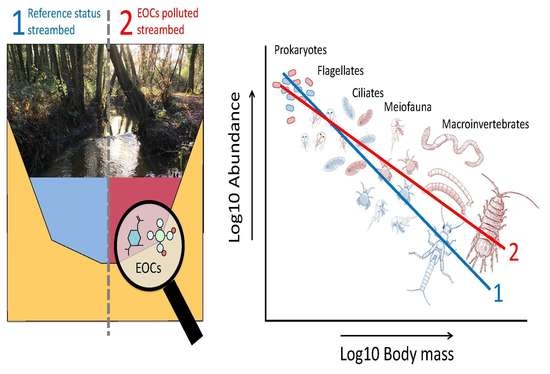
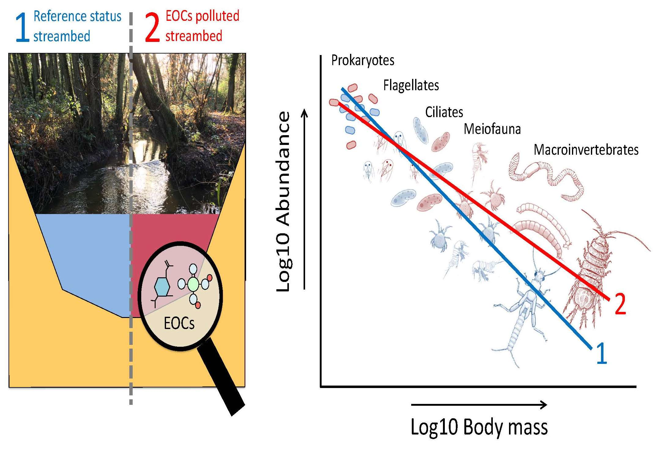
Body size scaling represents a synthetic analytical framework [22] which can be used to integrate the whole streambed assemblage. In particular, the allometric relationship between abundance (N) and body mass (M) is a widely studied pattern in ecological research [23,24]. When individual organisms are grouped into body mass classes, regardless of their taxonomy, the slope of the N–M relationship, or ‘size spectra’, provides an integrated measure of the community structure and the energy flow across trophic levels [25]. This is especially true in freshwater ecosystems, where communities are strongly size-structured [26,27] and gape-limited predation predominates [25]. The intercept of the N–M relationship provides a proxy for the community carrying capacity while the slope represents the energy flow and trophic transference efficiency in the system. Thus, N–M coefficients can be used as a quantitative measure of deviation of a natural community in relation to a reference status due to anthropic stressors [28]. Typically, intercepts decrease and size spectra become steeper under stress conditions [29]. To date, we do not know how EOCs affect the N–M relationship despite the insights that this approach could afford with regard to understanding how EOCs compromise the natural functioning of riverine systems.
Here, we report for the first time the effect of EOC pollution on community composition and N–M relationship coefficients in streambed communities following a regional scale approach. For this purpose, we make use of a large dataset from an existing survey study characterizing streambed communities and environmental features across 30 UK streams [21]. We complement that dataset with unpublished concentrations of 24 model EOCs measured in the pore-space of the streambeds collected at the same temporal and spatial resolution as the community samples. Our study delivers valuable information regarding the presence and concentration of EOCs in natural freshwater systems and their relationship with environmental gradients at a regional scale. Additionally, and exceptionally, these datasets include information of the N and M for individual prokaryotes, unicellular flagellates and ciliates, meiofauna (with body lengths between 0.45 and 500 µm), and macroinvertebrates (body length > 500 µm). Thus, the data comprise more than 10 orders of magnitude in terms of M, ensuring very good representation of the streambed assemblages. We hypothesize that EOC pollution results in detrimental effects to streambed communities, especially for the large-size fractions with lower adaptation capacity to constant exposure to EOCs. Hence, we predict N–M coefficients (intercept and slope) to decrease compared with reference systems. Our findings help understand how EOCs shape the structure, metabolic capacity, and energy flow through components of the streambed assemblage.
2. Methods
2.1. Data Acquisition
Here, we complemented open-access available data from a large survey project (Peralta-Maraver et al. 2019a) with data of EOC concentration, and calculation of N–M relationship coefficients. This dataset comprises 30 streams covering 10 different catchments across England and Wales (UK, Figure 1). Streams varied from small upland, acidic headwaters to large lowland, base-rich chalk streams, covering a large productivity and pollution gradient. Original datasets included information on a large set of environmental variables by study site: canopy cover, sediment morphology (cobbles, gravel, sand, and silt), leaf litter, depth and width of channel, submerged plants and submerged wood, temperature, pH, altitude, latitude, longitude, dissolved organic carbon, ammonium, nitrate, and phosphate [21].
Streambed communities were originally sampled using colonization traps (mesh = 0.5 cm, volume = 38–45 mL) containing three different organic substrates [21]. At each study site, six colonization traps were installed in pairs in the streambed at 0–2 and 15 cm depth for between 29–61 days. After incubation, colonization traps were collected and streambed communities were processed in the laboratory. Sampled organisms were identified and counted (N) and their body dimensions measured. Then, body dimensions (length and width in µm) of all collected individuals were converted into dry carbon content (M) using allometric relationships (further details on sampling design and sample processing are available in Peralta-Maraver et al. [21]).
2.2. Sampling and Processing of EOCs
Streambed pore-water samples were collected from the studied sites using a dive point piezometer during removal of colonization traps. One sampler per stream (n = 30) was pushed vertically into the streambed sediments to a depth of ~7.5 cm and 50 mL of water was pumped manually. Samples were stored in a coolbox at 4 °C and transported to the laboratory within 24 h, where they were frozen until analysis.
EOCs were analyzed using a previously developed direct-injection ultra-high-performance liquid chromatography–tandem mass spectrometry (UHPLC-MS/MS) method (Posselt et al. 2018). A total of 37 polar organic substances (mostly pharmaceuticals and their transformation products) were selected based on their concentration ranges, detection frequency, degradation behavior, and potential persistence, as well as their occurrence on priority lists [12,30,31,32]. Water samples were defrosted and vortexed and a sample volume of 800 μL was combined with 195 μL methanol and 5 μL of an internal standard mix. Afterwards, samples were vortexed again, filtered (Filtropur S 0.45 μm, PES membrane, Sarstedt AG&Co, Nuembrecht, Germany) into LC vials (2 mL, Thermo Scientific, Dreieich, Germany) and analyzed within 12 h. The sample injection volume was 20 μL. Liquid chromatography was performed using a Thermo Scientific Ultimate 3000 UHPLC system equipped with a Waters (Manchester, UK) Acquity UPLC HSS T3 column (1.8 μm, 2.1 mm × 100 mm). The mobile phase consisted of 10 mM acetic acid in deionized water (A) and 10 mM acetic acid in methanol (B). The flow rate was 500 μL min−1 for the gradient and 1000 μL min−1 for column equilibration. Instrumental analysis was carried out using a Thermo Scientific Quantiva triple-quadrupole mass spectrometer equipped with a heated electrospray ionization source. Detailed information on the LC gradient and MS instrument settings can be found in Posselt et al. (2018). A series of calibration standards (in 80% LC/MS grade water/20% MeOH) containing the 37 target compounds and isotopically labelled internal standards was measured three times. Data were processed using the Thermo Scientific Xcalibur 3.1.66.10 instrument software and quantification was performed using the internal standard method. Precision was determined by injecting a quality control standard every 15 samples. The relative standard deviation was <1–12% for all detected compounds except for valsartan acid (21%) and 4-hydroxydiclofenac (20%).
Concentrations in both analyzed blank samples were always below the method limit of quantification for all targets. Method limits of quantification for the 37 targeted compounds are provided in Table S1 and further information regarding materials, chemicals, and standards, as well as additional quality control data can be found elsewhere [12].
2.3. Statistical Analysis
First, a non-metric multidimensional scaling (NMDS) ordination model was applied to compare quantitatively the similarities in profile and concentration (µg L−1) of dissolved compounds (macronutrients and EOCs) across the 30 studied rivers. Excessively large differences between the smallest nonzero and largest concentration values were reduced using the Wisconsin double standardization of variables [33]. This approach improves the detection ability of the similarity index used in NMDS ordination [34]. The Canberra index was used to produce the ordination model and it was run iteratively to find the ordination with the best fit (lower stress value). Subsequently, we evaluated the degree to which the number and concentration of EOCs and dissolved compounds such as nutrients were associated with the ordination axis. For this, we fitted all environmental variables collected originally (Table S1) and new data on profiles and concentrations of EOCs onto the resulting two-dimensional ordination following Peralta-Maraver et al. [35]. Degree correlation and significance of the association between fitted variables and the ordination axis was then assessed after a 1000 randomized permutation test.
Secondly, we applied multiple regression and backward model selection approaches to build the N–M relationship models comparing reference systems (no EOCs detected) with polluted sites (EOCs detected). We pooled data from all colonization traps by study site to provide an integrated sample of the streambed community (n = 30 streambed communities). We constructed the N–M relationship for each site by applying the logarithmic size-binning method [36]. Size bins were determined from the (log10) body mass range for each sampled community and the abundances of organisms were then summed within each size bin [23]. We used a total of six bins to maximize the number of size bins while minimizing the number of empty size bins in the analysis [23,26]. Next, we built a saturated model comparing reference systems with EOC-polluted (two-level factor), and all environmental gradients significantly related with the NMDS ordination. Also, and independently of their relationship with the NMDS ordination, we included pH in the saturated model as a classical driver of the N–M relationship in freshwater systems [37,38]. Covariates were dropped sequentially, and the model re-fitted. Then, the Akaike information criterion (AIC) was applied to select the model with the best fit, and Akaike weights (wi) were used to quantify the relative support of each model in comparison to all alternative models (and therefore Σ wi = 1). In addition, we studied the potential collinear relationship between all covariates included in the candidate models. Model selection and collinearity testing allowed us to inspect potential confounding effects of EOCs with underlying gradients, such as productivity. Model validation was finally applied to verify the underlying assumptions following Zuur et al. [39]. This encompassed testing normality and homoscedasticity of model residuals and their potential dependence with those variables included and not included in the model (e.g., study site).
All statistical analyses were performed using R software (R Core Team, 2019). NMDS ordinations and subsequent variable fitting were carried out using the functions metaMDS and envfit of the R-package Vegan [40].
3. Results
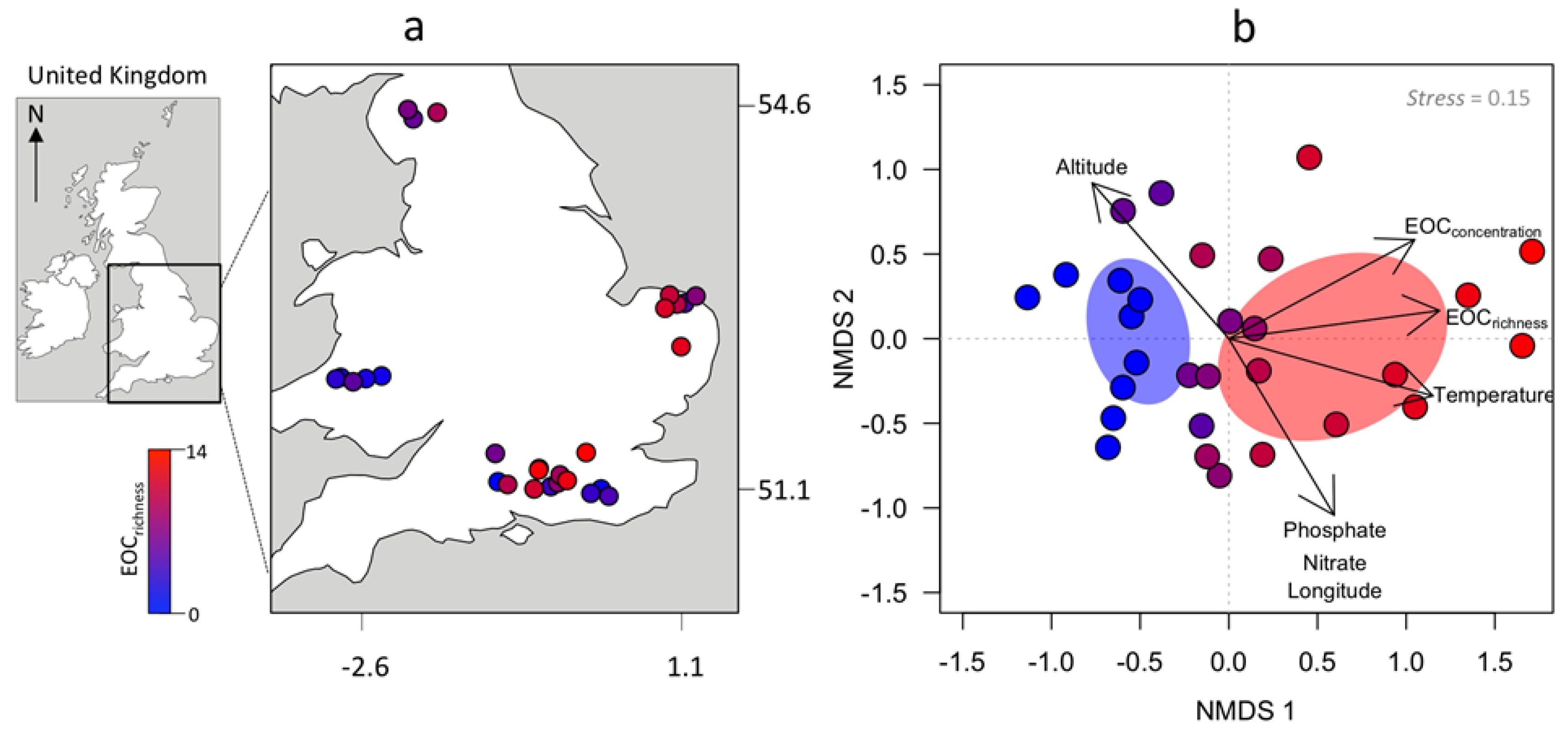
From the 37 targeted compounds, a diverse set of 24 EOCs, including pharmaceuticals and other organic contaminants, were collected from the streambed of two thirds of the study sites (Figure 1, Table 1). The most EOC-polluted sites were mainly distributed in the east and southeast regions of England. The 10 streams unpolluted by EOCs, hereafter called reference sites, were mainly located in the west regions of Wales but were also represented in the southeast of England. The NMDS model based on the 24 EOCs and macronutrients [nitrate, phosphate, and dissolved organic carbon (DOC)] produced a two-dimensional ordination with a very high goodness of fit between the distances in the ordination against the original data (linear fit R2 = 0.995, non-metric fit R2 = 0.990). The resulting ordination (Figure 1b) showed a strong increasing gradient of number of EOCs and concentration positively related with axis 1 (R2 = 0.94, p < 0.01), while dispersion along axis 2 was better explained by the presence and concentration of dissolved nitrate (R2 = 0.94, p < 0.01) and phosphate (R2 = 0.21, p = 0.04), but not DOC (R2 = 0.03, p = 0.62). Environmental fitting onto the ordination showed that number and concentration of EOCs and macronutrients increased significantly along environmental gradients of longitude (R2 = 0.56, p < 0.04) and temperature (R2 = 0.26, p = 0.02), and in the lowland regions of the UK (R2 = 0.58, p < 0.001; Figure 1b).
After model selection routines, all studied variables were excluded from the N–M relationship except EOC pollution in the system (Table 2). The AIC model selection approach suggested a certain improvement of model fitting when adding pH and temperature. However, those variables were also excluded in favor of a model simply comparing reference and polluted sites. AIC and Akaike weight indicate a very strong support of the model including the interaction between M and the EOC pollution (presence/absence of EOCs). This specifies that presence of EOCs in the system strongly determines the intercept and slope of the N–M relationship model. The fitted N–M relationship model including information of the comparison between polluted or reference streams also had a high explanatory capacity (R = 0.67).
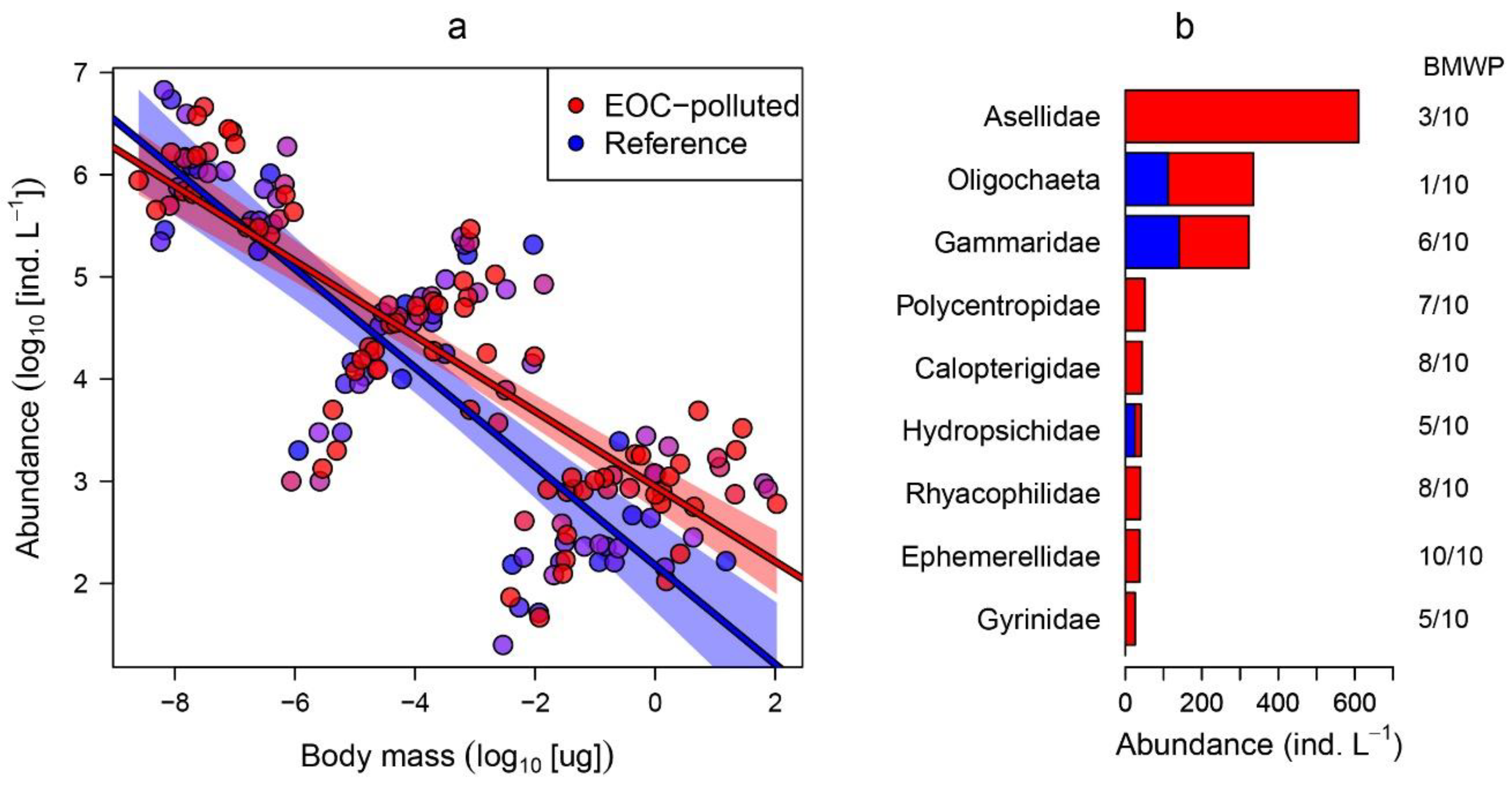
When over more than 10 orders of magnitude in body mass, from flagellates to macroinvertebrates, abundance declined linearly with body mass with an average N–M slope of −0.37 (95% CI = −0.42, −0.31). However, N–M relationship coefficients varied significantly between reference and polluted streams (Table 3). We found that N–M intercepts (as a proxy for community carrying capacity) were higher and size spectra slopes shallower in polluted compared to reference streams. The difference in the 95% CI between fitted regression in the reference and polluted streams became visible in the large size fraction of the N–M relationship, and we attribute this variation to the increase in abundance of the large-size fractions of organisms in polluted sites (Figure 2) which was chiefly associated with increases in pollutant-tolerant groups such as Asellidae and Oligochaeta (Figure 2b).
4. Discussion
In this work, we identified a diverse set of EOCs in streambed sediments across a large regional scale and examined their effect on the size structure of streambed assemblages. We found complex mixtures of EOCs in two thirds of all studied streams, yet we screened our water samples for only 37 target compounds as a small subset of the possible compounds found in natural systems. More than 70,000 daily-use chemicals are registered in the European Union with the potential to enter surface and subsurface water systems [5]. Nevertheless, technical limitations on the detection of EOCs make quantifying and regulating such a variety of chemicals in natural systems unrealistic. Therefore, centering efforts on analyzing carefully selected target chemicals as markers seems to be a suitable strategy to assess the degree of EOC pollution at large spatial scales.
Our findings evidence the strong effect that the presence of EOCs has over the organization of streambed communities, to the point of shielding the effect of other important environmental factors. Temperature, pH, and productivity are considered major drivers in freshwater ecology and determining factors of the size structure and metabolic capacity of streambed communities [26,37,38,41,42]. Even so, both the intercept and size spectra slope of the N–M relationship exhibited higher sensitivity in this work to EOC pollution than to those environmental variables. Hence, the N–M relationship approach seems to be an appropriate analytical and integrative statistical tool for testing deviation of natural communities from a reference status as a consequence of EOC pollution. However, and contrary to our predictions, N–M relationship coefficients increased under polluted conditions. That is, the intercept (i.e., the carrying capacity of the community) increased and the size spectrum slope became shallower. As predicted, the smallest size fractions showed low variation in their abundance when comparing polluted and reference streams. Thus, this pattern is mainly due to the notably higher abundance of certain groups of macroinvertebrates that push up the N–M relationship from the extreme of the mean and largest size fraction. A closer look at the taxa that most influence variation in the N–M relationship (Figure 2) reveals that they mainly belong to tolerant groups of organisms with medium to very low biological monitoring working party scores (BMWP) [43].
The size spectra slope of the M–N relationship describes the rate of biomass depletion through different levels of the food web in freshwater systems, typically becoming shallower as this rate increases [25,26]. Consequently, the existence of more abundant tolerant invertebrates in our study might imply a better transference of biomass and energy between trophic levels and potentially longer food chains. Considering these predictions, we are particularly concerned that several EOCs bioaccumulate untransformed in the cells and tissues of aquatic organisms and even biomagnify through different trophic levels [44,45,46]. Several of the measured EOCs in our survey study, such as diclofenac, ibuprofen, carbamazepine, metoprolol, gemfibrozil, oxazepam, tramadol, and venlafaxine are already known to bioaccumulate in biofilms, invertebrates, and fish in the food webs of stream ecosystems [45,47,48]. In addition, some of these EOCs in larval tissues can be conserved through metamorphosis and adults play the role of a biological vector transporting pharmaceuticals to terrestrial predators [46]. Under our theoretical framework, bioaccumulation is expected to be more acute under a scenario of EOC pollution and the concomitant population increase of tolerant macroinvertebrates. In either case, future experimental approaches are needed to test our prediction. Hence, controlled mesocosm experiments analyzing uptake of EOCs by model organisms and the transference of these EOCs through trophic levels represent a fruitful strategy to assessing these ecological mechanisms. Our metrics involve a broad range of body sizes; however, species-specific responses from different size groups are expected. Therefore, controlled experiments will also shed light on how different populations of taxa will respond to the presence and concentration of different EOCs.
In addition, from the total set of targeted compounds selected as model EOCs, the artificial low-calorie sweetener acesulfame was the most widespread chemical and was detected almost constantly in all polluted streams in our study. This pattern is consistent with previous studies in which acesulfame has been reported as the most ubiquitous EOC in streambed sediments and groundwater across Europe [12,30,31,32,49,50,51]. Thus, our findings strongly support the use of acesulfame as a marker of EOC pollution for application in management and regulation of surface and subsurface waters [49]. Acesulfame is an anthropic source-specific compound released to the environment in high quantities (in quantities of up to 13.8 µg L−1 in this study) and is amenable to rapid and sensitive analysis. It is sufficiently persistent and hydrophilic enough to penetrate into streambed and groundwater systems [49]. In fact, combining analysis of acesulfame with that of acetaminophen (an analgesic pharmaceutical) and sitagliptin (an antihyperglycemic pharmaceutical) allowed us to distinguish between polluted and reference streams in our study.
In summary, in this work we detected strong variation from reference status when comparing N–M relationship coefficients between polluted and reference streams. Even though the ecological mechanisms remain unclear, EOC pollution was associated with an increase in abundance of large-size tolerant macroinvertebrates. This resulted in less size-structured assemblages under polluted conditions with direct implications for the structure of the streambed community and potential biomagnification processes along food webs. With this in mind, future research which characterizes food web structures (feeding links) and quantifies concentrations of EOCs at different trophic levels would be particularly instructive.
Supplementary Materials
The following is available online at https://www.mdpi.com/2073-4441/11/12/2610/s1, Table S1: LC-MS/MS method limits of quantification in µg L–1.
Author Contributions
Conceptualization, I.P.-M. and A.L.R.; methodology, I.P.-M., M.P., D.M.P., A.L.R.; software, I.P.-M.; validation, I.P.-M., D.M.P.; formal analysis, I.P.-M., M.P.; investigation, I.P.-M., M.P., D.M.P., A.L.R.; resources, I.P.-M., M.P., D.M.P., A.L.R.; data curation, I.P.-M., M.P.; writing—original draft preparation, I.P.-M., D.M.P., A.L.R.; writing—review and editing, I.P.-M., M.P., D.M.P., A.L.R.; visualization, I.P.-M., A.L.R.; supervision, A.L.R.; project administration, I.P.-M., A.L.R.; funding acquisition, D.M.P., A.L.R.
Funding
This project was funded by the European Union Horizon 2020 research and innovation programme under Marie Skłodowska-Curie grant agreement No. 641939.
Acknowledgments
The authors thank Jon Benskin and the two anonymous reviewers, who provided useful suggestions that improved the original manuscript.
Conflicts of Interest
No authors have any conflicting interest.
References
- Vörösmarty, C.J.; McIntyre, P.B.; Gessner, M.O.; Dudgeon, D.; Prusevich, A.; Green, P.; Glidden, S.; Bunn, S.E.; Sullivan, C.A.; Liermann, C.R.; et al. Global threats to human water security and river biodiversity. Nature 2010, 467, 555–561. [Google Scholar] [CrossRef] [PubMed]
- Wen, Y.; Schoups, G.; Van De Giesen, N. Organic pollution of rivers: Combined threats of urbanization, livestock farming and global climate change. Sci. Rep. 2017, 7, 43289. [Google Scholar] [CrossRef] [PubMed] [Green Version]
- Malaj, E.; Peter, C.; Grote, M.; Kühne, R.; Mondy, C.P.; Usseglio-Polatera, P. Organic chemicals jeopardize the health of freshwater ecosystems on the continental scale. Proc. Natl. Acad. Sci. USA 2014, 111, 9549–9554. [Google Scholar] [CrossRef] [PubMed] [Green Version]
- Schwarzenbach, R.P.; Escher, B.I.; Fenner, K.; Hofstetter, T.B.; Johnson, C.A.; Von Gunten, U.; Wehrli, B. The challenge of micropollutants in aquatic systems. Science 2006, 313, 1072–1077. [Google Scholar] [CrossRef] [PubMed]
- Reemtsma, T.; Weiss, S.; Mueller, J.; Petrovic, M.; González, S.; Barcelo, D.; Ventura, F.; Knepper, T.P. Polar pollutants entry into the water cycle by municipal wastewater: A European perspective. Environ. Sci. Technol. 2006, 40, 5451–5458. [Google Scholar] [CrossRef] [PubMed]
- Pal, A.; Gin, K.Y.H.; Lin, A.Y.C.; Reinhard, M. Impacts of emerging organic contaminants on freshwater resources: Review of recent occurrences, sources, fate and effects. Sci. Total Environ. 2010, 408, 6062–6069. [Google Scholar] [CrossRef] [PubMed]
- Kidd, K.A.; Blanchfield, P.J.; Mills, K.H.; Palace, V.P.; Evans, R.E.; Lazorchak, J.M.; Flick, R.W. Collapse of a fish population after exposure to a synthetic estrogen. Proc. Natl. Acad. Sci. USA 2007, 104, 8897–8901. [Google Scholar] [CrossRef] [Green Version]
- Galus, M.; Rangarajan, S.; Lai, A.; Shaya, L.; Balshine, S.; Wilson, J.Y. Effects of chronic, parental pharmaceutical exposure on zebrafish (Danio rerio) offspring. Aquat. Toxicol. 2014, 151, 124–134. [Google Scholar] [CrossRef]
- Stamm, C.; Räsänen, K.; Burdon, F.J.; Altermatt, F.; Jokela, J.; Joss, A.; Ackermann, M.; Eggen, R.I. Unravelling the impacts of micropollutants in aquatic ecosystems: Interdisciplinary studies at the interface of large-scale ecology. Adv. Ecol. Res. 2016, 55, 183–223. [Google Scholar]
- Kubec, J.; Hossain, S.; Grabicová, K.; Randák, T.; Kouba, A.; Grabic, R.; Roje, S.; Buřič, M. Oxazepam alters the behavior of crayfish at diluted concentrations, venlafaxine does not. Water 2019, 11, 196. [Google Scholar] [CrossRef] [Green Version]
- Lewandowski, J.; Arnon, S.; Banks, E.; Batelaan, O.; Betterle, A.; Broecker, T.; Coll, C.; Drummond, J.D.; Garcia, J.G.; Galloway, J.; et al. Is the Hyporheic Zone Relevant beyond the Scientific Community? Water 2019, 11, 2230. [Google Scholar] [CrossRef] [Green Version]
- Posselt, M.; Jaeger, A.; Schaper, J.L.; Radke, M.; Benskin, J.P. Determination of polar organic micropollutants in surface and pore water by high-resolution sampling-direct injection-ultra high performance liquid chromatography-tandem mass spectrometry. Environ. Sci. Process. Impacts 2018, 20, 1716–1727. [Google Scholar] [CrossRef] [PubMed] [Green Version]
- Richmond, E.K.; Grace, M.R.; Kelly, J.J.; Reisinger, A.J.; Rosi, E.J.; Walters, D.M. Pharmaceuticals and personal care products (PPCPs) are ecological disrupting compounds (EcoDC). Elem. Sci. Anth. 2017, 5, 66. [Google Scholar] [CrossRef] [Green Version]
- Findlay, S. Importance of surface-subsurface exchange in stream ecosystems: The hyporheic zone. Limnol. Oceanogr. 1995, 40, 159–164. [Google Scholar] [CrossRef]
- Hester, E.T.; Young, K.I.; Widdowson, M.A. Mixing of surface and groundwater induced by riverbed dunes: Implications for hyporheic zone definitions and pollutant reactions. Water Resour. Res. 2013, 49, 5221–5237. [Google Scholar] [CrossRef]
- Subirats, J.; Triadó-Margarit, X.; Mandaric, L.; Acuña, V.; Balcázar, J.L.; Sabater, S.; Borrego, C.M. Wastewater pollution differently affects the antibiotic resistance gene pool and biofilm bacterial communities across streambed compartments. Mol. Ecol. 2017, 26, 5567–5581. [Google Scholar] [CrossRef] [Green Version]
- Subirats, J.; Timoner, X.; Sànchez-Melsió, A.; Balcázar, J.L.; Acuña, V.; Sabater, S.; Borrego, C.M. Emerging contaminants and nutrients synergistically affect the spread of class 1 integron-integrase (intI1) and sul1 genes within stable streambed bacterial communities. Water Res. 2018, 138, 77–85. [Google Scholar] [CrossRef]
- Láng, J.; Kőhidai, L. Effects of the aquatic contaminant human pharmaceuticals and their mixtures on the proliferation and migratory responses of the bioindicator freshwater ciliate Tetrahymena. Chemosphere 2012, 89, 592–601. [Google Scholar] [CrossRef]
- Althakafy, J.T.; Kulsing, C.; Grace, M.R.; Marriott, P.J. Determination of selected emerging contaminants in freshwater invertebrates using a universal extraction technique and liquid chromatography accurate mass spectrometry. J. Sep. Sci. 2018, 41, 3706–3715. [Google Scholar] [CrossRef]
- Miller, T.H.; Ng, K.T.; Bury, S.T.; Bury, S.E.; Bury, N.R.; Barron, L.P. Biomonitoring of pesticides, pharmaceuticals and illicit drugs in a freshwater invertebrate to estimate toxic or effect pressure. Environ. Int. 2019, 129, 595–606. [Google Scholar] [CrossRef]
- Peralta-Maraver, I.; Perkins, D.M.; Thompson, M.S.; Fussmann, K.; Reiss, J.; Robertson, A.L. Comparing biotic drivers of litter breakdown across stream compartments. J. An. Ecol. 2019, 88, 1146–1157. [Google Scholar] [CrossRef] [PubMed]
- Brown, J.H.; Gillooly, J.F.; Allen, A.P.; Savage, V.M.; West, G.B. Toward a metabolic theory of ecology. Ecology 2004, 85, 1771–1789. [Google Scholar] [CrossRef]
- White, E.P.; Ernest, S.M.; Kerkhoff, A.J.; Enquist, B.J. Relationships between body size and abundance in ecology. Trends Ecol. Evol. 2007, 22, 323–330. [Google Scholar] [CrossRef] [PubMed] [Green Version]
- Trebilco, R.; Baum, J.K.; Salomon, A.K.; Dulvy, N.K. Ecosystem ecology: Size-based constraints on the pyramids of life. Trends Ecol. Evol. 2013, 28, 423–431. [Google Scholar] [CrossRef]
- Kerr, S.R.; Dickie, L.M. The Biomass Spectrum: A PredatorPrey Theory of Aquatic Production; Columbia University Press: Chichester, NY, USA, 2001. [Google Scholar]
- Perkins, D.M.; Durance, I.; Edwards, F.K.; Grey, J.; Hildrew, A.G.; Jackson, M.; Jones, J.I.; Lauridsen, R.B.; Layer-Dobra, K.; Thompson, M.S.; et al. Bending the rules: Exploitation of allochthonous resources by a top-predator modifies size-abundance scaling in stream food webs. Ecol. Lett. 2018, 21, 1771–1780. [Google Scholar] [CrossRef] [Green Version]
- Peralta-Maraver, I.; Robertson, A.L.; Perkins, D.M. Depth and vertical hydrodynamics constrain the size structure of a lowland streambed community. Biol. Lett. 2019, 15, 20190317. [Google Scholar] [CrossRef] [Green Version]
- Petchey, O.L.; Morin, P.J.; Hulot, F.D. Contributions of aquatic model systems to our understanding of biodiversity and ecosystem functioning. In Biodiversity and Ecosystem Functioning—Synthesis and Perspectives; Loreau, M., Naeem, S., Inchausti, P., Eds.; Oxford University Press: Oxford, UK, 2002; pp. 127–138. [Google Scholar]
- Petchey, O.L.; Belgrano, A. Body-size distributions and size-spectra: Universal indicators of ecological status? Biol. Lett. 2010, 6, 434–437. [Google Scholar] [CrossRef] [Green Version]
- Li, Z.; Sobek, A.; Radke, M. Fate of pharmaceuticals and their transformation products in four small European rivers receiving treated wastewater. Environ. Sci. Technol. 2016, 50, 5614–5621. [Google Scholar] [CrossRef] [Green Version]
- Schaper, J.L.; Posselt, M.; Bouchez, C.; Jaeger, A.; Nuetzmann, G.; Putschew, A.; Singer, G.; Lewandowski, J. Fate of Trace Organic Compounds in the Hyporheic Zone: Influence of Retardation, the Benthic Biolayer, and Organic Carbon. Environ. Sci. Technol. 2019, 53, 4224–4234. [Google Scholar] [CrossRef]
- Mechelke, J.; Vermeirssen, E.L.; Hollender, J. Passive sampling of organic contaminants across the water-sediment interface of an urban stream. Water Res. 2019, 165, 114966. [Google Scholar] [CrossRef] [Green Version]
- Bray, J.R.; Curtis, J.T. An ordination of the upland forest communities of southern Wisconsin. Ecol. Monogr. 1957, 27, 325–349. [Google Scholar] [CrossRef]
- Oksanen, J. Multivariate Analysis of Ecological Communities in R: Vegan Tutorial. 2015. Available online: http://cc.oulu.fi/~jarioksa/opetus/metodi/veg-antutor.pdf (accessed on 19 November 2019).
- Peralta-Maraver, I.; Robertson, A.L.; Rezende, E.L.; Lemes da Silva, A.L.; Tonetta, D.; Lopes, M.; Schmitt, R.; Leite, N.K.; Nuñer, A.; Petrucio, M.M. Winter is coming: Food web structure and seasonality in a subtropical freshwater coastal lake. Ecol. Evol. 2017, 7, 4534–4542. [Google Scholar] [CrossRef] [PubMed] [Green Version]
- Edwards, A.M.; Robinson, J.P.; Plank, M.J.; Baum, J.K.; Blanchard, J.L. Testing and recommending methods for fitting size spectra to data. Methods Ecol. Evol. 2017, 8, 57–67. [Google Scholar] [CrossRef]
- Mulder, C.; Elser, J.J. Soil acidity, ecological stoichiometry and allometric scaling in grassland food webs. Glob. Chang. Biol. 2009, 15, 2730–2738. [Google Scholar] [CrossRef] [Green Version]
- Layer, K.; Riede, J.O.; Hildrew, A.G.; Woodward, G. Food web structure and stability in 20 streams across a wide ph gradient. Adv. Ecol. Res. 2010, 42, 265–299. [Google Scholar]
- Zuur, A.F.; Ieno, E.N.; Walker, N.J.; Savaliev, A.A.; Smith, G.M. Mixed Effects Models and Extensions in Ecology with R; Springer: New York, NY, USA, 2009; p. 57. [Google Scholar]
- Oksanen, J.; Blanchet, F.G.; Kindt, R.; Legendre, P.; Minchin, P.R.; O’Hara, R.B.; Simpson, G.L.; Solymos, P.; Stevens, M.H.H.; Wagner, H. Vegan: Community Ecology Package. R Package Version 2.0–10. 2013. Available online: http://CRAN.R–project.org/ package=vegan (accessed on 7 November 2019).
- Dossena, M.; Yvon-Durocher, G.; Grey, J.; Montoya, J.M.; Perkins, D.M.; Trimmer, M.; Woodward, G. Warming alters community size structure and ecosystem functioning. Proc. Biol. Sci. Replaces Proc. R. Soc. 2012, 279, 3011–3019. [Google Scholar] [CrossRef] [Green Version]
- O’Gorman, E.J.; Pichler, D.E.; Adams, G.; Benstead, J.P.; Cohen, H.; Craig, N.; Cross, W.F.; Demars, B.O.; Friberg, N.; Gislason, G.M.; et al. Impacts of warming on the structure and functioning of aquatic communities: Individual-to ecosystem-level responses. Adv. Ecol. Res. 2012, 47, 81–176. [Google Scholar]
- Hawkes, H.A. Origin and development of the biological monitoring working party score system. Water Res. 1998, 32, 964–968. [Google Scholar] [CrossRef]
- Zenker, A.; Cicero, M.R.; Prestinaci, F.; Bottoni, P.; Carere, M. Bioaccumulation and biomagnification potential of pharmaceuticals with a focus to the aquatic environment. J. Environ. Manag. 2014, 133, 378–387. [Google Scholar] [CrossRef]
- Ruhí, A.; Acuña, V.; Barceló, D.; Huerta, B.; Mor, J.R.; Rodríguez-Mozaz, S.; Sabater, S. Bioaccumulation and trophic magnification of pharmaceuticals and endocrine disruptors in a Mediterranean river food web. Sci. Total Environ. 2016, 540, 250–259. [Google Scholar] [CrossRef]
- Richmond, E.K.; Rosi, E.J.; Walters, D.M.; Fick, J.; Hamilton, S.K.; Brodin, T.; Sundelin, A.; Grace, M.R. A diverse suite of pharmaceuticals contaminates stream and riparian food webs. Nat. Commun. 2019, 9, 4491. [Google Scholar] [CrossRef] [PubMed] [Green Version]
- Brown, J.N.; Paxéus, N.; Förlin, L.; Larsson, D.J. Variations in bioconcentration of human pharmaceuticals from sewage effluents into fish blood plasma. Environ. Toxicol. Pharmacol. 2007, 24, 267–274. [Google Scholar] [CrossRef] [PubMed]
- Fick, J.; Lindberg, R.H.; Tysklind, M.; Larsson, D.J. Predicted critical environmental concentrations for 500 pharmaceuticals. Regul. Toxicol. Pharmacol. 2010, 58, 516–523. [Google Scholar] [CrossRef] [PubMed]
- Buerge, I.J.; Buser, H.-R.; Kahle, M.; Müller, M.D.; Poiger, T. Ubiquitous occurrence of the artificial sweetener acesulfame in the aquatic environment: An ideal chemical marker of domestic wastewater in groundwater. Environ. Sci. Technol. 2009, 43, 4381–4385. [Google Scholar] [CrossRef] [PubMed]
- Jaeger, A.; Posselt, M.; Betterle, A.; Schaper, J.; Mechelke, J.; Coll, C.; Lewandowski, J. Spatial and Temporal Variability in Attenuation of Polar Organic Micropollutants in an Urban Lowland Stream. Environ. Sci. Technol. 2019, 53, 2383–2395. [Google Scholar] [CrossRef] [Green Version]
- Jaeger, A.; Coll, C.; Posselt, M.; Mechelke, J.; Rutere, C.; Betterle, A.; Raza, M.; Mehrtens, A.; Meinikmann, K.; Portmann, A.; et al. Using recirculating flumes and a response surface model to investigate the role of hyporheic exchange and bacterial diversity on micropollutant. Environ. Sci. Process. Impacts 2019, 21. [Google Scholar] [CrossRef] [Green Version]
Figure 1.
(a) Locations of the study systems in the United Kingdom, including number of emerging organic contaminants (EOCrichness). (b) Non-metric multidimensional scaling (NMDS) ordination model based on Canberra index comparing the dissimilarities in profile and concentration (µg L−1) of dissolved compounds (macronutrients and EOCs) across the 30 studied rivers. Environmental gradients that were significantly correlated (p < 0.05) with the ordination are overlapped with the ordination. The arrows depict the relationship of fitted variables with the ordination.

Figure 2.
(a) Results from the linear regression of log10 total abundance on log10 body mass bin (N–M relationship) comparing EOC-polluted and reference streams. Each data point denotes the abundance of a given size class for each sampling unit. The fitted lines represent the average N–M slope for EOC-polluted and reference streams. (b) Abundance and biological monitoring working party (BMWP) score of the macroinvertebrate families belonging to the largest size bin across the studied EOC-polluted and reference streams.


Table 1.
Concentration (µg L−1) of the target EOCs analyzed across the 30 studied streams: 1H-benzotriazole (1.H.B.), 2/4-chlorobenzoic acid (C.Acid), 4-hydroxydiclofenac (4.H.D.), acesulfame (Acesu), acetaminophen (Aceta), carbamazepine (Carba), clofibric acid (C.Acid2), diclofenac (Diclo), 11-dihydroxy carbamazepine (11.D.C), furosemide (Furo), gemfibrozil (Gem), guanylurea (Guan), ibuprofen (Ibu), metformin (Metf), metoprolol acid (M.Acid), metoprolol (Meto), naproxen (Napro), O-desmethylvenlafaxine (O.Des), oxazepam (Oxa), propranolol (Prop), sitagliptin (Sita), sotalol (Sota), tramadol (Trama), and venlafaxine (Venl). Table shows latitude (Lat) and longitude (Lon) and total amount of EOCs of studied streams.
| River | Lat | Lon | Acesu | Aceta | Sita | O.Des | 11.D.C. | Napro | Guan | Metf | Venl | M.Acid | Carba | Oxa | Prop | Sota | 4.H.D. | Trama | Diclo | 1.H.B. | Ibu | 11.D.C. | C.Acid2 | Furo | Meto | Gem | Tot EOCs |
|---|---|---|---|---|---|---|---|---|---|---|---|---|---|---|---|---|---|---|---|---|---|---|---|---|---|---|---|
| Beverly Brooks | 51.44 | 0.25 | 13.8 | 0.1 | 0.4 | 1.1 | 44.8 | 1.5 | 0.6 | 0.6 | 0.2 | 0.6 | 0.1 | 0.2 | 2.9 | 0.6 | 14 | ||||||||||
| Loddon | 51.42 | 1.72 | 0.8 | 0.1 | 0.4 | 0.8 | 9.7 | 0.2 | 0.2 | 0.1 | 0.2 | 0.7 | 0.1 | 0.4 | 0.1 | 13 | |||||||||||
| Wey | 51.19 | 0.68 | 0.8 | 0.5 | 0.1 | 0.1 | 0.7 | 5.2 | 0.4 | 0.1 | 0.8 | 0.3 | 0.2 | 0.6 | 12 | ||||||||||||
| Waveney | 52.42 | 1.36 | 0.5 | 0.1 | 0.6 | 0.2 | 1.7 | 0.4 | 0.2 | 0.3 | 0.1 | 9 | |||||||||||||||
| Wensum | 52.42 | 1.36 | 0.2 | 0.4 | 0.3 | 0.4 | 0.4 | 0.8 | 0.2 | 0.3 | 8 | ||||||||||||||||
| Deadwater | 51.17 | 0.85 | 1.9 | 0.2 | 0.7 | 0.1 | 0.7 | 0.1 | 6 | ||||||||||||||||||
| Stiffkey | 52.92 | 0.89 | 0.3 | 0.2 | 0.2 | 0.2 | 0.1 | 5 | |||||||||||||||||||
| Tat | 52.82 | 0.75 | 0.5 | 0.9 | 0.2 | 0.9 | 4 | ||||||||||||||||||||
| River Leith | 54.61 | −2.62 | 0.5 | 0.4 | 0.4 | 3 | |||||||||||||||||||||
| Nadder | 51.12 | 0.90 | 1.7 | 0.4 | 0.1 | 3 | |||||||||||||||||||||
| Test | 51.14 | 1.47 | 1.0 | 0.2 | 0.4 | 3 | |||||||||||||||||||||
| Glaven | 52.93 | 1.63 | 0.2 | 0.7 | 0.4 | 3 | |||||||||||||||||||||
| Lamports | 51.15 | 1.72 | 0.1 | 0.3 | 0.1 | 3 | |||||||||||||||||||||
| Lyde | 51.29 | 1.72 | 0.2 | 0.8 | 0.2 | 3 | |||||||||||||||||||||
| GI1 | 52.14 | −3.84 | 0.4 | 0.1 | 2 | ||||||||||||||||||||||
| Howe Beck | 54.68 | −2.59 | 0.1 | 0.7 | 2 | ||||||||||||||||||||||
| Bure | 52.82 | 1.21 | 0.1 | 0.1 | 2 | ||||||||||||||||||||||
| River Crowdundle | 51.15 | 1.72 | 0.1 | 0.1 | 2 | ||||||||||||||||||||||
| Kennet | 51.42 | 1.72 | 0.2 | 0.7 | 2 | ||||||||||||||||||||||
| River Lyvennet | 54.68 | −2.61 | 0.1 | 0.5 | 2 | ||||||||||||||||||||||
| LI7 | 52.13 | −3.75 | 0 | ||||||||||||||||||||||||
| LI8 | 52.16 | −3.75 | 0 | ||||||||||||||||||||||||
| LI3 | 52.14 | −3.73 | 0 | ||||||||||||||||||||||||
| Old Lodge | 54.65 | −2.64 | 0 | ||||||||||||||||||||||||
| Lone Oak | 51.77 | 0.13 | 0 | ||||||||||||||||||||||||
| LI6 | 51.44 | 0.25 | 0 | ||||||||||||||||||||||||
| Broadstone Stream | 51.89 | 0.57 | 0 | ||||||||||||||||||||||||
| Oakhanger | 51.45 | 0.79 | 0 | ||||||||||||||||||||||||
| Anton | 51.15 | 1.46 | 0 | ||||||||||||||||||||||||
| Morland Beck | 51.23 | 1.72 | 0 |
Table 2.
Comparison of the regression models testing EOC pollution, pH, temperature (Temp), longitude (Lon), altitude (alt), nitrate (Nit), and phosphate (Phos) on the abundance–body mass (N–M) relationship (all models include an intercept, which has not been shown for simplicity). Legend: AIC, Akaike information criterion; LogLik, maximum likelihood estimator; wi, Akaike weight. Candidate model with the best fit is highlighted in bold.
| Response | Predictors | N | AIC | ΔAIC | LogLik | wi |
|---|---|---|---|---|---|---|
| Log 10 (N) | log10(M) × EOCs + pH + Temp + Lon + Lat + Alt + Nit + Phos | 12 | 403.82 | 9.23 | 0.01 | 0.00 |
| log10(M) × EOCs + pH + Temp + Lon + Lat + Alt + Nit | 11 | 402.30 | 7.70 | 0.02 | 0.01 | |
| log10(M) × EOCs + pH + Temp + Lon + Lat + Alt | 10 | 402.35 | 7.75 | 0.02 | 0.01 | |
| log10(M) × EOCs + pH + Temp + Lon + Lat | 9 | 401.17 | 6.57 | 0.04 | 0.02 | |
| log10(M) × EOCs + pH + Temp + Lon | 8 | 399.18 | 4.59 | 0.10 | 0.05 | |
| log10(M) × EOCs + pH + Temp | 7 | 397.32 | 2.72 | 0.26 | 0.12 | |
| log10(M) × EOCs + pH | 6 | 396.15 | 1.55 | 0.46 | 0.22 | |
| log10(M) × EOCs | 5 | 394.60 | 0.00 | 1.00 | 0.47 | |
| log10(M) + EOCs | 4 | 397.88 | 3.28 | 0.19 | 0.09 | |
| log10(M) | 3 | 401.22 | 6.62 | 0.04 | 0.02 |
Table 3.
Summary table of the fitted abundance–body mass regression (fixed coefficients). Fixed coefficients (Coef), standard errors (SE), degrees of freedom (DF), t values, and p values (p) are given. Significance codes (Sig): 0 (***), 0.01 (*).
Table 3.
Summary table of the fitted abundance–body mass regression (fixed coefficients). Fixed coefficients (Coef), standard errors (SE), degrees of freedom (DF), t values, and p values (p) are given. Significance codes (Sig): 0 (***), 0.01 (*).
| Fixed Equation Terms | Coef | SE | t Value | p Value | Sig |
|---|---|---|---|---|---|
| Intercept | 2.95 | 0.12 | 25.20 | > 0.001 | *** |
| Log10 body mass | −0.37 | 0.03 | −13.87 | > 0.001 | *** |
| Presence/absence of EOCs | −0.77 | 0.24 | −3.22 | 0.001 | *** |
| Log10 body mass * EOC pollution | −0.12 | 0.05 | 0.05 | 0.02 | * |
© 2019 by the authors. Licensee MDPI, Basel, Switzerland. This article is an open access article distributed under the terms and conditions of the Creative Commons Attribution (CC BY) license (http://creativecommons.org/licenses/by/4.0/).
Share and Cite
MDPI and ACS Style
Peralta-Maraver, I.; Posselt, M.; Perkins, D.M.; Robertson, A.L. Mapping Micro-Pollutants and Their Impacts on the Size Structure of Streambed Communities. Water 2019, 11, 2610. https://doi.org/10.3390/w11122610
AMA Style
Peralta-Maraver I, Posselt M, Perkins DM, Robertson AL. Mapping Micro-Pollutants and Their Impacts on the Size Structure of Streambed Communities. Water. 2019; 11(12):2610. https://doi.org/10.3390/w11122610
Chicago/Turabian StylePeralta-Maraver, Ignacio, Malte Posselt, Daniel M. Perkins, and Anne L. Robertson. 2019. "Mapping Micro-Pollutants and Their Impacts on the Size Structure of Streambed Communities" Water 11, no. 12: 2610. https://doi.org/10.3390/w11122610
Note that from the first issue of 2016, this journal uses article numbers instead of page numbers. See further details here.