Numerical Analysis of Woltman Meter Accuracy under Flow Perturbations

Abstract

One of the unknowns in the instrumentation for water measurement is what degree of influence other hydraulic elements exert on the velocity profile and, consequently, on the measurement errors. In this work, the measurement errors of a horizontal-axis Woltman meter produced by a gate valve and by a butterfly valve in different hydraulic configurations were studied using a simplified numerical model. The gate valve was installed beside the meter and three pipe diameters upstream of the meter and were operated with closures of 75%, 50% and 25%, while the butterfly valve was installed at three pipe diameters upstream of the meter with closures of 0° (open) and 30°. The numerical model based on the rotor’s torque balance equations and Computational Fluid Dynamics (CFD) was validated by experimental tests. According to the results, it was concluded that the proposed model is valid and capable of estimating the errors caused by the hydraulic fittings arranged next to the meter. In addition, it is evident that for the analysed operating range, both valves must be installed at least three diameters of straight pipe upstream of the meter.

1. Introduction

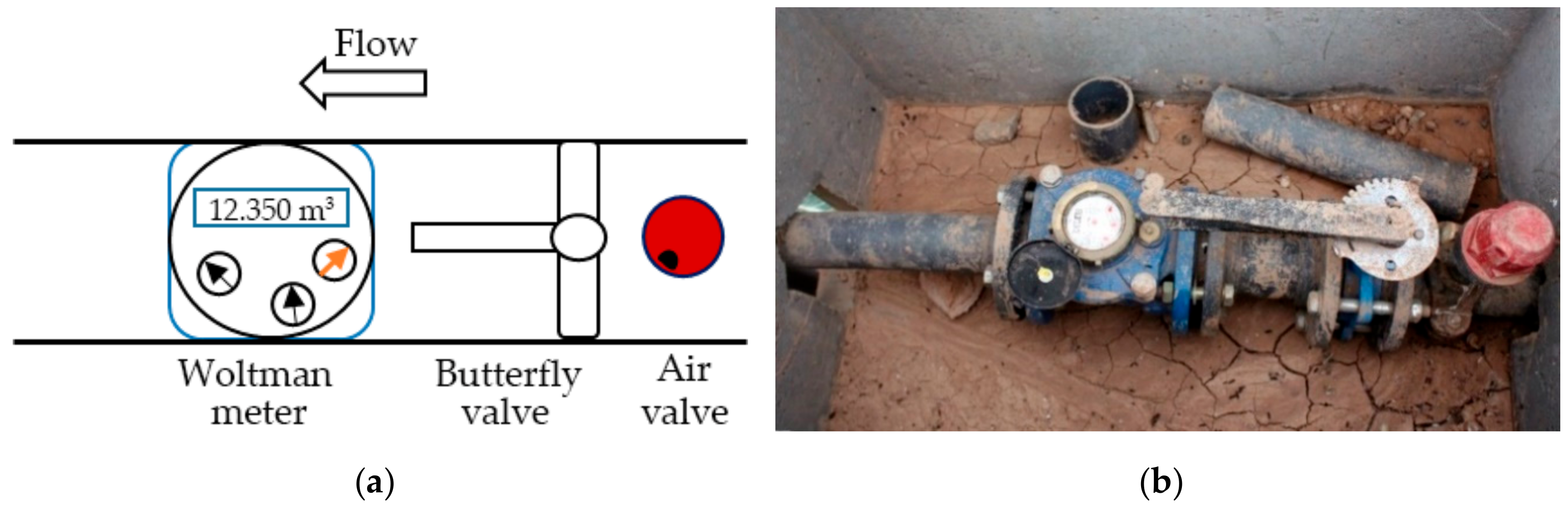
Commonly, Woltman water meters are used in pressurized facilities, such as pumping stations, distribution networks and filtration systems, for measuring water consumption in irrigation networks [1,2]. This equipment integrates water flow rate over a period of time to register total water consumption. However, sometimes volume measurement problems are caused by inconvenient meter installation (Figure 1).

An internal multi-bladed turbine or rotor is the main element of this device and can be disposed with a horizontal or vertical axis. The rotational speed of the turbine is directly proportional to the volumetric flow rate measured. This velocity depends on the construction characteristics, the flow incidence angle and the impact velocity of the water passing through the rotor [3]. Thus, a fully developed velocity profile will result in an axial symmetry distribution of driving forces around the turbine, generating calibrated and accurate measurements.

Distorted velocity profiles and swirls, normally caused by hydraulic fittings close to the meter, can induce significant measurement errors [4]. Each hydraulic element can disturb the flow in different ways. Thus, the recommended manufacturer installation distance varies with the type of hydraulic accessory placed in the pipe [5]. Even when following the constraints recommended by manufacturers, irregular measurements can be found in the field [6].

Thus, detailed study of the influence on measurement errors is essential to reduce them to an acceptable value and to define the lengths of the straight pipe upstream of the meter. This type of study, usually conducted via experimentation [7], can be modelled through computational simulation techniques [8,9,10,11].

Multiple studies have used Computational Fluid Dynamics (CFD) as a simulation tool for hydraulic element design or flow behaviour analysis [12,13,14,15]. Other technologies such as ultrasonic [9,16,17,18], electromagnetic [18,19,20] or multi-hole orifice [21] flow meter have been simulated to analyse the influences of upstream perturbations. Despite its wide use, even with other hydraulic accessories and water meters [20,22,23,24], research on precision of Woltman meters operating with hydraulic flow regulating elements, such as gate and butterfly valves, is scarce.

Some studies have validated CFD techniques to simulate the operation of water meters [16,25] and correspondingly, the influence of hydraulic fittings [8,26] or other structures [27] on the distortion of the measured flow. The use of CFD numerical models can effectively reduce the high cost of experimental testing with turbine flowmeters [28].

Hence, this research analysed the flow perturbations generated by a gate and a butterfly valve installed near the water meter at a 0D and 3D distance, in which D stands for the diameter of the meter. In particular, theoretical equations of hydrodynamics with CFD simulations were combined to construct a simplified and validated numerical model. The proposed numerical model was used to consider the effect of distorted flow on meter accuracy.

2. Materials and Methods

2.1. Theoretical Analysis

In the initial part of the study, a hydrodynamic analysis of water was performed to understand how flow disturbances affect the measurement of the instrument. Specifically, the operating principle and theoretical equations were set out to estimate the driving torque and measurement error used for the numerical analysis.

2.2. Computational Simulation

In the second part of the research, the CFD model was developed to obtain velocity profiles at different points of the pipe section. The CFD simulations were carried out with FLUENT 6.1 software in three phases: pre-processed, processed and post-processed.

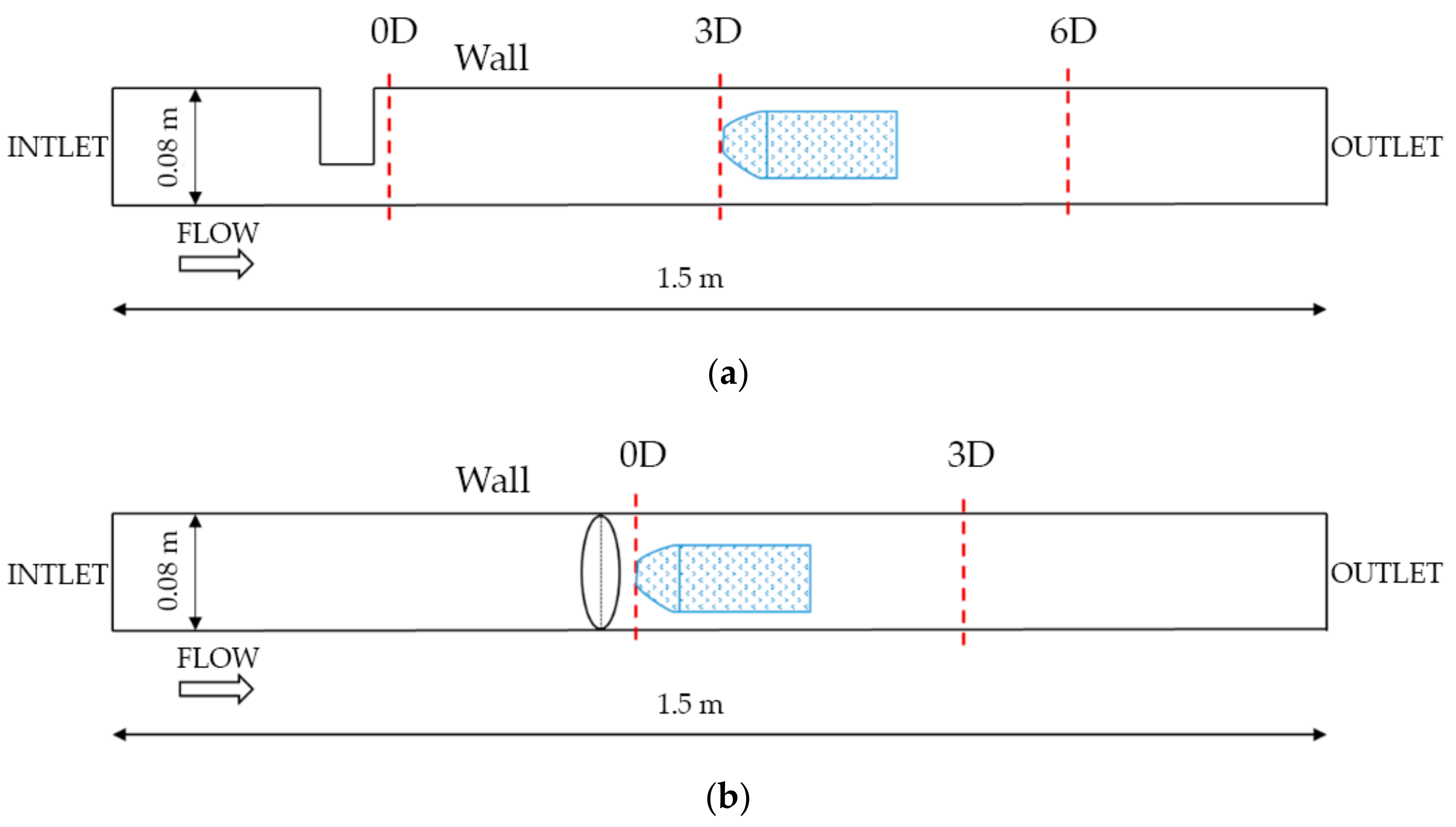
In the pre-processing phase, the tri-dimensional (3D) geometry of the stationary components and the meshing of the computational domain with the GAMBIT^© graphic interface was created Figure 2.

Particularly, the meter and hydraulic elements were characterised and the mesh and its refinement were generated. Before processing, fluid properties and boundary conditions were defined for each case. Inlet velocity and pressure at the outlet were the boundary conditions chosen for the inlet and outlet pipe flow characteristics, respectively (

Table 1. Study cases and boundary conditions for the numerical simulation of a horizontal-axis Woltman meter.

Cases Studied
Configuration	Reference	Gate Valve			Butterfly Valve
Opening degree	-	75% closed	50% closed	25% closed	open	30° closed
Distance	-	0D, 3D	0D, 3D	0D, 3D	3D	3D
Boundary conditions
Input velocity (m s−1)	1, 2, 3, 4, 6	1, 2, 3, 4, 6	1, 2, 3, 4, 6	1, 2, 3, 4, 6	1, 2, 3, 4, 6	1, 2, 3, 4, 6
Outlet pressure (bar)	3	3	3	3	3	3
Wall condition k (mm)	0.1	0.1	0.1	0.1	0.1	0.1
Symmetry wall	yes	yes	yes	yes	no	no

D: Pipe diameter.

).

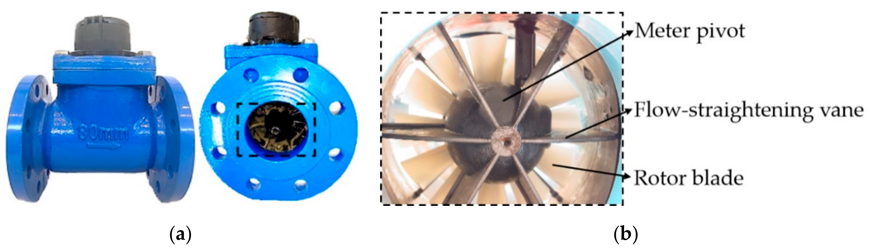
The modelled hydraulic device was a horizontal-axis Woltman meter. To simplify the computational processing time, only fixed internal elements of the device were analysed. The internal geometry consisted of a meter pivot and six flow-straightening vanes (Figure 3).

The study was conducted for three different hydraulic configurations. The first, or reference case, considered the meter installation with a fully developed velocity profile due to the installation of sufficient straight-pipe length upstream. The second and third configurations simulated the installation of a gate and butterfly valve, respectively, with different degrees of closure and distances to the meter. All the hydraulic elements had a nominal diameter (DN) of 80 mm.

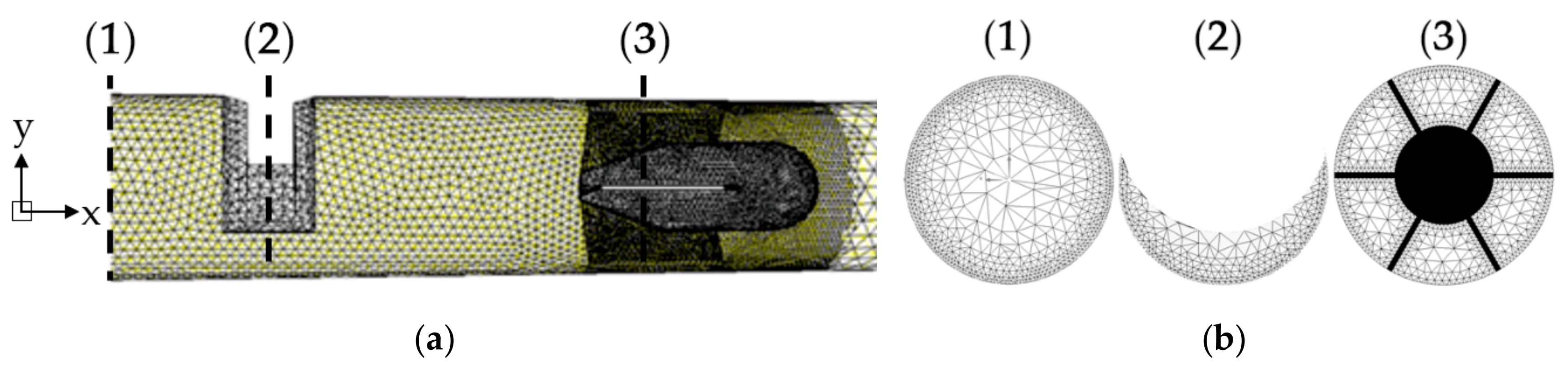
Mesh was created with the discretization of the computational domains described in control volumes or asymmetric cells of 1 mm (Figure 4).

Refinement was done with the Hanging Node technique, which adds a new knot to the edge formed by two vertices so that the marked cells are subdivided approximately at twice the number of edges of the cell. This resulted in an optimal unstructured mesh [29] with double refining in areas with high variations in velocity or pressure. The total number of cells in the grid was in between 354,643 and 456,458, depending on the simulation studied.

In simulations with a symmetric configuration, such as the reference case and the gate valve, only half of the pipeline was evaluated to accelerate the computational calculations.

In the CFD numerical processing phase, the finite element method was used to discretize differential equations in control volumes or cells. These equations were approximated with the technique of finite differences and, subsequently, by means of mathematical algorithms of the iterative-calculation-type Semi-Implicit Method for Pressure-Linked Equations, and a coherent union between pressures and velocities was established.

Mass conservation and Reynolds Average Navier–Stokes (RANS) with a turbulent Standard k-ε model was used as governing flow equations. A numerical model near the wall was used with a pipe with an absolute roughness of 0.1 mm according to the log law near the wall. Standard k-ε models are the most commonly used worldwide for industrial applications due to their good convergence and low memory requirements.

In the post-processing phase, the main numerical results were presented graphically to allow visualization of how the water flow reaches the meter. Cutting lines were extracted with axial velocities at the flow inlet to the meter blades.

2.3. Numerical Analysis

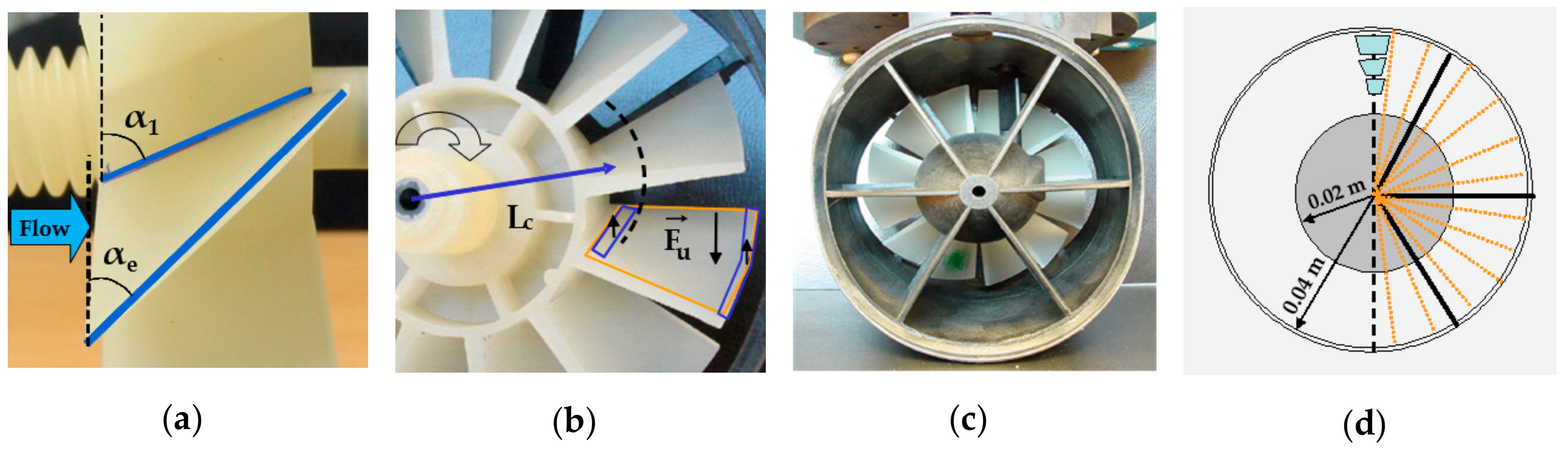
The final part of the study validated the numerical model results with measurements obtained empirically with a real instrument. Hence, it was necessary to geometrically characterize the turbine of the meter (Figure 5).

From the velocity profiles obtained with CFD techniques, numerical calculations estimated the measurement error in each case. During the differential study of flow forces, average cell velocities in each section of cut were assigned. To discern the velocities at each point of the pipe section, 15° cut lines starting from the pipe centre were extracted (Figure 5d).

Each cutting line (orange), with 19 velocity vectors, as well as the centre pivot and flow-straightening vanes (black), covered the entire section of the pipe (Figure 5c). Simulations were carried out with half of the pipe, reference case and gate valve, and 12 cut lines were extracted. In the case of the butterfly valve, 24 lines were extracted.

The behaviour of the meter in a pipe with a fully developed velocity profile was studied to extract a calibration function between the resistant moment and the rotational speed of the turbine, proportional to the circulating flow. This function was defined and associated to the variation in the rotor angular velocity with distorted profiles.

In order to assess the rotational speed of the turbine with distorted water flow, the water forces applied on the rotor blades were first recalculated. Then, iteratively, they were confronted with the resistant forces obtained from the previous function until they found the rotational speed of the turbine that matched the resistant torque with the driving torque produced by the distorted flow. The measurement error was estimated from the comparison between rotational speeds obtained with the distorted profile and fully developed profile.

2.4. Experimental Validation

The influence of water flow disturbances on the measurement error of a horizontal-axis turbine meter was investigated in the ITA Sustainable Urban Water Management test bench at the Universitat Politècnica de València, Valencia, Spain.

The principal elements used on the test bench included an electromagnetic flow meter with a precision of ±0.5%, a volumetric meter with a reading precision from ±0.5 to ±2%, a 0–16 bar range pressure transducer accurate to ±0.28%, Bourdon-type manometers of up to 1.6 MPa with a precision of ±0.5% on the full scale, two 18.5 kW pumps installed in parallel, epoxy-coated cast iron pipes of DN 80, a personal computer and a data acquisition system.

As recommended in standard [30], a laboratory test of Woltman meter performance was contrasted with more accurate measuring devices, such as an electromagnetic flowmeter and a precision volumetric meter, to obtain measurement errors. The results were presented graphically by means of the accuracy curve that represents the ratio of the measurement error versus actual flow rate range.

3. Results and Discussion

3.1. Theoretical Analysis

The main element of a horizontal-axis Woltman meter is the turbine on which the flow of water reaches the rotor in the axial direction. This speed at which the element rotates depends on the water velocity and the incidence on meter blades.

The volume circulated through the instrument is related to the number of turns of the turbine with a fully developed water flow.

Accurate measurement of water volume occurs with a balance between forces with a fully developed water flow. As in an engine, the driving torque (M_drive) is in equilibrium with the drag torque (M_drag) caused by the bearing, the hub disk friction, the tip clearance and the hub fluid drag [31]. When the velocity profile is altered, the driving torque acting on the turbine may differ from that obtained with the fully developed profile measuring the incorrect volume. In a steady-state regime, there is always a balance between forces; however, depending on the profile, this balance will be achieved at different rotational speeds of the turbine (Equation (1)).

$$M_{\mathit{drive} \mathit{axis} \mathit{turbine}}{=M}_{\mathit{drag}}$$

(1)

The measurement reliability of the Woltman meter is unknown when the driving torque of the incident water jet varies with distorted velocity profiles. In this case, the incidence of water flow on the turbine must be analysed (Figure 6).

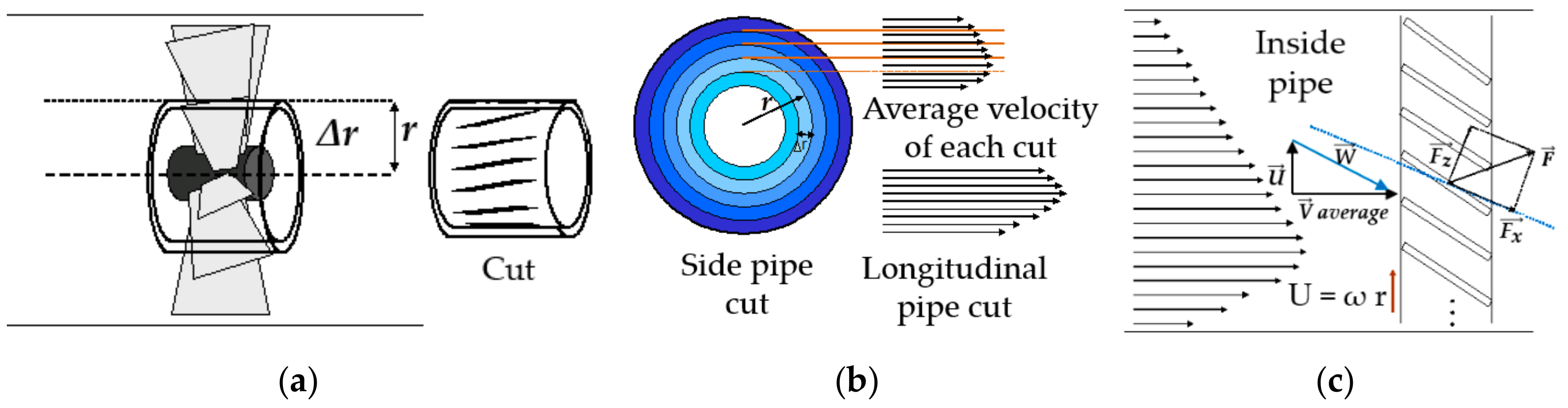
A differential study of the turbine was carried out, assuming a cylindrical control volume of radius r and thickness Δr with fluid moving through it (Figure 6a). When visualizing the turbine blades, the forces acting on this element in the entire section of the pipe can be considered. On each cylinder, there is a flow ring of thickness Δr and radius r, which represents the velocity vectors at the meter entrance. The velocity profiles that cover the entire entrance section of the meter are also broken down into concentric circles with an average velocity (Figure 6b).

In this way, in a steady-state regime, two forces acting on the turbine can be distinguished as a consequence of the incidence of water flow, the drag effort $\overrightarrow{F_x}$ in the same direction of the flow and the lift effort $\overrightarrow{F_z}$, perpendicular to it (Figure 6c).

These efforts are caused by the relative velocity of the fluid impacting on the blade $\overrightarrow{W}$, which depends both on the average axial velocity of the fluid $\overrightarrow{V}$ at the control volume and on the tangential velocity $\overrightarrow{U}$ of the moving turbine. The axial velocity is determined by the velocity profile that reaches the entrance section of the meter, while the tangential velocity, $\overrightarrow{U}$, and is proportional to the rotor angular velocity ω of the turbine. Angular velocity ω is a function of $\overrightarrow{V}$ and radius r (Equation (2)).

$$\overrightarrow{W}=\overrightarrow{V}-\overrightarrow{U},$$

(2)

where $\overrightarrow{U}=\omega r$ and $\overrightarrow{V}$ is the average velocity of the fluid in each differential element.

With knowledge of the geometry of the turbine and the velocities described above, it is possible to deduce the differential stresses exerted on the blade (Equations (3) and (4)).

$${\Delta F}_x=\frac{1}{2} \rho \Delta A W^2 C_x$$

(3)

$${\Delta F}_z=\frac{1}{2} \rho \Delta A W^2 C_z,$$

(4)

where ΔA is the area differential L_c Δr, ρ is the fluid density (kg m⁻³), W is the incident velocity and C_x and C_z are the drag and lift coefficients, respectively, depending on the angle of incidence of the turbine design and the kinematic viscosity of the fluid.

In this study, flat blades were considered for the cases studied because their geometric characteristics are difficult to adjust to any profile characterized. The C_z for flat blades is a function of its angle of incidence and can be approximated with the expression $C_z=2\pi \frac{\mathit{sen} i}{2}$ [32]. The drag coefficient is simplified to C_x ≈ 0, considering an ideal fluid (zero kinematic viscosity).

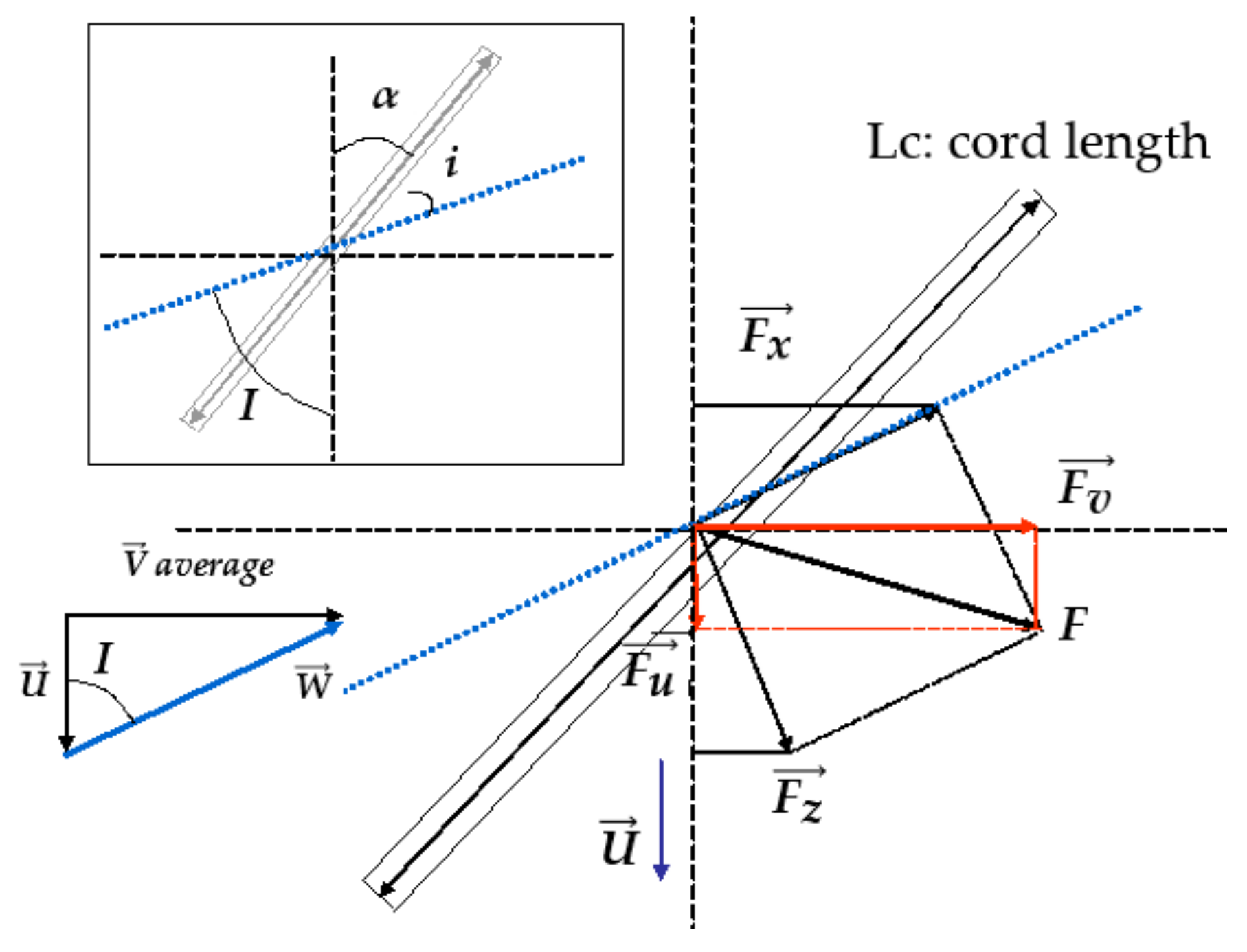
Thus, each fragment of the velocity profile will have an incident velocity and a variable angle i, formed between incident velocity $\overrightarrow{W}$ with the cord length of the blade Lc. In addition, the angle α will be the one that forms the blade with the vertical axis and will depend on the geometry of the blade that varies depending on the cutting radius. The angle I will be the sum of previous ones for each differential section (Figure 7).

Projecting resulting $\overrightarrow{F}$ in the flow direction and the turbine rotation is possible to obtain values of $\overrightarrow{F_v}$ and $\overrightarrow{F_u}$, corresponding to the axial force on the turbine and the motor force that generates a torque, respectively (Equations (5) and (6)).

$${\Delta F}_v=\frac{1}{2} \rho \Delta A W^2 \left(C_z\mathit{cos}\left(I\right){+ C}_x\mathit{sin}\left(I\right)\right)$$

(5)

$${\Delta F}_u=\frac{1}{2}{ \rho \Delta A W}^2 \left(C_z\mathit{sin}\left(I\right){+ C}_x\mathit{cos}\left(I\right)\right)$$

(6)

The drive torque for each differential cutting r transmitted to the turbine shaft by the effort ΔF_u, is calculated by Equation (7).

$${\Delta M}_{\mathit{blade}}=r {\Delta F}_u$$

(7)

The total driving torque generated by the water flow was obtained by adding all the motor forces extracted in each concentric fillet portion of velocity vectors by the number of turbine blades (Equations (8) and (9)).

$$M_{\mathit{drive} \mathit{axis} \mathit{turbine}}= {\displaystyle \sum }_{i=r}{\displaystyle \sum }_{z=\mathit{number} \mathit{of} \mathit{blades}}{\left({\Delta F}_u\right)}_z{ r}_i$$

(8)

$$M_{\mathit{drive} \mathit{axis} \mathit{turbine}}=\frac{1}{2}\iint {\rho L}_c{ W}^2\left(C_z\mathit{sin}\left(I\right) {- C}_x\mathit{cos}\left(I\right)\right) r dr$$

(9)

When the water flow is distorted by some type of hydraulic element, the driving torque on the turbine varies, causing a different angular velocity of the rotor than would occur with an undistorted flow. When the balance of forces is broken, and reached at a different rotation speed, measurement errors occur.

As mentioned, the driving torque for a distorted flow will differ from the drag-resistant torque of the instrument found by the equation ${(M}_{\mathit{drag}}{= a \omega }^2)$ for that flow. Comparing both torques, an approximate rotor angular velocity is estimated. The calculations will be repeated until rotational speed ω₀ matches the functions of drag torque and drive torque, and provides the new angular velocity of the turbine.

The rotor angular velocity (ω), estimated with the proposed methodology for distorted flow, can be compared with fully developed velocity profile results, estimating the error ($\epsilon$) produced by hydraulic elements upstream of the Woltman meter for the whole flow operating range of the device (Equation (10)).

$${\epsilon }_Q=\frac{{\omega }_{\mathit{distorted}} -{ \omega }_{\mathit{fully} \mathit{developed}}}{{\omega }_{\mathit{fully} \mathit{developed}}}$$

(10)

3.2. Computational Fluid Simulation

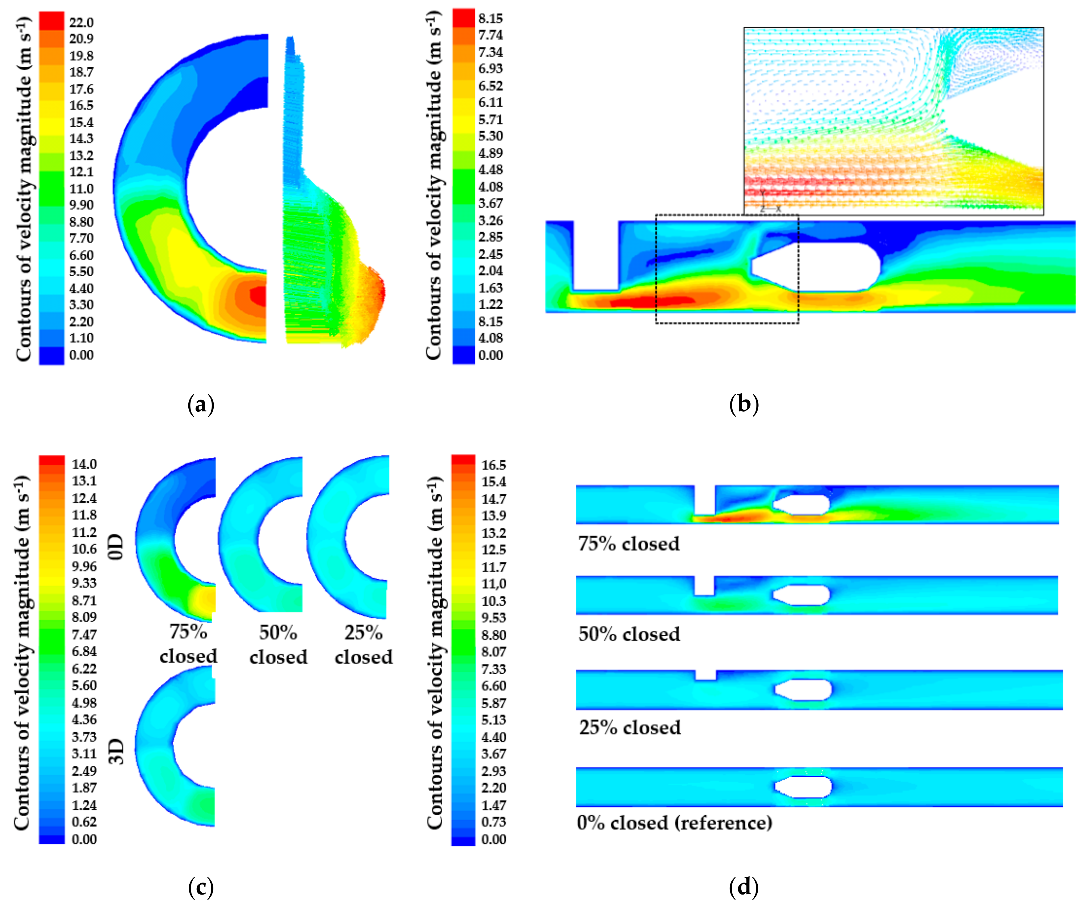
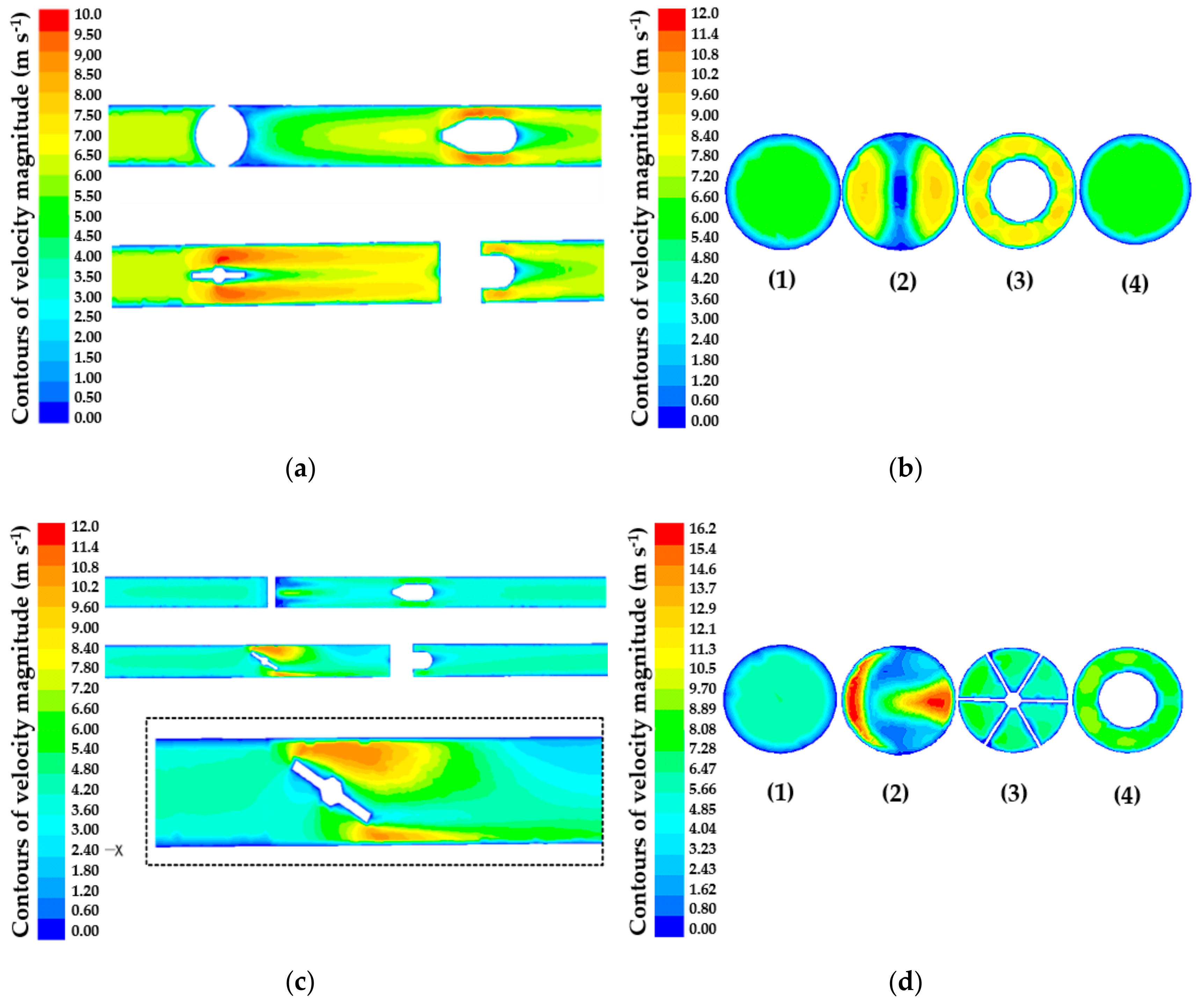
The velocity profiles distorted by a gate valve present different behaviours according to the simulated installation configuration (Figure 8).

The gate valve yields high-flow velocities in the lower part of the pipe when water flows through the gate, and creates lower-velocity turbulence zones in the upper part [33]. This behaviour can affect the measurement and varies with the distance to the Woltman meter.

In Figure 8a, the simulation results show that the velocity profiles in the turbine entrance section of the meter were very distorted, with very high velocities at the lower part of the pipe and more moderate at the top. In this case, the distance between the hydraulic element and the measuring instrument is too short and velocity profiles are unable to fully develop. The incident forces impacting on the turbine blades are asymmetric.

In Figure 8b, the distortions in the flow originated in the area near the gate valve. At this area, for a 34 m³ h⁻¹ flow rate corresponding an average flow velocity of 2 m s⁻¹, fluid velocities up to 8.15 m s⁻¹ are reached. Moreover, it is possible to observe reverse flows and swirls of water and even null velocity in the upper area of the pivot.

In Figure 8c, comparing the degree of closure of 75% in 0D and 3D, the flow behaviour is justified by a more regular flow due to the straight pipe distance between elements. However, this flow regularization is also conditioned by the degree of distortion caused. For example, for a degree of closure of 50% at 0D, average velocities in the lower area of the pivot are high (5 m s⁻¹–5.5 m s⁻¹), but lower than the velocities obtained with 75% closed at 3D (6 m s⁻¹–7 m s⁻¹).

In Figure 8d, the effect of closure is perceived. Small valve closure produces low flow distortions and the water velocity profile is stabilised upon reaching the meter.

According to the CFD simulations, the flow behaviour was influenced by a gate valve with different closures (0%, 50% and 75%) and distances (0D and 3D) to the meter. Increasing the degree of closure and the proximity of the meter, alters the velocity profile at the entrance of the instrument, causing the distortion of the flow and affecting the measurement accuracy [4]. This means that both parameters must be taken into account to evaluate the distortion of the flow that originates from each possible disturbing element and study the required straight distance until a full velocity profile is developed.

The butterfly valves consist of a circular plate with a section equal to the pipe used to control the flow. This disc has a vertical axis of rotation whereby the closing of the valve produces a change in the fluid flow direction by diverting velocity profiles towards paths perpendicular to this axis of rotation. When the valve is completely open, it reduces the section of water way, increasing the average water velocity in the pipe [34]. This behaviour may be confirmed in other studies that used CFD techniques to simulate distortion water flow with butterfly valves with different degrees of closure [35,36].

The simulated results with the butterfly valve open and 30° closed reflect a distortion of the fluid that differs from that caused by the gate valve (Figure 9).

In Figure 9a, the longitudinal pipe sections can be observed in two planes. In Figure 9b, velocity variations are seen to be quite homogeneous on both sides of the conduction. This flow effect produces a balanced incident flow at the meter entrance (position 3).

When the valve is 30° closed, there is no symmetrical distribution of the velocities. As can be seen, the flow perturbation in this case is very different from that caused by a gate valve. In Figure 9c, a slightly closed butterfly valve generates asymmetric flow disturbances in both parts of longitudinal sections.

Figure 9d shows the evolution of the velocity profile at different positions of measurement. Upstream of the measurement point (case 3), the magnitude of the velocities is quite homogeneous throughout the cross-section.

Studies show that CFD techniques can be used to evaluate the hydraulic behaviour of flow regulating valves. Research on butterfly valves under different opening range [26,37,38], and gate valves under different opening [4,39] or partial closing [33] conditions has been computational simulated under a wide range of flow conditions, using standard k-ε turbulent model with CFD solver software.

3.3. Numerical Analysis

The CFD-simulation results allowed the estimation of the relationship between the drag-resistant torque (M_drag) in N m and the rotational speed of the turbine (ω) in rad s⁻¹, proportional to the flow through the conduction (Q) in m³ h⁻¹ (Equations (11) and (12)). Then, $\omega$ can be used for the prediction of measurement error as follows:

$$M_{\mathit{drag} }= 0.00035 {\omega }^{1.99883} \left(R^2=1\right)$$

(11)

$$Q=1.399 \omega \left(R^2=1\right)$$

(12)

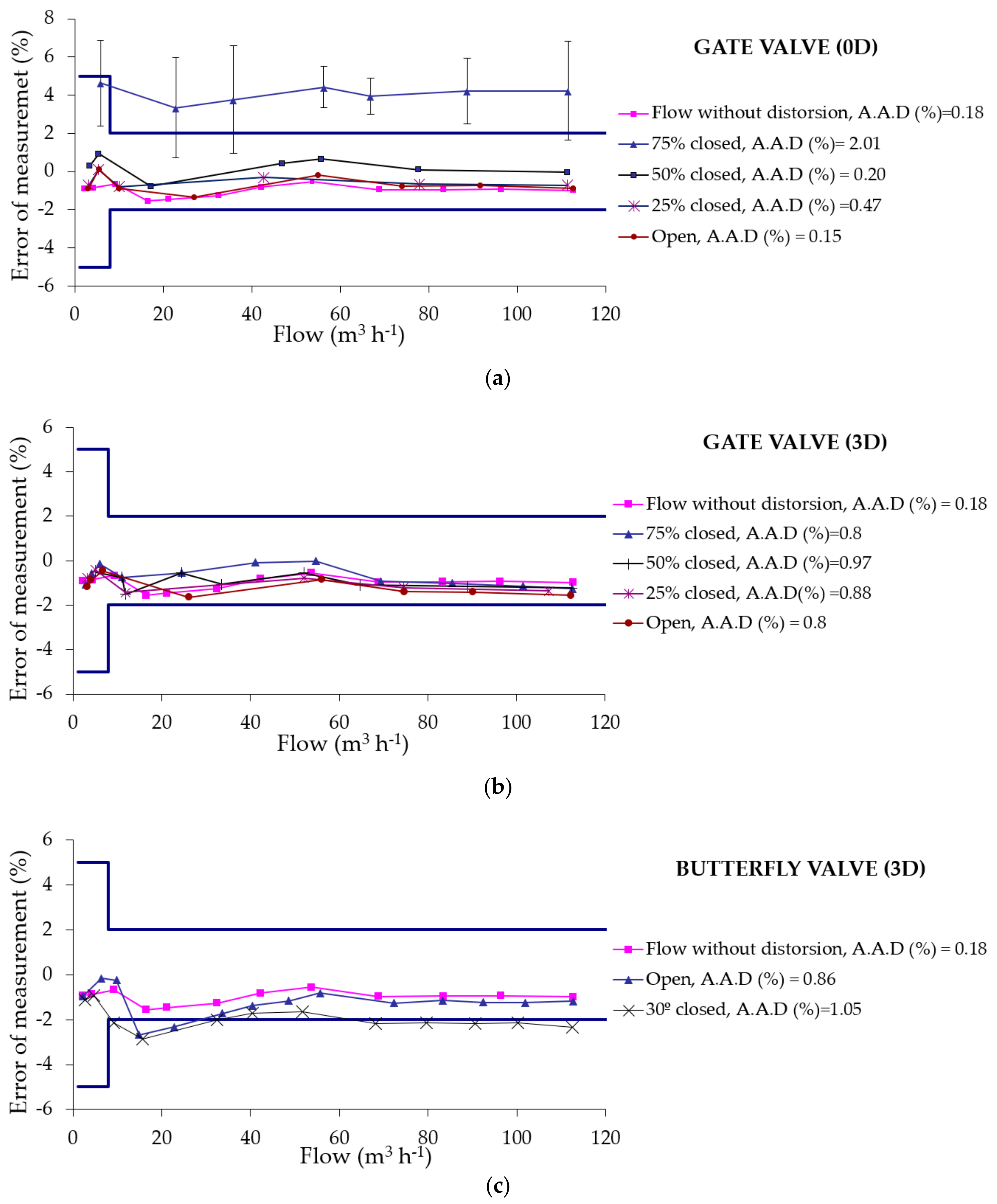
According to this approximation, the numerical errors ($\epsilon$) were obtained for each of the proposed cases. In the case of the gate valve (

Table 2. Relative errors caused by flow distortions generated by a 0D and 3D gate valve for 80 mm Woltman meter.

Degree Closure	Variable	Distance to Woltman Meter (0D)					Distance to Woltman Meter (3D)
75%	Flow (m3 h−1)	17.35	34.70	52.10	69.40	104.10	17.5	35.1	52.67	70.21	105.3
	ωdeveloped (rad s−1)	24.27	48.57	72.85	97.13	145.69	24.6	49.1	73.69	98.24	147.4
	ωdistorted (rad s−1)	34.55	69.86	105.45	141.01	212.20	25.1	50.4	75.03	100.6	149.9
	Error (%)	42.36	43.83	44.75	45.18	45.65	1.66	2.56	1.82	2.4	1.72
50%	Flow (m3 h−1)	17.27	34.55	51.83	69.11	103.66	-	-	-	-	-
	ωdeveloped (rad s−1)	24.17	48.34	72.52	96.69	145.04	-	-	-	-	-
	ωdistorted (rad s−1)	24.56	49.26	73.88	98.54	147.83	-	-	-	-	-
	Error (%)	1.63	1.90	1.87	1.91	1.92	-	-	-	-	-
25%	Flow (m3 h−1)	17.33	34.68	52.02	69.36	104.04	-	-	-	-	-
	ωdeveloped (rad s−1)	24.25	48.53	72.79	97.05	145.58	-	-	-	-	-
	ωdistorted (rad s−1)	24.05	48.15	72.21	96.25	144.40	-	-	-	-	-
	Error (%)	−0.82	−0.78	−0.80	−0.83	−0.81	-	-	-	-	-

D: pipe diameter; ω: turbine rotation speed.

), as the distortion caused is smaller, the measurement error is closer to the one that would occur under ideal flow conditions.

Table 2 shows that the extreme case, placing a 75% closed valve at 0D to the meter, can cause over-registration errors of approximately +45%. However, there is a significant reduction in measurement error simply by opening the valve and causing less distortion.

Thus, with a closure of 25% at 0D, the errors obtained are smaller, approximately −0.8%, for the entire range of operating flows. Moreover, in the case of 75% closed, the error decreases considerably from approximately +40% to +2% when the valve installation is placed with 3D straight pipe in between the meter.

The results for the butterfly valve analysis show that metering errors are similar and almost zero, since the flow is stabilized after 3D straight conduction (

Table 3. Relative errors caused by flow distortions generated by a 3D butterfly valve for 80 mm Woltman meter.

Variable	Open					Closed 30°
Flow (m3 h−1)	17.51	35.30	52.70	70.45	105.33	17.50	35.15	52.00	70.32	104.85
ωdeveloped (rad s−1)	24.60	49.08	73.50	98.10	147.38	24.55	49.30	73.80	98.45	147.80
ωdistorted (rad s−1)	24.40	48.90	73.05	97.70	146.85	24.30	49.10	73.50	98.20	147.15
Error (%)	−0.81	−0.37	−0.61	−0.41	−0.36	−1.02	−0.41	−0.41	−0.25	−0.44

D: pipe diameter; ω: turbine rotation speed.

).

3.4. Experimental Validation

In this study, experimental validation was conducted to assure the accuracy of the model. Figure 10 illustrates the results of laboratory tests for all study cases. Three measurements were taken for each flow rate, having in all cases an average absolute deviation (A.A.D) of the error under 2.01%. Only the 0D gate valve test with 75% closure showed more variability in the results (Figure 10a). Particularly, in this laboratory test the turbulence generated by the closed valve and the higher velocities justify this deviation. Average absolute deviation is estimated for each flow rate measurement in every test studied. No outliers were detected during the tests.

The experimental results obtained validate the numerical model proposed. Laboratory data are qualitatively similar to the numerical ones in most configurations. Only in the case of the 75% gate valve closed at 0D were the measurement errors extracted from the model (+40%) markedly higher than the experimental ones. In this case, the results can be justified since the design of the rotor blades and the simulation of the moving turbine were considered and an over estimation of rotational speed was achieved.

4. Conclusions

Even today, many flow measuring meters commonly used in water irrigation systems are inconveniently installed. In most cases, this is due to the lack of knowledge of the technical staff that is not familiar with or do not follow the manufacturer’s recommendations regarding installation or maintenance.

In this study, it was possible to propose a simplified numerical model capable of estimating the magnitude of the measurement errors caused by the installation of gate and butterfly valves close to a Woltman meter. The proposed method, validated by experimentation, demonstrates that fluid upstream obstacles can cause the velocity profile to distort and can influence meter performance.

Furthermore, the asymmetrical velocity profile entering through the Woltman meter resulted in higher measurement errors. In some cases, the water was forced to pass from the bottom or lateral section of the pipe, altering the rotor’s torque balance, thereby affecting meter accuracy.

Finally, this work showed the importance of adequate meter installation and how flow disturbance affect the registered measurement of the water consumed in irrigation areas. The proposed simplified model for error estimation can, effectively, reduce the high cost of experimental testing.

References

- Pardo, M.A.; Manzano, J.; Cabrera, E.; García-Serra, J. Energy audit of irrigation networks. Biosyst. Eng. 2013, 115, 89–101. [Google Scholar] [CrossRef] [Green Version]
- Zapata, N.; Salvador, R.; Cavero, J.; Lecina, S.; López, C.; Mantero, N.; Anadón, R.; Playán, E. Field test of an automatic controller for solid-set sprinkler irrigation. Irrig. Sci. 2013, 31, 1237–1249. [Google Scholar] [CrossRef] [Green Version]
- Arregui, F.; Cabrera, E., Jr.; Cobacho, R. Integrated Water Meter Management, 1st ed.; International Water Association: London, UK, 2007; ISBN 978-1-84339-034-3. [Google Scholar]
- Sapra, M.K.; Bajaj, M.; Kundu, S.N.; Sharma, B.S.V.G. Experimental and CFD investigation of 100 mm size cone flow elements. Flow Meas. Instrum. 2011, 22, 469–474. [Google Scholar] [CrossRef]
- Baker, R.C. Turbine and related flowmeters. In Flow Measurement Handbook: Industrial Designs, Operating Principles, Performance, and Applications; Cambridge University Press: Cambridge, UK, 2016; pp. 279–326. ISBN 978-1-107-05414-1. [Google Scholar]
- Lysak, P.D.; Jenkins, D.M.; Capone, D.E.; Brown, W.L. Analytical model of an ultrasonic cross-correlation flow meter, part 1: Stochastic modeling of turbulence. Flow Meas. Instrum. 2008, 19, 1–7. [Google Scholar] [CrossRef]
- Venugopal, A.; Agrawal, A.; Prabhu, S.V. Influence of blockage and upstream disturbances on the performance of a vortex flowmeter with a trapezoidal bluff body. Measurement 2010, 43, 603–616. [Google Scholar] [CrossRef]
- Singh, R.K.; Singh, S.N.; Seshadri, V. CFD prediction of the effects of the upstream elbow fittings on the performance of cone flowmeters. Flow Meas. Instrum. 2010, 21, 88–97. [Google Scholar] [CrossRef]
- Piechota, P.; Synowiec, P.; Andruszkiewicz, A.; Wędrychowicz, W. Selection of the relevant turbulence model in a CFD simulation of a flow disturbed by hydraulic elbow — comparative analysis of the simulation with measurements results obtained by the ultrasonic flowmeter. J. Therm. Sci. 2018, 27, 413–420. [Google Scholar] [CrossRef]
- Zhuang, Y.; Zhang, N.; Ma, L.; Huang, Y. Numerical investigation of liquid flowmeter calibration device based on CFD. J. Phys. Conf. Ser. 2018, 1074, 1–7. [Google Scholar] [CrossRef]
- Liu, W.; Xu, Y.; Zhang, T.; Qi, F. Experimental optimization for dual support structures cone flow meters based on cone wake flow field characteristics. Sens. Actuator A Phys. 2015, 232, 115–131. [Google Scholar] [CrossRef]
- Blocken, B.; Gualtieri, C. Ten iterative steps for model development and evaluation applied to Computational Fluid Dynamics for environmental fluid mechanics. Environ. Model. Softw. 2012, 33, 1–22. [Google Scholar] [CrossRef]
- Bonakdari, H.; Zinatizadeh, A.A. Influence of position and type of Doppler flow meters on flow-rate measurement in sewers using computational fluid dynamic. Flow Meas. Instrum. 2011, 22, 225–234. [Google Scholar] [CrossRef]
- Singh, R.K.; Singh, S.N.; Seshadri, V. Study on the effect of vertex angle and upstream swirl on the performance characteristics of cone flowmeter using CFD. Flow Meas. Instrum. 2009, 20, 69–74. [Google Scholar] [CrossRef]
- Tang, P.; Juárez, J.M.; Li, H. Investigation on the effect of structural parameters on cavitation characteristics for the Venturi tube using the CFD method. Water 2019, 11, 2194. [Google Scholar] [CrossRef] [Green Version]
- Zheng, D.; Zhang, P.; Xu, T. Study of acoustic transducer protrusion and recess effects on ultrasonic flowmeter measurement by numerical simulation. Flow Meas. Instrum. 2011, 22, 488–493. [Google Scholar] [CrossRef]
- Qin, L.; Hu, L.; Mao, K.; Chen, W.; Fu, X. Flow profile identification with multipath transducers. Flow Meas. Instrum. 2016, 52, 148–156. [Google Scholar] [CrossRef]
- Palau, C.V.; do Bomfim, G.V.; de Azevedo, B.M.; Peralta, I.B. Numerical study of upstream disturbances on the performance of electromagnetic and ultrasonic flowmeters. Sci. Agric. (Piracicaba, Braz.) 2019, 77, 1–8. [Google Scholar] [CrossRef]
- Ribeiro, A.S.; Loureiro, D.; Martins, L.; Sousa, J.A.; Batista, E.; Dias, L.; Soares, A.C. Measurement uncertainty of turbine flow meter calibration used in conformity assessment for water management. J. Phys. Conf. Ser. 2018, 1065, 092006. [Google Scholar] [CrossRef]
- Simão, M.; Besharat, M.; Carravetta, A.; Ramos, H.M. Flow velocity distribution towards flowmeter accuracy: CFD, UDV, and field tests. Water 2018, 10, 1807. [Google Scholar] [CrossRef] [Green Version]
- Moosa, M.; Hekmat, M.H. Numerical investigation of turbulence characteristics and upstream disturbance of flow through standard and multi-hole orifice flowmeters. Flow Meas. Instrum. 2019, 65, 203–218. [Google Scholar] [CrossRef]
- Borkar, K.; Venugopal, A.; Prabhu, S.V. Pressure measurement technique and installation effects on the performance of wafer cone design. Flow Meas. Instrum. 2013, 30, 52–59. [Google Scholar] [CrossRef]
- Weissenbrunner, A.; Fiebach, A.; Schmelter, S.; Bär, M.; Thamsen, P.U.; Lederer, T. Simulation-based determination of systematic errors of flow meters due to uncertain inflow conditions. Flow Meas. Instrum. 2016, 52, 25–39. [Google Scholar] [CrossRef] [Green Version]
- Liu, Q.; Ye, J.; Zhang, G.; Lin, Z.; Xu, H.; Jin, H.; Zhu, Z. Study on the metrological performance of a swirlmeter affected by flow regulation with a sleeve valve. Flow Meas. Instrum. 2019, 67, 83–94. [Google Scholar] [CrossRef]
- Zhen, W.; Tao, Z. Computational study of the tangential type turbine flowmeter. Flow Meas. Instrum. 2008, 19, 233–239. [Google Scholar] [CrossRef]
- Mu, Y.; Liu, M.; Ma, Z. Research on the measuring characteristics of a new design butterfly valve flowmeter. Flow Meas. Instrum. 2019, 70, 101651. [Google Scholar] [CrossRef]
- Mignot, E.; Bonakdari, H.; Knothe, P.; Lipeme Kouyi, G.; Bessette, A.; Rivière, N.; Bertrand-Krajewski, J.-L. Experiments and 3D simulations of flow structures in junctions and their influence on location of flowmeters. Water Sci. Technol. 2012, 66, 1325–1332. [Google Scholar] [CrossRef]
- Saboohi, Z.; Sorkhkhah, S.; Shakeri, H. Developing a model for prediction of helical turbine flowmeter performance using CFD. Flow Meas. Instrum. 2015, 42, 47–57. [Google Scholar] [CrossRef]
- Versteeg, H.K.; Malalasekera, W. An Introduction to Computational Fluid Dynamics: The Finite Volume Method, 2nd ed.; Pearson Education Ltd: Harlow, UK, 2007; ISBN 978-0-13-127498-3. [Google Scholar]
- ISO 4064-2. Water Meters for Cold Potable Water and Hot Water—Part 2: Test Methods; ISO: Geneva, Switzerland, 2014. [Google Scholar]
- Tsukamoto, H.; Hutton, S.P. Theoretical prediction of meter factor for a helical turbine flowmeter. In Proceedings of the Conference on Fluid Control and Measurement, Tokyo, Japan, 2–5 September 1985. [Google Scholar]
- Wallis, R.A. Axial Flow Fans; Academic Press: New York, NY, USA, 1961; ISBN 978-1-4832-2784-9. [Google Scholar]
- Augusto, P.E.D.; Cristianini, M. Using Computational Fluid Dynamics (CFD) for evaluation of fluid flow through a gate valve. Int. J. Food Eng. 2012, 8, 1–11. [Google Scholar] [CrossRef]
- Corbera, S.; Olazagoitia, J.L.; Lozano, J.A. Multi-objective global optimization of a butterfly valve using genetic algorithms. ISA Trans. 2016, 63, 401–412. [Google Scholar] [CrossRef]
- Azad, A.; Baranwal, D.; Arya, R.; Diwakar, N. Flow analysis of butterfly valve using CFD. Int. J. Mod. Eng. Res. Technol. 2014, 4, 50–56. [Google Scholar]
- Dawy, A.; Sharara, A.; Hassan, A. A numerical investigation of the incompressible flow through a butterfly valve using CFD. Int. J. Emerg. Technol. Adv. Eng. 2013, 3, 1–7. [Google Scholar]
- Toro, A.D.; Johnson, M.C.; Spall, R.E. Computational fluid dynamics investigation of butterfly valve performance factors. J. Am. Water Works Assoc. 2015, 107, E243–E254. [Google Scholar] [CrossRef]
- Li, S.; Zhu, L.; Wang, W.; Xiao, K.; Xu, X.; Zhang, B. Analysis of Thermal-Fluid-Structure Coupling and Resonance Forecast for Link Butterfly Valve Under Small Opening. J. Shanghai Jiaotong Univ. (Sci.) 2019, 24, 341–350. [Google Scholar] [CrossRef]
- Lin, Z.; Ma, G.; Cui, B.; Li, Y.; Zhu, Z.; Tong, N. Influence of flashboard location on flow resistance properties and internal features of gate valve under the variable condition. J. Nat. Gas Sci. Eng. 2016, 33, 108–117. [Google Scholar] [CrossRef]
Figure 1.
Schematic configuration with meter and butterfly and air valve installed upstream the flow (a); horizontal-axis Woltman meter installed to register water consumption in an irrigation plot (b).
Figure 2.
Computational domain for gate valve simulations (a) and for butterfly valve simulations (b). In which, 0D or 3D indicates a distance of zero or 3 diameters to the meter, D stands for the diameter of the meter (80 mm).
Figure 3.
Cross-section and longitudinal views of Woltman meter (a); detail of the internal part of the horizontal-axis Woltman meter with the meter pivot and six flow-straightening vanes (b).
Figure 4.
Longitudinal detail of the grid used in simulations with the gate valve and fixed internal parts of the water meter (a); grid cross-sections at different positions of Computational Fluid Dynamics (CFD) domain (b). Positions: (1): entrance CFD domain; (2): 75% closed gate valve; (3): entrance meter pivot area.
Figure 5.
Side view (a) and front view (b) of the turbine and cut lines extracted from the inlet section to the blades (c,d) of the horizontal-axis Woltman meter. The turbine has 12 blades, six flow-straightening vanes, a 0.02 m radius of the pivot, a 0.038 m radius of the blade, 67° of αi and 47° of αe (torsion angles), a string length (Lc) of 0.12r + 0.022 and a volume-turn ratio of 1 rev: 1.24732 L.
Figure 6.
Cutting lines extracted from the horizontal-shaft-axis Woltman meter input section: cylindrical turbine section (a); cross-section of the pipe (b); longitudinal section of the inside of the pipe (c).
Figure 7.
Force analysis in a Woltman meter blade.
Figure 8.
Profile of velocities in the pipe section distorted by a gate valve near the horizontal-axis Woltman meter: cross-section (a) and longitudinal (b) upstream with 75% closure at 0D; cross-sections upstream at different distances and degrees of closure (c); longitudinal sections upstream at 0D for different degrees of closure (d). D: pipe diameter. In the cross and longitudinal pipe sections flow rate was approximately between 34 and 100 m3 h−1.
Figure 9.
Profile of velocities obtained by CFD simulations in the pipe distorted by a butterfly valve installed at a 3D pipe of the horizontal-axis Woltman meter: longitudinal section upstream for open valve (a); cross-section in different positions for open valve (b); longitudinal section of simulation for 30° closed valve (c); cross-sections in various positions for 30° closed valve (d). Positions: (1): upstream of the valve; (2): downstream of the valve; (3): meter pivot area; (4): downstream the meter.
Figure 10.
Measurement errors of the horizontal-axis Woltman meter caused by a gate valve with different closures at 0D (a) and 3D (b), and by an open and 30° closed butterfly valve to 3D (c). Average absolute deviation (A.A.D) of the error of measurement (%) for each flow rate. D: pipe diameter.