Modeling Groundwater Potential Zone in a Semi-Arid Region of Aseer Using Fuzzy-AHP and Geoinformation Techniques

 , , ,
, , , 
Abstract
:1. Introduction
- (a)
- propose a methodology for the identification and delineation of groundwater potential zones in Itwad-Khamis watershed using integrated techniques of RS, GIS with Fuzzy-AHP and demonstrate this by a case study;
- (b)
- carry out a sensitivity analysis and recognize the most sensitive factors that influence the identification of potential groundwater zones;
- (c)
- demonstrate geoinformation technology capabilities in groundwater mapping.
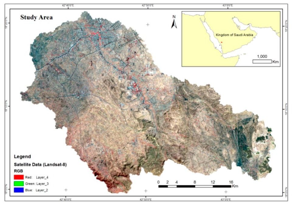
2. Study Area
3. Data Used and Methodology
3.1. Data and Material Used
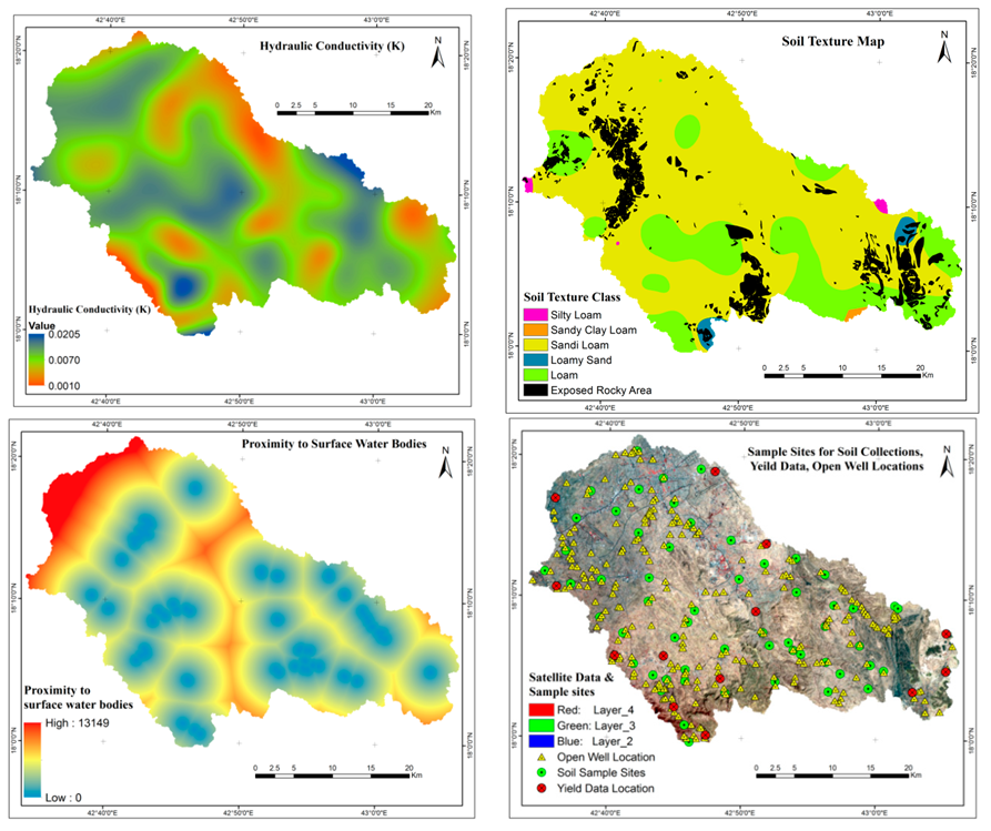
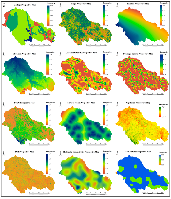
3.2. Spatial Data Processing for Groundwater Potential Zone Mapping
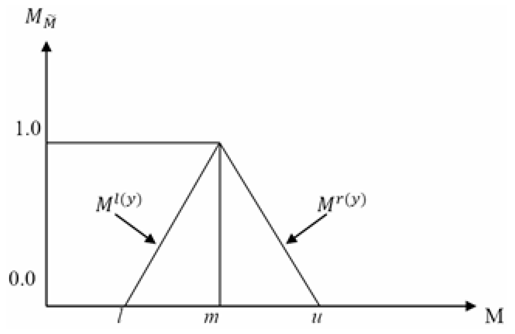
3.3. MCDM: Fuzzy Set Theory
3.4. Fuzzy Membership Function (FMF)
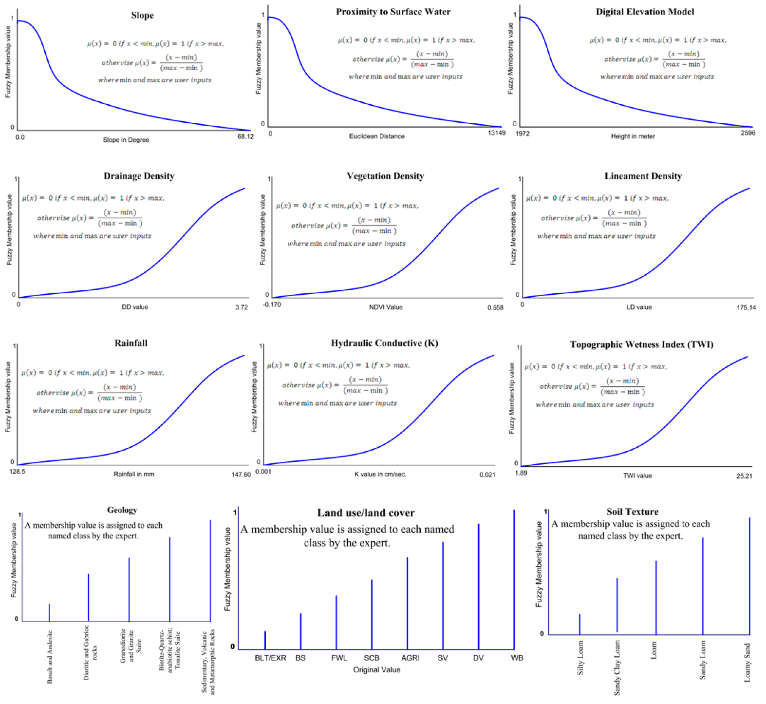
3.5. Feature Data Standardization Using FMFs
3.6. Weights Assignments and Normalization
3.7. Groundwater Potential Map Development
3.8. Sensitivity Analysis
3.9. Relative Operating Characteristics (ROC)
4. Results and Discussion
4.1. Weights Normalization for Thematic Maps
4.2. Validation of the Results
4.2.1. Sensitivity Analysis
4.2.2. Overlay Method
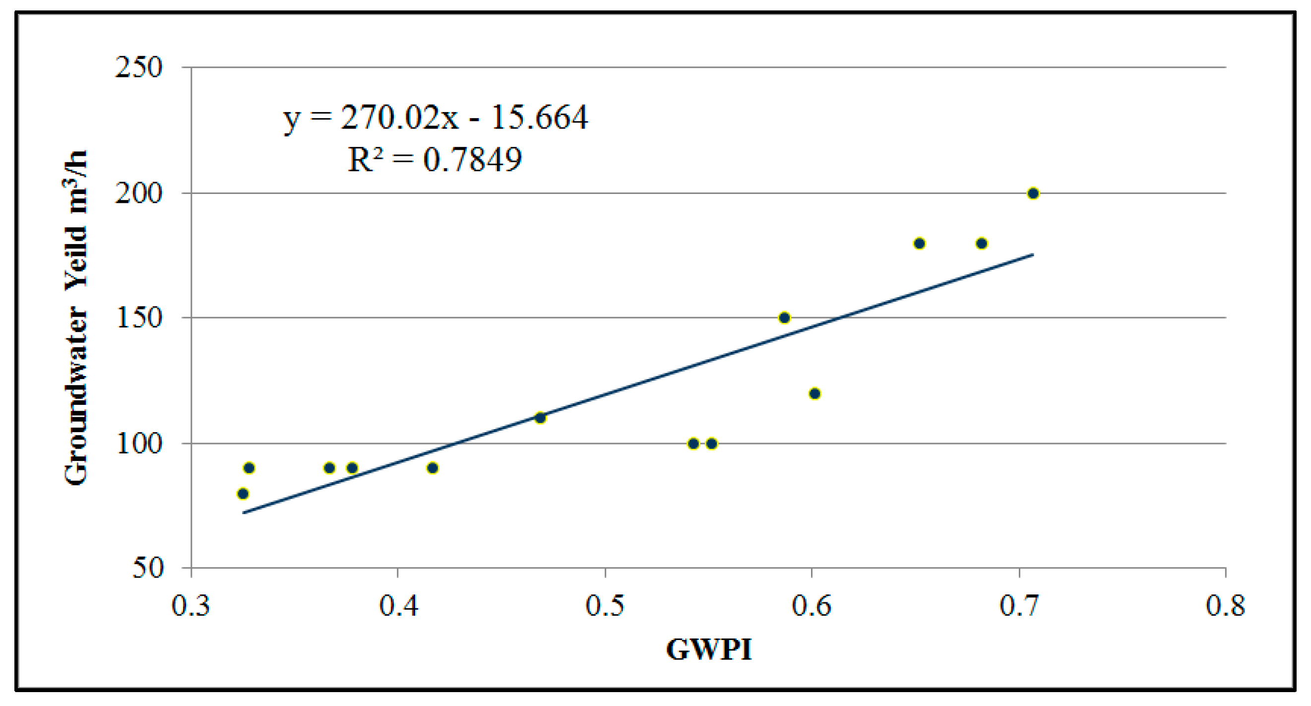
4.2.3. Relative Operating Characteristics (ROC)
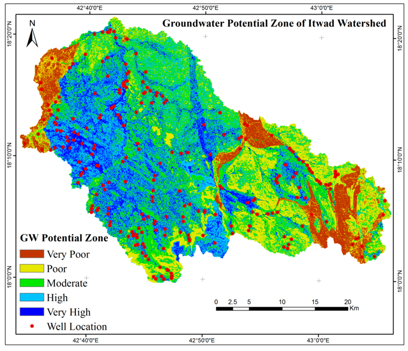
4.3. Analysis of GWPZ Classification Map
5. Conclusions
Supplementary Materials
Author Contributions
Funding
Acknowledgments
Conflicts of Interest
References
- Naghibi, S.A.; Pourghasemi, H.R.; Pourtaghi, Z.S.; Rezaei, A. Groundwater Qanat Potential Mapping Using Frequency Ratio and Shannon’s Entropy Models in the Moghan Watershed, Iran. Earth Sci. Inform. 2015. [Google Scholar] [CrossRef]
- IPCC. Climate Change: The Scientific Basis. Contribution of Working Group I to the Third Assessment Report of the Intergovernmental Panel on Climate Change; Houghton, J.T., Ding, Y., Griggs, D.J., Noguer, M., van der Linden, P.J., Dai, X., Maskell, K., Johnson, C.A., Eds.; Cambridge University Press: Cambridge, UK, 2001. [Google Scholar]
- Senanayake, I.P.; Dissanayake, D.M.D.O.K.; Mayadunna, B.B.; Weerasekera, W.L. An Approach to Delineate Groundwater Recharge Potential Sites in Ambalantota, Sri Lanka Using GIS Techniques. Geosci. Front. 2016. [Google Scholar] [CrossRef] [Green Version]
- Manap, M.A.; Nampak, H.; Pradhan, B.; Lee, S.; Sulaiman, W.N.A.; Ramli, M.F. Application of Probabilistic-Based Frequency Ratio Model in Groundwater Potential Mapping Using Remote Sensing Data and GIS. Arab. J. Geosci. 2014. [Google Scholar] [CrossRef]
- Das, S.; Pardeshi, S.D. Morphometric Analysis of Vaitarna and Ulhas River Basins, Maharashtra, India: Using Geospatial Techniques. Appl. Water Sci. 2018. [Google Scholar] [CrossRef] [Green Version]
- Pathak, D. Delineation of groundwater potential zone in the Indo-Gangetic plain through GIS analysis. J. Inst. Sci. Technol. 2017. [Google Scholar] [CrossRef]
- Almazroui, M. Sensitivity of a Regional Climate Model on the Simulation of High Intensity Rainfall Events over the Arabian Peninsula and around Jeddah (Saudi Arabia). Theor. Appl. Climatol. 2011. [Google Scholar] [CrossRef] [Green Version]
- Vincent, P. Saudi Arabia: An Environmental Overview; CRC Press: Boca Raton, FL, USA, 2008. [Google Scholar] [CrossRef]
- Abdullah, M.A.; Al-Mazroui, M.A. Climatological Study of the Southwestern Region of Saudi Arabia. I. Rainfall Analysis. Clim. Res. 1998, 9, 213–223. [Google Scholar] [CrossRef]
- Al-Jerash, M.A. Data for Climatic Water Balance in Saudi Arabia: 1970–1986 A.D.; Scientific Publishing Centre, King Abdulaziz University: Jeddah, Saudi Arabia, 1989; p. 144. [Google Scholar]
- Samad, N.A.; Bruno, V.L. The urgency of preserving water resources. Environ. News 2013, 21, 3–6. [Google Scholar]
- DeNicola, E.; Aburizaiza, O.S.; Siddique, A.; Khwaja, H.; Carpenter, D.O. Climate Change and Water Scarcity: The Case of Saudi Arabia. Ann. Glob. Health 2015. [Google Scholar] [CrossRef]
- Fetter, C.W. Applied Hydrogeology, 4th ed.; Prentice Hall: Englewood Cliffs, NJ, USA, 1994; pp. 543–591. [Google Scholar]
- Das, S. Comparison among Influencing Factor, Frequency Ratio, and Analytical Hierarchy Process Techniques for Groundwater Potential Zonation in Vaitarna Basin, Maharashtra, India. Groundw. Sustain. Dev. 2019. [Google Scholar] [CrossRef]
- Oh, H.J.; Kim, Y.S.; Choi, J.K.; Park, E.; Lee, S. GIS Mapping of Regional Probabilistic Groundwater Potential in the Area of Pohang City, Korea. J. Hydrol. 2011. [Google Scholar] [CrossRef]
- Mallick, J.; Al-Wadi, H.; Rahman, A.; Ahmed, M. Landscape Dynamic Characteristics Using Satellite Data for a Mountainous Watershed of Abha, Kingdom of Saudi Arabia. Environ. Earth Sci. 2014. [Google Scholar] [CrossRef]
- Silwal, C.B.; Pathak, D. Review on Practices and State of the Art Methods on Delineation of Ground Water Potential Using GIS and Remote Sensing. Bull. Dep. Geol. 2018. [Google Scholar] [CrossRef] [Green Version]
- Jha, M.K.; Chowdhury, A.; Chowdary, V.M.; Peiffer, S. Groundwater Management and Development by Integrated Remote Sensing and Geographic Information Systems: Prospects and Constraints. Water Resour. Manag. 2007. [Google Scholar] [CrossRef]
- Solomon, S.; Quiel, F. Groundwater Study Using Remote Sensing and Geographic Information Systems (GIS) in the Central Highlands of Eritrea. Hydrogeol. J. 2006. [Google Scholar] [CrossRef] [Green Version]
- Ganapuram, S.; Kumar, G.T.V.; Krishna, I.V.M.; Kahya, E.; Demirel, M.C. Mapping of Groundwater Potential Zones in the Musi Basin Using Remote Sensing Data and GIS. Adv. Eng. Softw. 2009. [Google Scholar] [CrossRef]
- Saha, D.; Dhar, Y.R.; Vittala, S.S. Delineation of Groundwater Development Potential Zones in Parts of Marginal Ganga Alluvial Plain in South Bihar, Eastern India. Environ. Monit. Assess. 2010. [Google Scholar] [CrossRef]
- Al-Adamat, R.A.N.; Foster, I.D.L.; Baban, S.M.J. Groundwater Vulnerability and Risk Mapping for the Basaltic Aquifer of the Azraq Basin of Jordan Using GIS, Remote Sensing and DRASTIC. Appl. Geogr. 2003. [Google Scholar] [CrossRef]
- Dar, I.A.; Sankar, K.; Dar, M.A. Remote Sensing Technology and Geographic Information System Modeling: An Integrated Approach towards the Mapping of Groundwater Potential Zones in Hardrock Terrain, Mamundiyar Basin. J. Hydrol. 2010. [Google Scholar] [CrossRef]
- Murthy, K.S.R. Ground Water Potential in a Semi-Arid Region of Andhra Pradesh—A Geographical Information System Approach. Int. J. Remote Sens. 2000. [Google Scholar] [CrossRef]
- Leblanc, M.; Favreau, G.; Tweed, S.; Leduc, C.; Razack, M.; Mofor, L. Remote Sensing for Groundwater Modelling in Large Semiarid Areas: Lake Chad Basin, Africa. Hydrogeol. J. 2007. [Google Scholar] [CrossRef]
- Abdalla, F. Mapping of Groundwater Prospective Zones Using Remote Sensing and GIS Techniques: A Case Study from the Central Eastern Desert, Egypt. J. Afr. Earth Sci. 2012. [Google Scholar] [CrossRef]
- Al-Abadi, A.; Al-Shamma, A. Groundwater Potential Mapping of the Major Aquifer in Northeastern Missan Governorate, South of Iraq by Using Analytical Hierarchy Process and GIS. J. Environ. Earth Sci. 2014, 10, 125–149. [Google Scholar]
- Rahmati, O.; Nazari Samani, A.; Mahdavi, M.; Pourghasemi, H.R.; Zeinivand, H. Groundwater Potential Mapping at Kurdistan Region of Iran Using Analytic Hierarchy Process and GIS. Arab. J. Geosci. 2015. [Google Scholar] [CrossRef]
- Joubert, A.; Stewart, T.J.; Eberhard, R. Evaluation of Water Supply Augmentation and Water Demand Management Options for the City of Cape Town. J. Multi Criteria Decis. Anal. 2003. [Google Scholar] [CrossRef]
- Machiwal, D.; Jha, M.K.; Mal, B.C. Assessment of Groundwater Potential in a Semi-Arid Region of India Using Remote Sensing, GIS and MCDM Techniques. Water Resour. Manag. 2011. [Google Scholar] [CrossRef]
- Pourghasemi, H.R.; Mohammady, M.; Pradhan, B. Landslide Susceptibility Mapping Using Index of Entropy and Conditional Probability Models in GIS: Safarood Basin, Iran. Catena 2012. [Google Scholar] [CrossRef]
- Chandio, I.A.; Matori, A.N.B.; WanYusof, K.B.; Talpur, M.A.H.; Balogun, A.L.; Lawal, D.U. GIS-Based Analytic Hierarchy Process as a Multicriteria Decision Analysis Instrument: A Review. Arab. J. Geosci. 2013. [Google Scholar] [CrossRef]
- Althuwaynee, O.F.; Pradhan, B.; Park, H.J.; Lee, J.H. A Novel Ensemble Bivariate Statistical Evidential Belief Function with Knowledge-Based Analytical Hierarchy Process and Multivariate Statistical Logistic Regression for Landslide Susceptibility Mapping. Catena 2014. [Google Scholar] [CrossRef]
- Singh, L.K.; Jha, M.K.; Chowdary, V.M. Multi-Criteria Analysis and GIS Modeling for Identifying Prospective Water Harvesting and Artificial Recharge Sites for Sustainable Water Supply. J. Clean. Prod. 2017. [Google Scholar] [CrossRef]
- Chowdhury, A.; Jha, M.K.; Chowdary, V.M. Delineation of Groundwater Recharge Zones and Identification of Artificial Recharge Sites in West Medinipur District, West Bengal, Using RS, GIS and MCDM Techniques. Environ. Earth Sci. 2010. [Google Scholar] [CrossRef]
- Hajkowicz, S.; Collins, K. A Review of Multiple Criteria Analysis for Water Resource Planning and Management. Water Resour. Manag. 2007. [Google Scholar] [CrossRef]
- Murthy, K.S.R.; Mamo, A.G. Multi-Criteria Decision Evaluation in Groundwater Zones Identification in Moyale-Teltele Subbasin, South Ethiopia. Int. J. Remote Sens. 2009. [Google Scholar] [CrossRef]
- Kaliraj, S.; Chandrasekar, N.; Magesh, N.S. Identification of Potential Groundwater Recharge Zones in Vaigai Upper Basin, Tamil Nadu, Using GIS-Based Analytical Hierarchical Process (AHP) Technique. Arab. J. Geosci. 2014. [Google Scholar] [CrossRef]
- Ouma, Y.O.; Tateishi, R. Urban Flood Vulnerability and Risk Mapping Using Integrated Multi-Parametric AHP and GIS: Methodological Overview and Case Study Assessment. Water 2014, 6, 1515–1545. [Google Scholar] [CrossRef]
- Rahaman, S.A.; Ajeez, S.A.; Aruchamy, S.; Jegankumar, R. Prioritization of Sub Watershed Based on Morphometric Characteristics Using Fuzzy Analytical Hierarchy Process and Geographical Information System—A Study of Kallar Watershed, Tamil Nadu. Aquat. Procedia 2015. [Google Scholar] [CrossRef]
- Mallick, J.; Singh, C.K.; Al-Wadi, H.; Ahmed, M.; Rahman, A.; Shashtri, S.; Mukherjee, S. Geospatial and Geostatistical Approach for Groundwater Potential Zone Delineation. Hydrol. Process. 2015. [Google Scholar] [CrossRef]
- Chen, V.Y.C.; Lien, H.P.; Liu, C.H.; Liou, J.J.H.; Tzeng, G.H.; Yang, L.S. Fuzzy MCDM Approach for Selecting the Best Environment-Watershed Plan. Appl. Soft Comput. J. 2011. [Google Scholar] [CrossRef]
- Kayastha, P.; Dhital, M.R.; De Smedt, F. Application of the Analytical Hierarchy Process (AHP) for Landslide Susceptibility Mapping: A Case Study from the Tinau Watershed, West Nepal. Comput. Geosci. 2013. [Google Scholar] [CrossRef]
- Millet, I.; Saaty, T.L. On the Relativity of Relative Measures—Accommodating Both Rank Preservation and Rank Reversals in the AHP. Eur. J. Oper. Res. 2000. [Google Scholar] [CrossRef]
- Hsieh, T.Y.; Lu, S.T.; Tzeng, G.H. Fuzzy MCDM Approach for Planning and Design Tenders Selection in Public Office Buildings. Int. J. Proj. Manag. 2004. [Google Scholar] [CrossRef]
- Altrock, C.V.; Krause, B. Multi-Criteria Decision Making in German Automotive Industry Using Fuzzy Logic. Fuzzy Sets Syst. 1994. [Google Scholar] [CrossRef]
- Opricovic, S.; Tzeng, G.H. Defuzzification within a Multicriteria Decision Model. Int. J. Uncertain. Fuzziness Knowl. Based Syst. 2003. [Google Scholar] [CrossRef]
- Li, S.P.; Will, B.F. A Fuzzy Logic System for Visual Evaluation. Environ. Plan. B 2005. [Google Scholar] [CrossRef] [Green Version]
- Wang, W.-D.; Xie, C.-M.; Du, X.-G. Landslides Susceptibility Mapping in Guizhou Province Based on Fuzzy Theory. Min. Sci. Technol. 2009, 19, 399–404. [Google Scholar] [CrossRef]
- Gorsevski, P.V.; Jankowski, P. An Optimized Solution of Multi-Criteria Evaluation Analysis of Landslide Susceptibility Using Fuzzy Sets and Kalman Filter. Comput. Geosci. 2010. [Google Scholar] [CrossRef]
- Al-Ruzouq, R.; Shanableh, A.; Yilmaz, A.G.; Idris, A.; Mukherjee, S.; Khalil, M.A.; Gibril, M.B.A. Dam Site Suitability Mapping and Analysis Using an Integrated GIS and Machine Learning Approach. Water 2019, 11, 1880. [Google Scholar] [CrossRef] [Green Version]
- Patra, S.; Mishra, P.; Mahapatra, S.C. Delineation of Groundwater Potential Zone for Sustainable Development: A Case Study from Ganga Alluvial Plain Covering Hooghly District of India Using Remote Sensing, Geographic Information System and Analytic Hierarchy Process. J. Clean. Prod. 2018. [Google Scholar] [CrossRef]
- Arulbalaji, P.; Padmalal, D.; Sreelash, K. GIS and AHP Techniques Based Delineation of Groundwater Potential Zones: A case study from Southern Western Ghats, India. Sci. Rep. 2019, 9, 2082. [Google Scholar] [CrossRef]
- Shahabi, H.; Hashim, M. Landslide susceptibility mapping using GIS-based statistical models and Remote sensing data in tropical environment. Sci. Rep. 2015, 5, 9899. [Google Scholar] [CrossRef] [Green Version]
- Adeyeye, O.A.; Ikpokonte, E.A.; Arabi, S.A. GIS-Based Groundwater Potential Mapping within Dengi Area, North Central Nigeria. Egypt. J. Remote Sens. Space Sci. 2018. [Google Scholar] [CrossRef]
- Pinto, D.; Shrestha, S.; Babel, M.S.; Ninsawat, S. Delineation of groundwater potential zones in the Comoro watershed, Timor Leste using GIS, remote sensing and analytic hierarchy process (AHP) technique. Appl. Water Sci. 2017, 7, 503–519. [Google Scholar] [CrossRef] [Green Version]
- Jasrotia, A.S.; Kumar, A.; Singh, R. Integrated Remote Sensing and GIS Approach for Delineation of Groundwater Potential Zones Using Aquifer Parameters in Devak and Rui Watershed of Jammu and Kashmir, India. Arab. J. Geosci. 2016. [Google Scholar] [CrossRef]
- Bathis, I.K.; Ahmed, S.A. Geospatial Technology for Delineating Groundwater Potential Zones in Doddahalla Watershed of Chitradurga District, India. Egypt. J. Remote Sens. Space Sci. 2016. [Google Scholar] [CrossRef] [Green Version]
- Yeh, H.F.; Cheng, Y.S.; Lin, H.I.; Lee, C.H. Mapping Groundwater Recharge Potential Zone Using a GIS Approach in Hualian River, Taiwan. Sustain. Environ. Res. 2016. [Google Scholar] [CrossRef] [Green Version]
- Zaidi, F.K.; Nazzal, Y.; Jafri, M.K.; Naeem, M.; Ahmed, I. Reverse Ion Exchange as a Major Process Controlling the Groundwater Chemistry in an Arid Environment: A Case Study from Northwestern Saudi Arabia. Environ. Monit. Assess. 2015. [Google Scholar] [CrossRef]
- Mahmoud, S.H.; Alazba, A.A.; T., A.M. Identification of Potential Sites for Groundwater Recharge Using a GIS-Based Decision Support System in Jazan Region-Saudi Arabia. Water Resour. Manag. 2014. [Google Scholar] [CrossRef]
- Bagyaraj, M.; Ramkumar, T.; Venkatramanan, S.; Gurugnanam, B. Application of Remote Sensing and GIS Analysis for Identifying Groundwater Potential Zone in Parts of Kodaikanal Taluk, South India. Front. Earth Sci. 2013. [Google Scholar] [CrossRef]
- Agarwal, E.; Agarwal, R.; Garg, R.D.; Garg, P.K. Delineation of groundwater potential zone: An AHP/ANP approach. J. Earth Syst. Sci. 2013, 122, 887–898. [Google Scholar] [CrossRef] [Green Version]
- Nag, S.K.; Ghosh, P. Delineation of Groundwater Potential Zone in Chhatna Block, Bankura District, West Bengal, India Using Remote Sensing and GIS Techniques. Environ. Earth Sci. 2013. [Google Scholar] [CrossRef]
- Mukherjee, P.; Singh, C.K.; Mukherjee, S. Delineation of Groundwater Potential Zones in Arid Region of India-A Remote Sensing and GIS Approach. Water Resour. Manag. 2012. [Google Scholar] [CrossRef]
- Magesh, N.S.; Chandrasekar, N.; Soundranayagam, J.P. Delineation of Groundwater Potential Zones in Theni District, Tamil Nadu, Using Remote Sensing, GIS and MIF Techniques. Geosci. Front. 2012. [Google Scholar] [CrossRef] [Green Version]
- Preeja, K.R.; Joseph, S.; Thomas, J.; Vijith, H. Identification of Groundwater Potential Zones of a Tropical River Basin (Kerala, India) Using Remote Sensing and GIS Techniques. J. Indian Soc. Remote Sens. 2011. [Google Scholar] [CrossRef]
- Chenini, I.; Mammou, A.B.; El May, M. Groundwater Recharge Zone Mapping Using GIS-Based Multi-Criteria Analysis: A Case Study in Central Tunisia (Maknassy Basin). Water Resour. Manag. 2010. [Google Scholar] [CrossRef]
- Food and Agriculture Organization of the United Nations. AQUASTAT-FAO’S Report 2012: Aral Sea Basin; Water Report; FAO: Rome, Italy, 2015. [Google Scholar]
- Chowdhury, S.; Champagne, P.; Sarkar, A. Use of Treated Wastewater: Evaluation of Wastewater Minimization Strategies Using Fuzzy Techniques. In Proceedings of the Second IASTED International Conference on Advanced Technology in the Environmental Field, Lanzarote, Spain, 6–8 February 2006. [Google Scholar]
- Odhiambo, G.O. Water Scarcity in the Arabian Peninsula and Socio-Economic Implications. Appl. Water Sci. 2017. [Google Scholar] [CrossRef] [Green Version]
- David, M.P. Global Hotspots in the Arabian Peninsula. Zool. Middle East 2011. [Google Scholar] [CrossRef] [Green Version]
- Mallick, J. Geospatial-Based Soil Variability and Hydrological Zones of Abha Semi-Arid Mountainous Watershed, Saudi Arabia. Arab. J. Geosci. 2016. [Google Scholar] [CrossRef]
- Subramanya, K. Engineering Hydrology; Tata McGraw-Hill Publishing Company Limited: New Delhi, India, 2008. [Google Scholar]
- Bhattacharjee, B.K. Improvement of methods of long term predictionof variations in groundwater resources andregimes due to human activity. Hydrol. Sci. J. 1982. [Google Scholar] [CrossRef]
- USGS. United States Geological Survey (USGS), GLOVIS. 2017. Available online: https://glovis.usgs.gov/app?fullscreen=1 (accessed on 1 November 2017).
- Laurencelle, J.; Logan, T.; Gens, R. ASF Radiometrically Terrain Corrected ALOS PALSAR Products; Alaska Satellite Facility: Fairbanks, Alaska, January 2015. [Google Scholar]
- Shaban, A.; Khawlie, M.; Abdallah, C. Use of Remote Sensing and GIS to Determine Recharge Potential Zones: The Case of Occidental Lebanon. Hydrogeol. J. 2006. [Google Scholar] [CrossRef]
- Suzen, M.L.; Toprak, V. Filtering of Satellite Images in Geological Lineament Analyses: An Application to a Fault Zone in Central Turkey. Int. J. Remote Sens. 1998. [Google Scholar] [CrossRef]
- Greenbaum, D. Review of Remote Sensing Applications to Groundwater Exploration in Basement and Regolith; British Geological Survey Report OD: Nottingham, UK, 1985; Volume 85, p. 36. [Google Scholar]
- Beven, K.J.; Kirkby, M.J. A Physically Based, Variable Contributing Area Model of Basin Hydrology. Hydrol. Sci. Bull. 1979. [Google Scholar] [CrossRef] [Green Version]
- Feizizadeh, B.; Shadman Roodposhti, M.; Jankowski, P.; Blaschke, T. A GIS-Based Extended Fuzzy Multi-Criteria Evaluation for Landslide Susceptibility Mapping. Comput. Geosci. 2014. [Google Scholar] [CrossRef] [PubMed] [Green Version]
- Lu, G.Y.; Wong, D.W. An Adaptive Inverse-Distance Weighting Spatial Interpolation Technique. Comput. Geosci. 2008. [Google Scholar] [CrossRef]
- Berhanu, B.; Melesse, A.M.; Seleshi, Y. GIS-Based Hydrological Zones and Soil Geo-Database of Ethiopia. Catena 2013. [Google Scholar] [CrossRef]
- Nicholas, M.S. The Remote Sensing Tutorial, NASA’s Goddard, USA. 2005. Available online: https://www.fas.org/irp/imint/docs/rst/Front/overview.html (accessed on 10 October 2019).
- Lillesand, T.M.; Kiefer, R.W. Remote Sensing and Image Interpretation. Remote Sens. Image Interpret. 1979. [Google Scholar] [CrossRef]
- Cammeraat, L.H.; Imeson, A.C. The Evolution and Significance of Soil-Vegetation Patterns Following Land Abandonment and Fire in Spain. Catena 1999. [Google Scholar] [CrossRef]
- Lubczynski, M.W. The Hydrogeological Role of Trees in Water-Limited Environments. Hydrogeol. J. 2009. [Google Scholar] [CrossRef]
- Eliades, M.; Bruggeman, A.; Lubczynski, M.W.; Christou, A.; Camera, C.; Djuma, H. The Water Balance Components of Mediterranean Pine Trees on a Steep Mountain Slope during Two Hydrologically Contrasting Years. J. Hydrol. 2018. [Google Scholar] [CrossRef]
- Horton, J.L.; Kolb, T.E.; Hart, S.C. Physiological Response to Groundwater Depth Varies among Species and with River Flow Regulation. Ecol. Appl. 2001. [Google Scholar] [CrossRef]
- Stromberg, J.C.; Tiller, R.; Richter, B. Effects of Ground Water Decline on Riparian Vegetation of Semiarid Regions: The San Pedro, Arizona. Ecol. Appl. 1996. [Google Scholar] [CrossRef] [Green Version]
- Tucker, C.J. Red and Photographic Infrared Linear Combinations for Monitoring Vegetation. Remote Sens. Environ. 1979. [Google Scholar] [CrossRef] [Green Version]
- Aguilar, C.; Zinnert, J.C.; Polo, M.J.; Young, D.R. NDVI as an Indicator for Changes in Water Availability to Woody Vegetation. Ecol. Indic. 2012. [Google Scholar] [CrossRef]
- Carter, M.R.; Gregorich, E.G. Soil Sampling and Methods of Analysis, 2nd ed.; Carter, M.R., Gregorich, E.G., Eds.; CRC Press: Boca Raton, FL, USA, 2008; p. 1224. [Google Scholar]
- Mohamed, H.I.; Ahmed, S.S. Assessment of hydraulic performance of groundwater recharge techniques. Int. J. Water Resour. Arid Environ. 2013, 3, 120–124. [Google Scholar]
- Da Costa, A.M.; de Salis, H.H.C.; Viana, J.H.M.; Pacheco, F.A.L. Groundwater Recharge Potential for Sustainable Water Use in Urban Areas of the Jequitiba River Basin, Brazil. Sustainability 2019, 11, 2955. [Google Scholar] [CrossRef] [Green Version]
- Bhunia, G.S.; Shit, P.K.; Maiti, R. Comparison of GIS-Based Interpolation Methods for Spatial Distribution of Soil Organic Carbon (SOC). J. Saudi Soc. Agric. Sci. 2018. [Google Scholar] [CrossRef] [Green Version]
- Zadeh, L.A. Fuzzy sets. Inf. Control 1965, 8, 338–353. [Google Scholar] [CrossRef] [Green Version]
- Balezentiene, L.; Streimikiene, D.; Balezentis, T. Fuzzy Decision Support Methodology for Sustainable Energy Crop Selection. Renew. Sustain. Energy Rev. 2013. [Google Scholar] [CrossRef]
- Kahraman, C.; Kaya, I. Investment Analyses Using Fuzzy Probability Concept. Technol. Econ. Dev. Econ. 2010. [Google Scholar] [CrossRef]
- Akgun, A.; Türk, N. Landslide Susceptibility Mapping for Ayvalik (Western Turkey) and Its Vicinity by Multicriteria Decision Analysis. Environ. Earth Sci. 2010. [Google Scholar] [CrossRef]
- Mason, P.J.; Rosenbaum, M.S. Geohazard Mapping for Predicting Landslides: An Example from the Langhe Hills in Piemonte, NW Italy. Q. J. Eng. Geol. Hydrogeol. 2002. [Google Scholar] [CrossRef]
- Saaty, T.L. The Analytic Hierarchy Process: Planning. Priority Setting. Resource Allocation; MacGraw-Hill: New York, NY, USA, 1980. [Google Scholar]
- Ohta, K.; Kobashi, G.; Takano, S.; Kagaya, S.; Yamada, H.; Minakami, H.; Yamamura, E. Analysis of the Geographical Accessibility of Neurosurgical Emergency Hospitals in Sapporo City Using GIS and AHP. Int. J. Geogr. Inf. Sci. 2007. [Google Scholar] [CrossRef]
- Chen, W.P.; Lee, C.H. Estimating Ground-Water Recharge from Streamflow Records. Environ. Geol. 2003. [Google Scholar] [CrossRef]
- Mallick, J.; Singh, R.K.; Khan, R.A.; Singh, C.K.; Kahla, N.B.; Warrag, E.I.; Islam, S.; Rahman, A. Examining the Rainfall–Topography Relationship Using Non-Stationary Modelling Technique in Semi-Arid Aseer Region, Saudi Arabia. Arab. J. Geosci. 2018. [Google Scholar] [CrossRef]
- Buckley, J.J. Fuzzy Hierarchical Analysis. Fuzzy Sets Syst. 1985. [Google Scholar] [CrossRef]
- Malczewski, J.; Rinner, C. Multicriteria Decision Analysis in Geographic Information Science. Anal. Methods 2015. [Google Scholar] [CrossRef]
- Gomez, B.; Jones, J.P. Research Methods in Geography: A Critical Introduction; Wiley-Blackwell: Hoboken, NJ, USA, 2010. [Google Scholar] [CrossRef]
- Napolitano, P.; Fabbri, A.G. Single-Parameter Sensitivity Analysis for Aquifer Vulnerability Assessment Using DRASTIC and SINTACS. In HydroGIS 96: Application of Geographic Information Systems in Hydrology and Water Resources Management (Proceedings of the Vienna Conference, April 1996); IAHS Publ.: Viena, Austria, April 1996. [Google Scholar]
- Moghaddam, D.D.; Rezaei, M.; Pourghasemi, H.R.; Pourtaghie, Z.S.; Pradhan, B. Groundwater Spring Potential Mapping Using Bivariate Statistical Model and GIS in the Taleghan Watershed, Iran. Arab. J. Geosci. 2015. [Google Scholar] [CrossRef]
- Regmi, A.D.; Devkota, K.C.; Yoshida, K.; Pradhan, B.; Pourghasemi, H.R.; Kumamoto, T.; Akgun, A. Application of Frequency Ratio, Statistical Index, and Weights-of-Evidence Models and Their Comparison in Landslide Susceptibility Mapping in Central Nepal Himalaya. Arab. J. Geosci. 2014. [Google Scholar] [CrossRef]
- Pourtaghi, Z.S.; Pourghasemi, H.R. GIS-Based Groundwater Spring Potential Assessment and Mapping in the Birjand Township, Southern Khorasan Province, Iran. Hydrogeol. J. 2014. [Google Scholar] [CrossRef]
- Pradhan, B. A Comparative Study on the Predictive Ability of the Decision Tree, Support Vector Machine and Neuro-Fuzzy Models in Landslide Susceptibility Mapping Using GIS. Comput. Geosci. 2013. [Google Scholar] [CrossRef]
- Alajmi, H.; Keller, M.; Hinderer, M.; Al-Duair, S.; Hornung, J.; Schuth, C. Regional Distribution of Hydraulic Properties of The Palaeozoic Wajid Sandstone Group Southwestern Saudi Arabia. In Proceedings of the 10th Middle East Geosciences Conference and Exhibition, Manama, Bahrain, 4–7 March 2012. [Google Scholar]
- Fashae, O.A.; Tijani, M.N.; Talabi, A.O.; Adedeji, O.I. Delineation of Groundwater Potential Zones in the Crystalline Basement Terrain of SW-Nigeria: An Integrated GIS and Remote Sensing Approach. Appl. Water Sci. 2014. [Google Scholar] [CrossRef] [Green Version]
- Das, S. Delineation of Groundwater Potential Zone in Hard Rock Terrain in Gangajalghati Block, Bankura District, India Using Remote Sensing and GIS Techniques. Model. Earth Syst. Environ. 2017. [Google Scholar] [CrossRef] [Green Version]
- Van Laarhoven, P.J.M.; Pedrycz, W. A Fuzzy Extension of Saaty’s Priority Theory. Fuzzy Sets Syst. 1983. [Google Scholar] [CrossRef]
- Minh, H.V.T.; Avtar, R.; Kumar, P.; Tran, D.Q.; Van Ty, T.; Behera, H.C.; Kurasaki, M. Groundwater Quality Assessment Using Fuzzy-Ahp in an Giang Province of Vietnam. Geosciences 2019, 9, 330. [Google Scholar] [CrossRef] [Green Version]
- Mallick, J.; Singh, R.K.; AlAwadh, M.A.; Islam, S.; Khan, R.A.; Qureshi, M.N. GIS-Based Landslide Susceptibility Evaluation Using Fuzzy-AHP Multi-Criteria Decision-Making Techniques in the Abha Watershed, Saudi Arabia. Environ. Earth Sci. 2018, 77. [Google Scholar] [CrossRef]
- Li, L.; Shi, Z.H.; Yin, W.; Zhu, D.; Ng, S.L.; Cai, C.F.; Lei, A.L. A Fuzzy Analytic Hierarchy Process (FAHP) Approach to Eco-Environmental Vulnerability Assessment for the Danjiangkou Reservoir Area, China. Ecol. Modell. 2009. [Google Scholar] [CrossRef]
- Nadiri, A.A.; Gharekhani, M.; Khatibi, R.; Moghaddam, A.A. Assessment of Groundwater Vulnerability Using Supervised Committee to Combine Fuzzy Logic Models. Environ. Sci. Pollut. Res. 2017. [Google Scholar] [CrossRef] [PubMed]
- Azimi, S.; Azhdary Moghaddam, M.; Hashemi Monfared, S.A. Spatial Assessment of the Potential of Groundwater Quality Using Fuzzy AHP in GIS. Arab. J. Geosci. 2018. [Google Scholar] [CrossRef]


| Literature Review | G | GM | SW | ST | DEM | SL | R | DD | LD | TWI | LULC | VC | WT |
|---|---|---|---|---|---|---|---|---|---|---|---|---|---|
| Al-Ruzouq et al. [51] | ✓ | ✓ | ✓ | ✓ | ✓ | ✓ | ✓ | ||||||
| Patra et al. [52] | ✓ | ✓ | ✓ | ✓ | ✓ | ✓ | ✓ | ✓ | ✓ | ✓ | |||
| Arulbalaji et al. [53] | ✓ | ✓ | ✓ | ✓ | ✓ | ✓ | ✓ | ✓ | ✓ | ||||
| Al-Shabeeb et al. [54] | ✓ | ✓ | ✓ | ✓ | ✓ | ✓ | ✓ | ||||||
| Adeyeye et al. [55] | ✓ | ✓ | ✓ | ✓ | ✓ | ✓ | ✓ | ||||||
| Pinto et al. [56] | ✓ | ✓ | ✓ | ✓ | ✓ | ✓ | ✓ | ✓ | |||||
| Jasrotia et al. [57] | ✓ | ✓ | ✓ | ✓ | ✓ | ✓ | |||||||
| Bathis and Ahmed [58] | ✓ | ✓ | ✓ | ✓ | ✓ | ✓ | ✓ | ||||||
| Yeh et al. [59] | ✓ | ✓ | ✓ | ✓ | ✓ | ||||||||
| Senanayake et al. [3] | ✓ | ✓ | ✓ | ✓ | ✓ | ✓ | ✓ | ✓ | |||||
| Al-Abadi [27] | ✓ | ✓ | ✓ | ✓ | ✓ | ✓ | |||||||
| Zaidi et al. [60] | ✓ | ✓ | ✓ | ✓ | ✓ | ||||||||
| Mallick et al. [16] | ✓ | ✓ | ✓ | ✓ | ✓ | ✓ | ✓ | ✓ | ✓ | ||||
| Mahmoud et al. [61] | ✓ | ✓ | ✓ | ✓ | ✓ | ||||||||
| Bagyaraj et al. [62] | ✓ | ✓ | ✓ | ✓ | ✓ | ||||||||
| Agarwal et al. [63] | ✓ | ✓ | ✓ | ✓ | ✓ | ✓ | ✓ | ✓ | ✓ | ||||
| Nag and Ghosh [64] | ✓ | ✓ | ✓ | ||||||||||
| Mukherjee et al. [65] | ✓ | ✓ | ✓ | ✓ | ✓ | ✓ | ✓ | ✓ | |||||
| Magesh et al. [66] | ✓ | ✓ | ✓ | ✓ | ✓ | ✓ | ✓ | ||||||
| Abdalla et al. [26] | ✓ | ✓ | ✓ | ✓ | ✓ | ||||||||
| Machiwal et al. [30] | ✓ | ✓ | ✓ | ✓ | ✓ | ✓ | |||||||
| Preeja et al. [67] | ✓ | ✓ | ✓ | ✓ | ✓ | ✓ | ✓ | ||||||
| Chenini et al. [68] | ✓ | ✓ | ✓ |
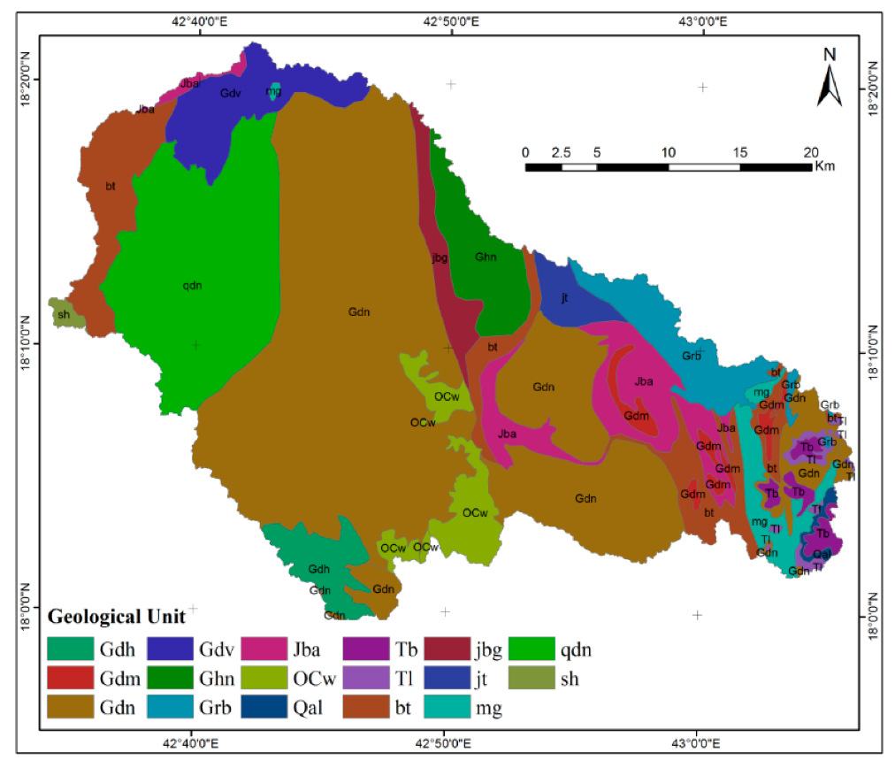
| Head | Code | Description |
|---|---|---|
| Dioritic and gabbroic rocks | sh | Shonkinite |
| mg | Metagabbro and gabbro-metagabbro (mg); mixture formed of gabbro sheets and irregular bodies within diorite (dgb) or within metamorphic rocks (mgy) | |
| Tonalite suite | qdn | Hornblende-biotite tonalite-gneissic tonalite (gdn); hornblende diorite associated with hornblende-biotite (di2) |
| Jiddah group | jt | Basalt-pillow lava and andesite-pillow lava, tuff, decite tuff, flow breccia, carbonaceous conglomeratic greywacke, phyllite, and interbedded subordinate |
| bt | Bahah group within the Tayyah belt-volcaniclastic graywacke; subordinate chert, slate, and conglomerate; carbonaceous shale and siltstone; minor interbedded basalt, andesite, and dacite | |
| Granodiorite and granite suite | ghn | Biotite-hornblende granodiorite-foliated |
| gdm | Muscovite-biotite granodiorite-gneissic | |
| gdn/gdv | Biotite granodiorite and monzogranite-foliated uniform body (gdn); mixture formed of irregular layers and bodies in amphibolite (gdv) | |
| Granite suite | grb | Biotite monzogranite-uniform body (grb); mixture formed of dikes, sheets, and irregular bodies within tonalite and trondhjemite (gt) or with diorite and gabbro (dg) |
| gdh | Biotite-hornblende granodiorite to monzonite grandiorite and granite suite | |
| Jiddah and baha groups undivided | jbg | Biotite-quartz-plagioclase granofels-subordinate amphibolite, anabiotite schist |
| jba | Biotite-quartz-plagioclase granofels-subordinate amphibolite, anabiotite schist | |
| Sedimentary, volcanic, and metamorphic rocks | qal | Alluvial and gravel- includes fan deposits near tertiary basalt |
| O€w | Wajid sandstone | |
| tb | Tertiary basalt | |
| ti | Tertiary laterite |
| GEOl | SLP | R | TE | LD | DD | LULC | PSW | VC | TWI | K | ST | |
|---|---|---|---|---|---|---|---|---|---|---|---|---|
| GEOl | 1,1,1, | 1,3,5 | 1,3,5 | 1,3,5 | 3,5,7 | 3,5,7 | 3,5,7 | 3,5,7 | 5,7,9 | 5,7,9 | 7,9,11 | 7,9,11 |
| SLP | 1/5,1/3,1/1 | 1,1,1, | 1,3,5 | 1,3,5 | 3,5,7 | 3,5,7 | 3,5,7 | 3,5,7 | 5,7,9 | 5,7,9 | 5,7,9 | 7,9,11 |
| R | 1/5,1/3,1/1 | 1/5,1/3,1/1 | 1,1,1, | 1,1,1, | 1,3,5 | 1,3,5 | 1,3,5 | 3,5,7 | 3,5,7 | 3,5,7 | 3,5,7 | 5,7,9 |
| TE | 1/5,1/3,1/1 | 1/5,1/3,1/1 | 1,1,1, | 1,1,1, | 1,1,1, | 1,3,5 | 1,3,5 | 1,3,5 | 3,5,7 | 3,5,7 | 5,7,9 | 7,9,11 |
| LD | 1/7,1/5,1/3 | 1/7,1/5,1/3 | 1/5,1/3,1/1 | 1,1,1, | 1,1,1, | 1,1,1, | 1,3,5 | 1,3,5 | 1,3,5 | 3,5,7 | 3,5,7 | 5,7,9 |
| DD | 1/7,1/5,1/3 | 1/7,1/5,1/3 | 1/5,1/3,1/1 | 1/5,1/3,1/1 | 1,1,1, | 1,1,1, | 1,1,1, | 1,3,5 | 1,3,5 | 3,5,7 | 3,5,7 | 5,7,9 |
| LULC | 1/7,1/5,1/3 | 1/7,1/5,1/3 | 1/5,1/3,1/1 | 1/5,1/3,1/1 | 1/5,1/3,1/1 | 1,1,1, | 1,1,1, | 1,1,1, | 1,3,5 | 3,5,7 | 3,5,7 | 5,7,9 |
| PSW | 1/7,1/5,1/3 | 1/7,1/5,1/3 | 1/7,1/5,1/3 | 1/5,1/3,1/1 | 1/5,1/3,1/1 | 1/5,1/3,1/1 | 1,1,1, | 1,1,1, | 1,1,1, | 1,3,5 | 3,5,7 | 5,7,9 |
| VC | 1/9,1/7,1/5 | 1/9,1/7,1/5 | 1/7,1/5,1/3 | 1/7,1/5,1/3 | 1/5,1/3,1/1 | 1/5,1/3,1/1 | 1/5,1/3,1/1 | 1,1,1, | 1,1,1, | 1,1,1, | 1,3,5 | 3,5,7 |
| TWI | 1/9,1/7,1/5 | 1/9,1/7,1/5 | 1/7,1/5,1/3 | 1/7,1/5,1/3 | 1/7,1/5,1/3 | 1/7,1/5,1/3 | 1/7,1/5,1/3 | 1/5,1/3,1/1 | 1,1,1, | 1,1,1, | 1,3,5 | 3,5,7 |
| K. | 1/11,1/9,1/7 | 1/9,1/7,1/5 | 1/7,1/5,1/3 | 1/9,1/7,1/5 | 1/7,1/5,1/3 | 1/7,1/5,1/3 | 1/7,1/5,1/3 | 1/7,1/5,1/3 | 1/5,1/3,1/1 | 1/5,1/3,1/1 | 1,1,1, | 1,3,5 |
| ST | 1/11,1/9,1/7 | 1/11,1/9,1/7 | 1/9,1/7,1/5 | 1/11,1/9,1/7 | 1/9,1/7,1/5 | 1/9,1/7,1/5 | 1/9,1/7,1/5 | 1/9,1/7,1/5 | 1/7,1/5,1/3 | 1/7,1/5,1/3 | 1/5,1/3,1/1 | 1,1,1, |
| GEOl | SLP | R | TE | LD | DD | LULC | |||||||||||||||
| GEOl | 0.271 | 0.300 | 0.274 | 0.271 | 0.300 | 0.274 | 0.272 | 0.301 | 0.274 | 0.272 | 0.301 | 0.274 | 0.271 | 0.300 | 0.274 | 0.271 | 0.300 | 0.274 | 0.271 | 0.300 | 0.274 |
| SLP | 0.185 | 0.209 | 0.195 | 0.186 | 0.209 | 0.195 | 0.186 | 0.209 | 0.195 | 0.186 | 0.209 | 0.195 | 0.186 | 0.209 | 0.195 | 0.186 | 0.209 | 0.195 | 0.186 | 0.209 | 0.195 |
| R | 0.104 | 0.101 | 0.125 | 0.104 | 0.101 | 0.125 | 0.104 | 0.101 | 0.125 | 0.104 | 0.101 | 0.125 | 0.104 | 0.101 | 0.125 | 0.104 | 0.101 | 0.125 | 0.104 | 0.101 | 0.125 |
| TE | 0.100 | 0.092 | 0.114 | 0.100 | 0.093 | 0.114 | 0.100 | 0.093 | 0.114 | 0.100 | 0.093 | 0.114 | 0.100 | 0.093 | 0.114 | 0.100 | 0.093 | 0.114 | 0.100 | 0.093 | 0.114 |
| LD | 0.070 | 0.062 | 0.061 | 0.070 | 0.062 | 0.061 | 0.070 | 0.062 | 0.061 | 0.070 | 0.062 | 0.061 | 0.070 | 0.062 | 0.061 | 0.070 | 0.062 | 0.061 | 0.070 | 0.062 | 0.061 |
| DD | 0.057 | 0.052 | 0.055 | 0.057 | 0.052 | 0.055 | 0.057 | 0.052 | 0.055 | 0.057 | 0.052 | 0.055 | 0.057 | 0.052 | 0.055 | 0.057 | 0.052 | 0.055 | 0.057 | 0.052 | 0.055 |
| LULC | 0.052 | 0.047 | 0.051 | 0.052 | 0.047 | 0.051 | 0.052 | 0.047 | 0.051 | 0.052 | 0.047 | 0.051 | 0.052 | 0.047 | 0.051 | 0.052 | 0.047 | 0.051 | 0.052 | 0.047 | 0.051 |
| PSW | 0.045 | 0.041 | 0.043 | 0.045 | 0.041 | 0.043 | 0.045 | 0.041 | 0.043 | 0.045 | 0.041 | 0.043 | 0.045 | 0.041 | 0.043 | 0.045 | 0.041 | 0.043 | 0.045 | 0.041 | 0.043 |
| VC | 0.033 | 0.029 | 0.028 | 0.033 | 0.029 | 0.028 | 0.033 | 0.029 | 0.028 | 0.033 | 0.029 | 0.028 | 0.033 | 0.029 | 0.028 | 0.033 | 0.029 | 0.028 | 0.033 | 0.029 | 0.028 |
| TWI | 0.030 | 0.027 | 0.024 | 0.030 | 0.027 | 0.024 | 0.030 | 0.027 | 0.024 | 0.030 | 0.027 | 0.024 | 0.030 | 0.027 | 0.024 | 0.030 | 0.027 | 0.024 | 0.030 | 0.027 | 0.024 |
| K. | 0.024 | 0.021 | 0.018 | 0.024 | 0.021 | 0.018 | 0.025 | 0.021 | 0.018 | 0.024 | 0.021 | 0.018 | 0.024 | 0.021 | 0.018 | 0.024 | 0.021 | 0.018 | 0.024 | 0.021 | 0.018 |
| ST | 0.021 | 0.018 | 0.014 | 0.021 | 0.018 | 0.014 | 0.021 | 0.018 | 0.014 | 0.021 | 0.018 | 0.014 | 0.021 | 0.018 | 0.014 | 0.021 | 0.018 | 0.014 | 0.021 | 0.018 | 0.014 |
| PSW | VC | TWI | K | ST | l | m | n | Defuzzify | Weight | ||||||||||||
| GEOl | 0.272 | 0.300 | 0.274 | 0.271 | 0.300 | 0.274 | 0.271 | 0.300 | 0.274 | 0.272 | 0.300 | 0.274 | 0.272 | 0.301 | 0.274 | 0.271 | 0.300 | 0.274 | 0.282 | 28.24 | |
| SLP | 0.186 | 0.209 | 0.195 | 0.186 | 0.209 | 0.195 | 0.186 | 0.209 | 0.195 | 0.186 | 0.209 | 0.195 | 0.186 | 0.209 | 0.195 | 0.186 | 0.209 | 0.195 | 0.197 | 19.72 | |
| R | 0.104 | 0.101 | 0.125 | 0.104 | 0.101 | 0.125 | 0.104 | 0.101 | 0.125 | 0.104 | 0.101 | 0.125 | 0.104 | 0.101 | 0.125 | 0.104 | 0.101 | 0.125 | 0.110 | 11.02 | |
| TE | 0.100 | 0.093 | 0.114 | 0.100 | 0.093 | 0.114 | 0.100 | 0.093 | 0.114 | 0.100 | 0.093 | 0.114 | 0.100 | 0.093 | 0.114 | 0.100 | 0.093 | 0.114 | 0.102 | 10.24 | |
| LD | 0.070 | 0.062 | 0.061 | 0.070 | 0.062 | 0.061 | 0.070 | 0.062 | 0.061 | 0.070 | 0.062 | 0.061 | 0.070 | 0.062 | 0.061 | 0.070 | 0.062 | 0.061 | 0.064 | 6.45 | |
| DD | 0.057 | 0.052 | 0.055 | 0.057 | 0.052 | 0.055 | 0.057 | 0.052 | 0.055 | 0.057 | 0.052 | 0.055 | 0.057 | 0.052 | 0.055 | 0.057 | 0.052 | 0.055 | 0.055 | 5.48 | |
| LULC | 0.052 | 0.047 | 0.051 | 0.052 | 0.047 | 0.051 | 0.052 | 0.047 | 0.051 | 0.052 | 0.047 | 0.051 | 0.052 | 0.047 | 0.051 | 0.052 | 0.047 | 0.051 | 0.050 | 4.99 | |
| PSW | 0.045 | 0.041 | 0.043 | 0.045 | 0.041 | 0.043 | 0.045 | 0.041 | 0.043 | 0.045 | 0.041 | 0.043 | 0.045 | 0.041 | 0.043 | 0.045 | 0.041 | 0.043 | 0.043 | 4.29 | |
| VC | 0.033 | 0.029 | 0.028 | 0.033 | 0.029 | 0.028 | 0.033 | 0.029 | 0.028 | 0.033 | 0.029 | 0.028 | 0.033 | 0.029 | 0.028 | 0.033 | 0.029 | 0.028 | 0.030 | 3.00 | |
| TWI | 0.030 | 0.027 | 0.024 | 0.030 | 0.027 | 0.024 | 0.030 | 0.027 | 0.024 | 0.030 | 0.027 | 0.024 | 0.030 | 0.027 | 0.024 | 0.030 | 0.027 | 0.024 | 0.027 | 2.69 | |
| K. | 0.024 | 0.021 | 0.018 | 0.024 | 0.021 | 0.018 | 0.024 | 0.021 | 0.018 | 0.024 | 0.021 | 0.018 | 0.024 | 0.021 | 0.018 | 0.024 | 0.021 | 0.018 | 0.021 | 2.13 | |
| ST | 0.021 | 0.018 | 0.014 | 0.021 | 0.018 | 0.014 | 0.021 | 0.018 | 0.014 | 0.021 | 0.018 | 0.014 | 0.021 | 0.018 | 0.014 | 0.021 | 0.018 | 0.014 | 0.018 | 1.75 | |
| Sl. No | Theme | Theoretical Weight (%) | Effective Weight (%) | |||
|---|---|---|---|---|---|---|
| Min. | Max. | Mean | Std. Dev. | |||
| 1 | GEOl | 28.24 | 5.10 | 64.20 | 31.33 | 10.131 |
| 2 | SLP | 19.72 | 1.65 | 55.33 | 20.56 | 8.982 |
| 3 | R | 11.02 | 4.06 | 38.84 | 10.94 | 5.011 |
| 4 | TE | 10.24 | 0.03 | 37.90 | 11.20 | 4.571 |
| 5 | LD | 6.45 | 0 | 18.43 | 5.90 | 2.321 |
| 6 | DD | 5.48 | 0 | 16.25 | 4.20 | 1.902 |
| 7 | LULC | 4.99 | 0 | 15.71 | 4.02 | 1.864 |
| 8 | PSW | 4.29 | 0.01 | 17.82 | 3.52 | 2.059 |
| 9 | VC | 3.00 | 0 | 6.26 | 2.06 | 0.474 |
| 10 | TWI | 2.69 | 1.42 | 5.85 | 1.20 | 0.519 |
| 11 | K | 2.13 | 0.01 | 6.83 | 2.34 | 0.817 |
| 12 | ST | 1.75 | 0.54 | 7.14 | 2.73 | 0.716 |
| Sl. No | Zones of GWPZ | GWPI (Range) | Area | % of Total Area | Existing Well Locations | % of Total Existing Well |
|---|---|---|---|---|---|---|
| 1 | Very poor GWPZ | 0.17–0.30 | 110.86 | 9.17 | 2 | 1 |
| 2 | Poor GWPZ | 0.31–0.46 | 243.75 | 20.18 | 11 | 5 |
| 3 | Moderate GWPZ | 0.47–0.52 | 329.53 | 27.28 | 31 | 13 |
| 4 | Good GWPZ | 0.53–0.59 | 347.69 | 28.78 | 55 | 23 |
| 5 | Very good GWPZ | 0.60–0.80 | 176.22 | 14.59 | 140 | 59 |
| Total | 1208 | 100 | 240 | 100 | ||
© 2019 by the authors. Licensee MDPI, Basel, Switzerland. This article is an open access article distributed under the terms and conditions of the Creative Commons Attribution (CC BY) license (http://creativecommons.org/licenses/by/4.0/).
Share and Cite
Mallick, J.; Khan, R.A.; Ahmed, M.; Alqadhi, S.D.; Alsubih, M.; Falqi, I.; Hasan, M.A. Modeling Groundwater Potential Zone in a Semi-Arid Region of Aseer Using Fuzzy-AHP and Geoinformation Techniques. Water 2019, 11, 2656. https://doi.org/10.3390/w11122656
Mallick J, Khan RA, Ahmed M, Alqadhi SD, Alsubih M, Falqi I, Hasan MA. Modeling Groundwater Potential Zone in a Semi-Arid Region of Aseer Using Fuzzy-AHP and Geoinformation Techniques. Water. 2019; 11(12):2656. https://doi.org/10.3390/w11122656
Chicago/Turabian StyleMallick, Javed, Roohul Abad Khan, Mohd Ahmed, Saeed Dhafer Alqadhi, Majed Alsubih, Ibrahim Falqi, and Mohd Abul Hasan. 2019. "Modeling Groundwater Potential Zone in a Semi-Arid Region of Aseer Using Fuzzy-AHP and Geoinformation Techniques" Water 11, no. 12: 2656. https://doi.org/10.3390/w11122656