Sewer Life Span Prediction: Comparison of Methods and Assessment of the Sample Impact on the Results

Abstract

Survival models can support the estimation of the resources needed for future renovations of sewer systems. They are particularly useful, when a large share of network will need renovation. This paper studies modelling sewer deterioration in a context, where data are available for pipes selected for inspections due to suspected or experienced poor condition. We compare the random survival forest and the Weibull regression for modelling survival and find that both methods yield similar results, but the random survival forest performs slightly better. We propose a method for estimating the range in which the actual network survival curve lies. We conclude that in order to reach reliable results, a life span model needs to be constructed based on a random sample of pipes, which are then consecutively inspected and in addition, censoring and left truncation need to be accounted for. The inspection data applied in this paper had been collected with the aim of finding pipes in poor condition in the network. As a result, the data were biased towards poor condition and unrepresentative in terms of pipe ages.

1. Introduction

The majority of the sewer systems in Finland have been built in the 1970s or after [1]. Some of the country’s networks have already been renewed, but mainly, the systems are just entering the phase where extensive renovation is needed. Models that predict the evolution of network condition into the future provide support for optimal investment and rehabilitation planning of sewer networks [2] and water and wastewater utilities could potentially benefit from these models. In particular, the models can support utilities in mid- and long-term asset management decisions in cases where the information on network condition is limited [3].

Survival models are so-called time-to-event models, which provide a means to determine the distribution of time until an event of interest occurs. They differ from some other statistical modelling methods in the respect that they account for censoring [4]. They are therefore suitable for estimating, for example, the useful life of sewers. The methods existing for survival estimation can be divided into parametric, semi-parametric, and non-parametric categories [4]. The parametric methods are based on assumptions made on the probability distribution of the survival times. The parameter values are determined so that they best fit the data. A good number of possible distributions exists, for example, the exponential [5,6], Weibull [6,7], Herz [8], and Gompertz [3,9,10] distributions have all been applied in sewer deterioration modelling. The Cox proportional hazards model [11] is a semi-parametric model, where the hazard function is estimated non-parametrically, but the effect of the predictors on the hazard function is assumed to be parametric. The non-parametric models cover, for example, life-table estimates and the Kaplan–Meier method [4]. Additionally, there are machine learning methods such as random survival forest and support vector machines.

It is common that sewer condition data is subject to right and left censoring and possibly interval censoring and left truncation [12]. Right censoring means that, at the time of the inspection, the event of interest, for example the worst condition class, was not yet observed [13]. Left censoring, on the other hand, denotes a case where the event of interest has already occurred at the time of observation [13]. For example, a pipe is found to be in the worst condition class but it is unclear, at which point in time the class was entered. In case a pipe has been inspected twice and the condition state has changed between the inspections, interval censoring is present, since the exact moment of the transition from one condition state to the next one is unknown [13]. Left truncation is present, when some objects have already experienced the event of interest, but the point in time is unknown and they are not included in the study [14]. In sewers, this would be the case where some pipes have already been decommissioned and the information on the decommissioning time and pipe condition are missing.

Different types of Markov chains have frequently been applied for sewer deterioration modelling. The homogeneous Markov model is a time-homogeneous model, where the probability of moving from the current condition state to the next one only depends on the present condition state, regardless of the preceding condition states or the time spent in them. In the non-homogenous Markov model, transition probabilities are time dependent. In the semi-Markov model, the condition state depends also on the time spent in the given state, but the model is still independent of the path by which the present state was reached [15]. Markov chains are especially suitable for situations, where the data allows modelling the transition from one condition state to the next one. Other multi-state models include the so-called cohort model [8], where a different curve is created for each group of pipes, a cohort.

Wirahadikusumah et al. [5] and Micevski et al. [16] were early appliers of homogeneous Markov models, which were later also applied by Baik et al. [17] and Dirksen and Clemens [18]. Wirahadikusumah et al. [5] calibrated the transition curves using exponential regression, while Micevski et al. [16] applied a Bayesian approach. Baik et al. [17] estimated the transition probabilities using an ordered probit model and Dirksen and Clemens [18] using maximum likelihood estimation. Weibull distribution was applied by Mailhot et al. [7] and the Herz distribution by Baur and Herz [8]. Le Gat [10] applied the so-called GompitZ model, where the evolution of condition is modeled using non-homogenous Markov chains and the survival times follow the Gompertz distribution. El-Housni et al. [19] applied Cox regression and likelihood ratio test in modelling structural deterioration.

Even though Micevski et al. [16] validated their model in 2002, it has only been more recently that model validation and assessment of model limitations have gained more attention. In 2014, Rokstad et al. [9] assessed how sensitive the GompitZ model is on the amount of inspection data and whether it is possible to assess this uncertainty in a case where the data set is incomplete. They applied Monte Carlo simulations and found that even when 40–60% of the network has been inspected and the analysis is based on a random sample, the uncertainties may be considerable. They found that there was uncertainty relating to both predicting the overall condition distribution of the network and the state of individual pipes. Rokstad and Ugarelli [20] compared the predictions given by the GompitZ model and a random forest (RF) model and found that RF generally outperformed GompitZ in terms of uncertainty. However, when the amount of data was reduced, both predictions exhibited clear biases. In contrast, when Caradot et al. [3] applied the GompitZ model, their finding was that GompitZ was capable of creditably predicting the amount of pipes in poor condition using only 3% of data for model calibration (about 1000 pipes). Moreover, Duchesne et al. [6] found that even small sizes of random samples were enough to produce applicable deterioration curves. Scheidegger et al. [2] assessed the effects of deterioration, replacement policy, and expansions of the sewer network on the modelling results. Their method can be used to quantify the effect of missing or uncertain data. Even though they do not state it explicitly, it is clear that this result is based on a random sample. They found that if historical data are missing, the model might overestimate the average life expectancy by up to 200 years. Indeed, the useful lives either based on handbook values or estimated in different studies vary greatly (see for example [16,19,21]). Furthermore, Scheidegger and Maurer [22] found that the uncertainties related to the parameters of the Herz model were significant in the case of young sewer systems with fewer pipes in poor condition, while the Markov model was less affected by this phenomenon. Later, Egger et al. [23] proposed a method for calibrating a sewer deterioration model when some of the historical condition data are lacking. Duchesne et al. [6] proposed a method for accounting for both left and right censoring in a survival model. They applied exponential and Weibull distributions in modelling the waiting times in the different condition stages.

Limitations in data availability, applicability, and quality are common in sewer condition data. Sewer pipes are very sparsely inspected infrastructure (Le Gat [10]) and in many cases, assessing and validating the deterioration models is difficult due to the lack of reliable data (Scheidegger and Maurer [22]). The importance of sample representativeness has been brought out in previous research (Le Gat, 2008 [10]; Duchesne et al., [6]). For example, Le Gat [10] notes that having longitudinal data is likely to improve the usefulness of the results. However, in practice, the inspected set of pipes often consists of recently installed pipes or pipes assumed to be in poor condition (Le Gat [10]), which causes a selection bias. To overcome this obstacle, some studies have used simulated data (Scheidegger et al., [2]; Scheidegger and Maurer, [22]). In cases where actual data were applied, their extent and characteristics varied. In Rokstad and Ugarelli [20], the data set comprised some 27% of the Oslo VAV sewer network, mainly inspected within a five years period. Caradot et al. [3] had an extensive data set where all the network pipes had been inspected at least once and more than 50% at least twice. Data on pipes that had been replaced before the start of the data collection, however, were missing. The study by Duchesne et al. [24] highlights the importance of data availability. They found that the annual replacement rate needed to maintain the share of pipes in a poor condition on the desired level was three times less in a case where the condition of all network pipes was known, compared to a situation where the condition was unknown for all pipes.

The tradition of validating the sewer survival models is not very strong and the goodness-of-fits of the reported cases vary greatly. The most common way of validation has been testing the model’s predictive power on a validation data set. This was done in Micevski et al. [16], who also applied chi-squared tests to determine the validity of the model and the influence of the explanatory variables. Baik et al. [17] applied the likelihood ratio index as a measure for the goodness-of-fit for each transition, but found the fit to be rather low (maximum 0.28). In the study by Duchesne et al. [6] an exponential model produced robust results despite the sample being small and having some differences compared to the whole network. The material used for model creation consisted of inspection results for some 22% of the network.

Support vector machines [25,26], decision trees [25], and random forests [27] have been applied in estimating sewer pipe condition (for example [25,26]), but to our knowledge, machine learning methods have been applied in survival estimation only in such fields as medicine.

The offset for the present analysis has been to study, how well a typically available data set lends itself to deterioration modelling. We tested Markov models, but found the input data unsuitable for them for two reasons. Firstly, no clear evolution of condition from one condition state to the next poorer one was detectable in the data. Secondly, there was only one inspection result available for each pipe, which is not in line with the original purpose of multi-stage models [12]. Instead of modelling the evolution of condition, we compare two different survival methods for estimating the time to the age when pipes need renovation. The aim of creating a survival model is to provide support for the estimation of the resources needed for future renovations. We study how useful the created survival models are in a context where the data set consists of pipes selected for inspections. We propose a method for a rough estimate on the range of the intervention age based on a sample where pipes in poor condition are over-represented. Section 2 describes the data set used for the analysis and presents the Weibull and random survival forest methods for survival estimation. It describes the methods applied for estimating model goodness-of-fit and comparing the models. It also outlines the procedure for estimating the optimistic and pessimistic life span curves from the data. Section 3 presents the created survival curves and compares them. Section 4 highlights the possible reasons to the differences between estimated life spans in various studies and discusses how the sample affects the results. Section 5 puts together the main findings related to method selection and the use of CCTV (closed-circuit television) inspection results in deterioration modelling.

2. Materials and Methods

2.1. Network Information and the Inspection Data Set

The studied foul sewer network is located in Southern Finland. The oldest pipes in the network date from the year 1955 and until now the network has experienced a great expansion and has currently a total length of ca. 1200 km. Between the years 2001 and 2016, approximately 30% of the network was CCTV inspected. Approximately 12% of the inspections concerned pipes that had been replaced between 2001 and 2016. In addition, some pipes had been replaced prior to the start of the data collection, although no extensive renovation had taken place before the starting of the CCTV inspection data collection in 2001. The utility company has selected pipes for inspections based on expert judgement, mainly covering three reasons: (1) The utility suspects that an area needs renovation and inspects all pipes in the area; (2) the inspection is carried out to find out the reason to an operational problem such as blockage; or (3) a pipe is inspected at the end of the guarantee period.

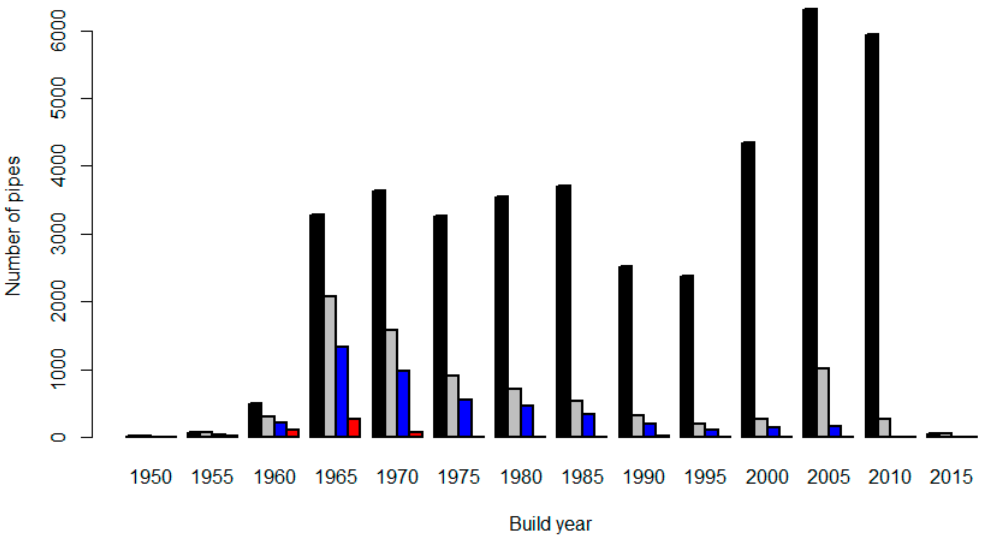
Only gravitational pipes and the largest material groups were considered. We removed records with clearly erroneous attributes, e.g., pipes with a negative pipe age at the time of inspection or installation depth smaller than 0.5 m or higher than 4 m. Figure 1 shows the distribution of pipe build years in the complete network, in the inspected network, and in the final data set after removing pipes with erroneous or missing attributes (both training and validation data together).

Figure 1 illustrates how the data set represents best the pipes that were built before the year 1990. The network has expanded after the year 2000 but, understandably, there are far fewer inspection results for these relatively new pipes. It is also likely that for the newer pipes, the reason for the inspection was an operational problem, which makes these pipes represent poorly their own age category. Creating a representative set of pipes with respect to their installation year is impossible due to the low number of inspections in the newest pipes. Moreover, the high number of explanatory variables would further complicate obtaining a sample fully representative of all variables. The set of explanatory factors included altogether 19 different variables covering pipe attributes (for example, installation year, material, slope, pipe end coordinates), environmental attributes (for example soil type, location with respect to road), and network-related attributes (pipe-specific annual sewage flow). The attributes are presented in more detail in [27].

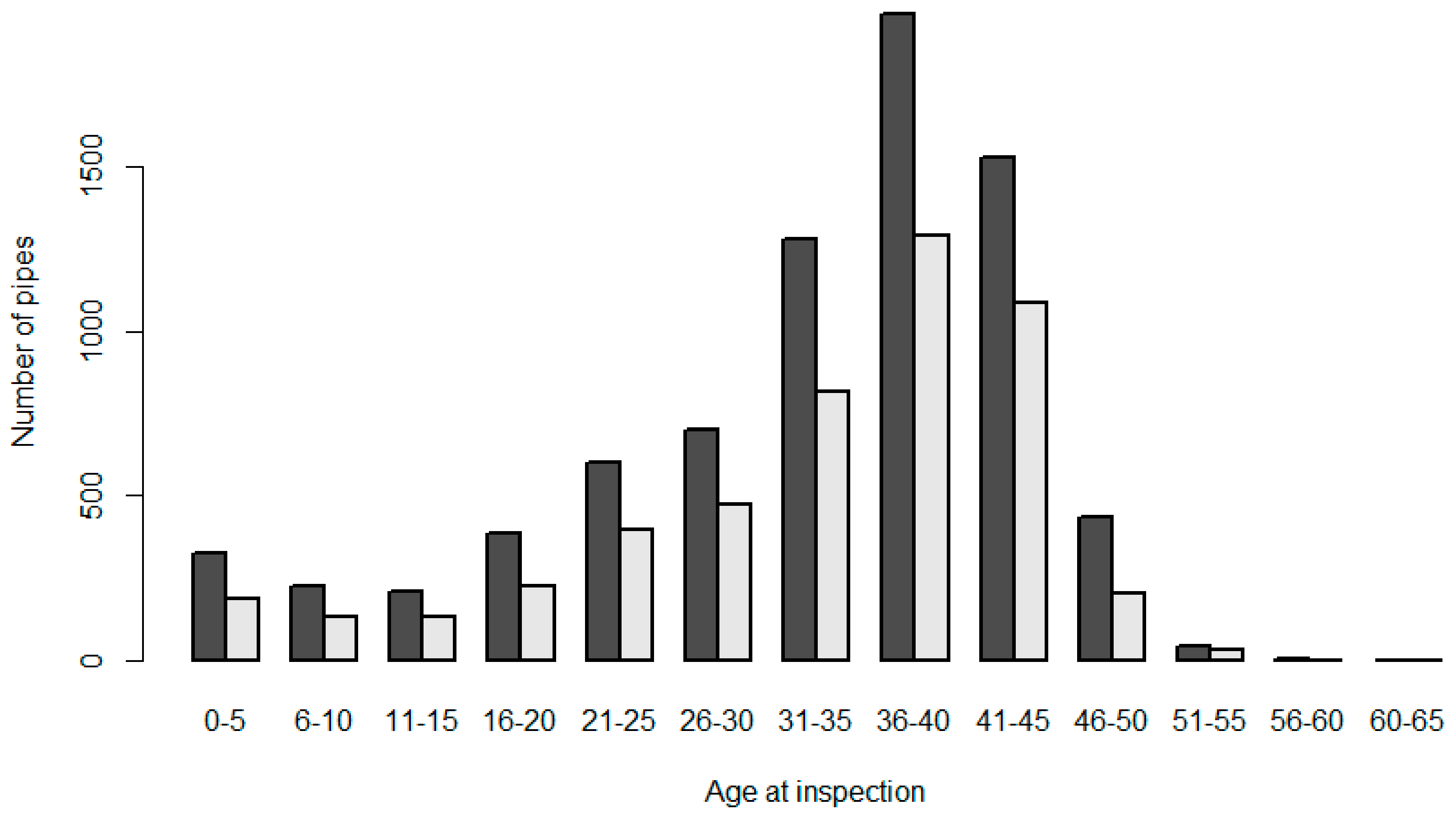
Figure 2 presents the age distribution of the inspected pipes at the time of the inspection.

Figure 2 illustrates how the age distribution remains similar even after data pre-processing. It also demonstrates how the majority of the inspected pipes have been inspected around the age of 40 years.

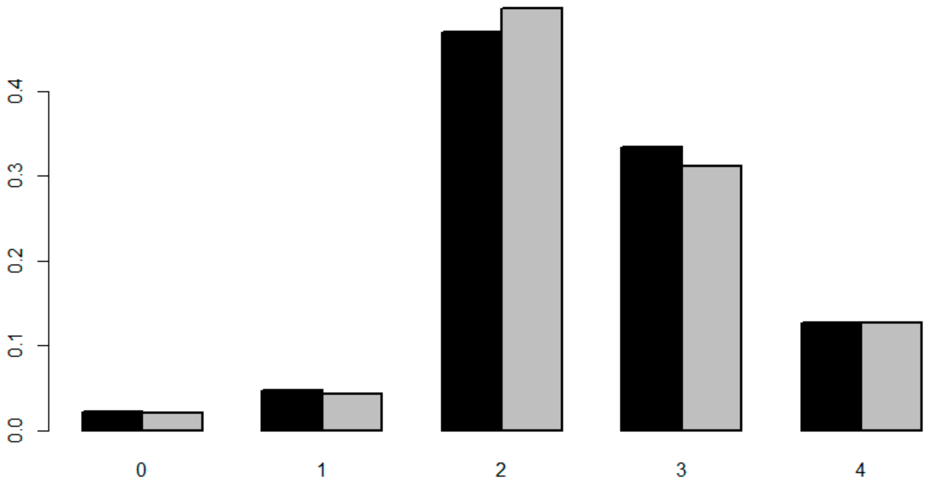
The complete inspection data included ca. 48,000 observations for ca. 10,000 pipes. After the removal of pipes with missing or erroneous attributes, the final data set comprised ca. 4500 pipes. The scoring of the observations follows a five-step scale of the Finnish guidelines for sewer inspections, which are an application of the European standard EN-13508-2 (2003). Score 0 indicates no defect, 1 “slight defect”, 2 “minor defect”, 3 “moderate defect”, and 4 “serious defect”. Figure 3 illustrates the pipe maximum score distribution before and after the removal of pipes with missing or erroneous attributes.

Figure 3 shows how scores 0 and 1 form a small fraction in the data set, score 2 is the most common one and ca. 13% of the pipe maximum scores in the data set reached score 4. Even after the removal of erroneous data and pipes with missing attributes, the share of pipes in different condition states remains fairly similar. It seems reasonable to assume that the low share of pipes in a good condition in the data set results from a selection bias. Both expert judgement and the relatively young network age support this view.

We modeled the time when the pipe reaches condition class 4 to estimate the expected useful life. The data set is subject to right censoring, since not all pipes had reached state 4 at the time of the inspection and to left censoring, since the time for entering the worst condition state is unknown even for pipes where this condition was observed. To some extent, the data set also exhibits left truncation, since some of the network has been renovated prior to the start of the information collection, but accurate information on the renovated network lengths and pipe attributes was unavailable.

2.2. Survival Analysis with Weibull Regression and Random Survival Forest

We estimated the useful life of sewers using two methods: The Weibull regression model and the random survival forest. The random survival forest is a machine learning method for survival analysis, whereas the Weibull model is an established parametric method, where the survival times follow Weibull distribution. Both methods allow inclusion of covariates and account for right censoring. The aim was to compare the performance of a well-established statistical method such as Weibull regression with a less frequently applied machine learning method. Random survival forest was selected as the machine learning method due to the promising results gained in [27]. It was preferred over decision trees as it is not as prone to overfitting [28].

The survival function of the Weibull distribution is determined by two parameters: The shape parameter and the scale parameter. Different parameter values result in a wide variety of different shapes of survival functions, which makes the Weibull model very flexible. The Weibull distribution is also suitable for describing the survival distribution of a population with increasing, decreasing, or constant risk. More details on the method can be found in, for example, [4].

Random forest was originally developed in the early 2000s [29] for classification and was later extended to cover time-to-event analysis of right-censored data [30], the method being called random survival forest (RSF). For RSF, there are no restrictive assumptions on the model format and the difficulties related to possible nonlinear effects of variables are handled automatically. The core of the RSF method is in bootstrapping and random node splitting, which are applied when forming an ensemble of independent decision trees that form the RSF. Different splitting criteria such as log-rank and Harrel’s C can be applied. A detailed description of RSF is given in [30].

2.3. Assessment of the Predictive Power and the Goodness-Of-Fit of the Models

The predictive power and the goodness-of-fit of the two models were assessed using a validation data set and three metrics: The Brier score, the concordance index (c-index), and the share of correct predictions in the validation data set. The Brier score and the c-index are traditional measures for model performance and discriminative ability, respectively [31].

The Brier score [32] presents the accuracy of a survival prediction at a given time point t. The score expresses the squared distance between the actual survival outcome and the predicted survival probability. In a case where the data contains right censored events, the scores are adjusted by weighting the squared distances using the inverse probability-of-censoring weights method [33], which can be based on, for example, the Kaplan–Meier estimator. The prediction accuracy provided by the Brier score values can be followed over time to create a so-called prediction error curve. The Brier score values vary from 0 to 1, where 0 is the best possible value and 0.25 the highest possible value for a useful model [34]. The use of the Brier score has received some criticism [35,36] and should therefore be applied with caution, preferably together with other metrics.

In contrast to the Brier score, which measures the model fit, the c-index [37] is a well-established measure of the ranking ability of a time-to-event model and it is frequently applied in medical literature [38]. A pair of cases—here, a randomly chosen pair of pipes—is called concordant if the model predicts a higher risk of failure for a pipe that fails first. The c-index is the frequency of concordant pairs among the data set, it expresses, how often the predictor ranks correctly a pair of random observations. Again, in case the data contain right censored observations, the values must be weighed using the inverse probability-of-censoring and this can be based on, for example, the Kaplan–Meier estimate. The c-index for a perfect model is 1, whereas an arbitrary model receives a value of 0.5.

In addition to the two methods, the predictive power of the models was assessed against a validation data set in a similar fashion as in, for example, [3]. The model was trained with a subset comprising 70% of the original data and the remaining 30% was left for validation. The training data set consisted of ca. 3500 pipes and the validation data set of ca. 1000 pipes.

2.4. Estimating the Range of Network-Level Survival Curves

We propose a method for estimating the range where the whole network’s life span should settle. The estimates are made based on two contradicting assumptions that produce the boundaries for the range: The optimistic and the pessimistic survival curves. Since the majority of the data set results from pipes being suspected to be in poor condition, it would be reasonable to assume that the rest of the network is actually in a better condition than the pipes in the inspected sample. Therefore, the pessimistic estimate assumes that the selection of pipes for inspection has failed and the sample holds pipes approximately in the same condition as the rest of the network. By contrast, in the optimistic estimate, the selection of pipes for inspections is assumed to have succeeded fully and the sample is assumed to hold all pipes in poor condition in the whole network. We applied Weibull regression because it is able to predict beyond the age of the oldest pipe in the data set and explanatory variables are not necessarily needed for model creation. The optimistic curve was created with no explanatory variables, since not all variable values were available for the whole network.

3. Results

3.1. Comparison of Estimated Life Span Curves

Some of the 19 applied explanatory variables in the analysis were originally continuous, some categorical. Two options of variable values were tested; one, where continuous variables were kept continuous and another, where all explanatory variables were in a categorized form. For the RSF model the first option provided better results and for the Weibull model the latter one.

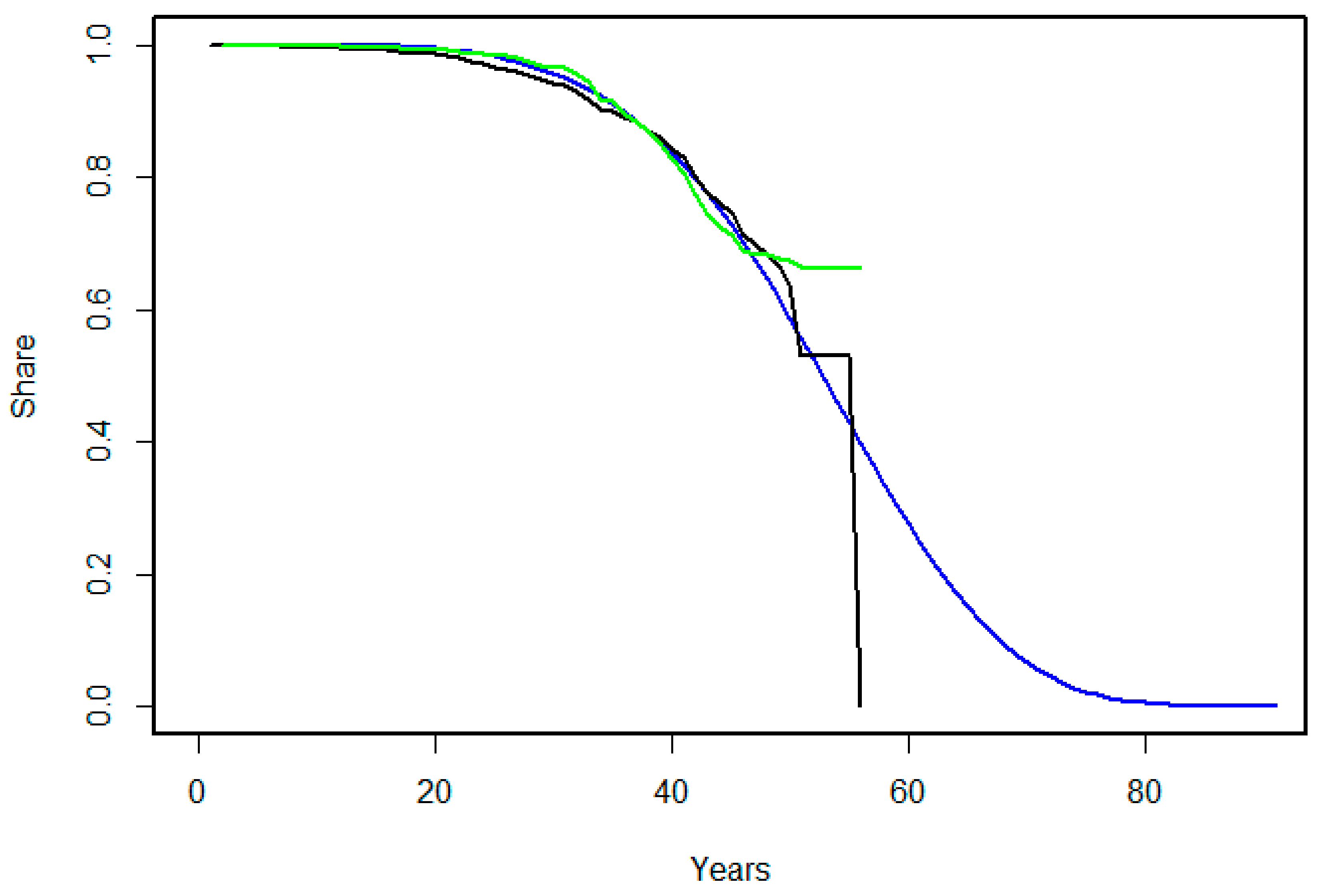
Figure 4 presents the life span curves created by the two models together with the Kaplan–Meier curve, which shows how the number of pipes still in useful condition evolves in the data set (For more information on the Kaplan–Meier curve see, for example, [13]).

Figure 4 shows, how the RSF and Weibull estimates result in similar-looking curves until approximately pipe age 50, where the two estimates diverge. The RSF and Weibull curves are similar to the Kaplan–Meier curve—the reason to why the Kaplan–Meier curve drops to 0 at the curve end is simply because the last observation is a single case of a pipe reaching the end of its life span. Both the RSF and the Weibull model estimate that by the age of 50, ca. 30% of the network has reached the end of its useful life. Since the Weibull model is a parametric model, it can predict beyond the age of the oldest inspected pipe and estimates that all the network will need renovation by the age of 85 years. Since RSF is not a parametric method, the estimate does not continue beyond the maximum pipe age of 56 years.

3.2. Goodness-Of-Fit and Predictive Power

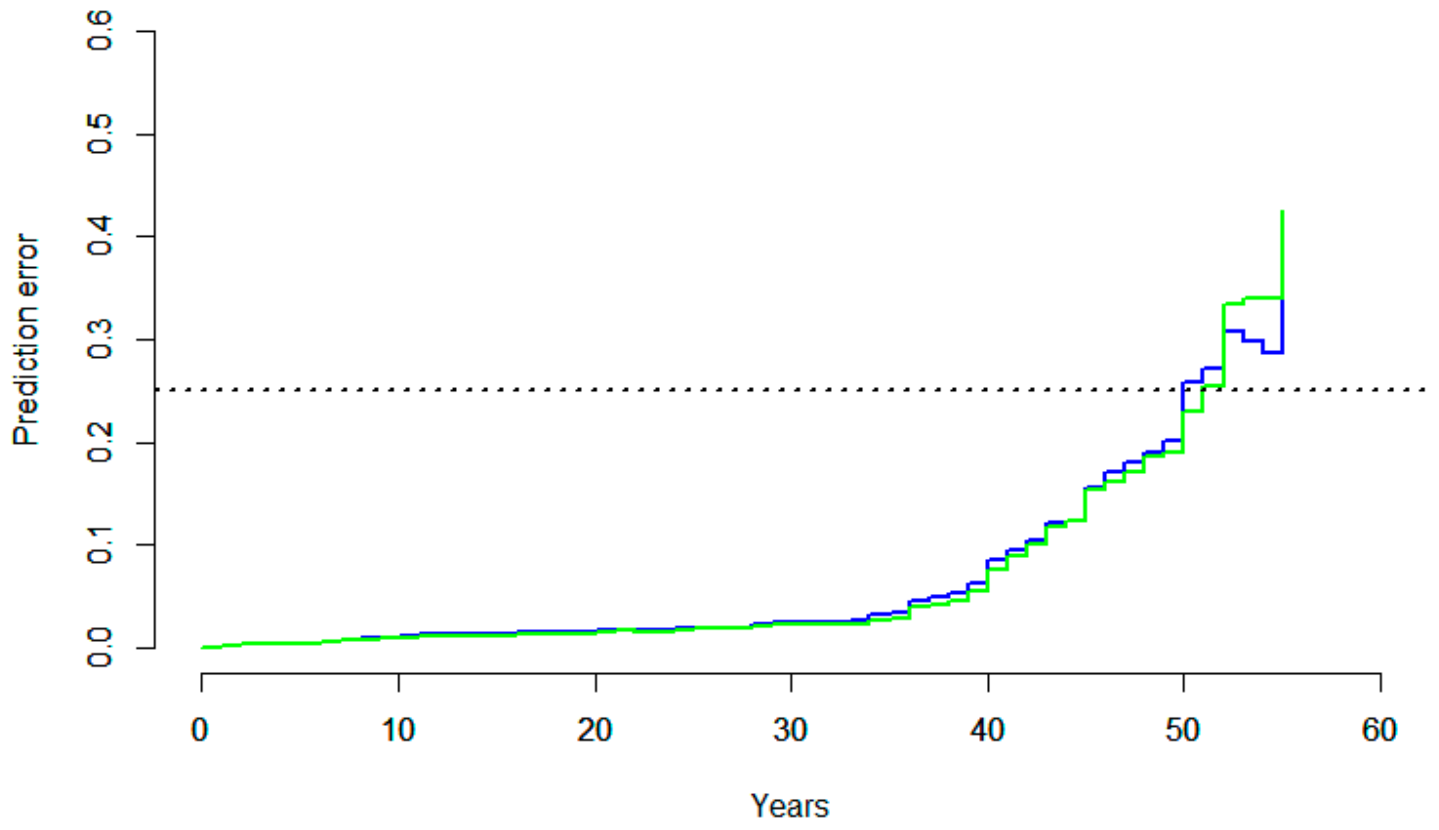
Figure 5 presents the Brier score values for the Weibull model (in blue) and the RSF model (in green).

Figure 5 illustrates how the two models perform very similarly and how the models become irrelevant at pipe ages 50 and above. The inverse probability-of-censoring weights were estimated using the Kaplan–Meier estimator for censoring times [33].

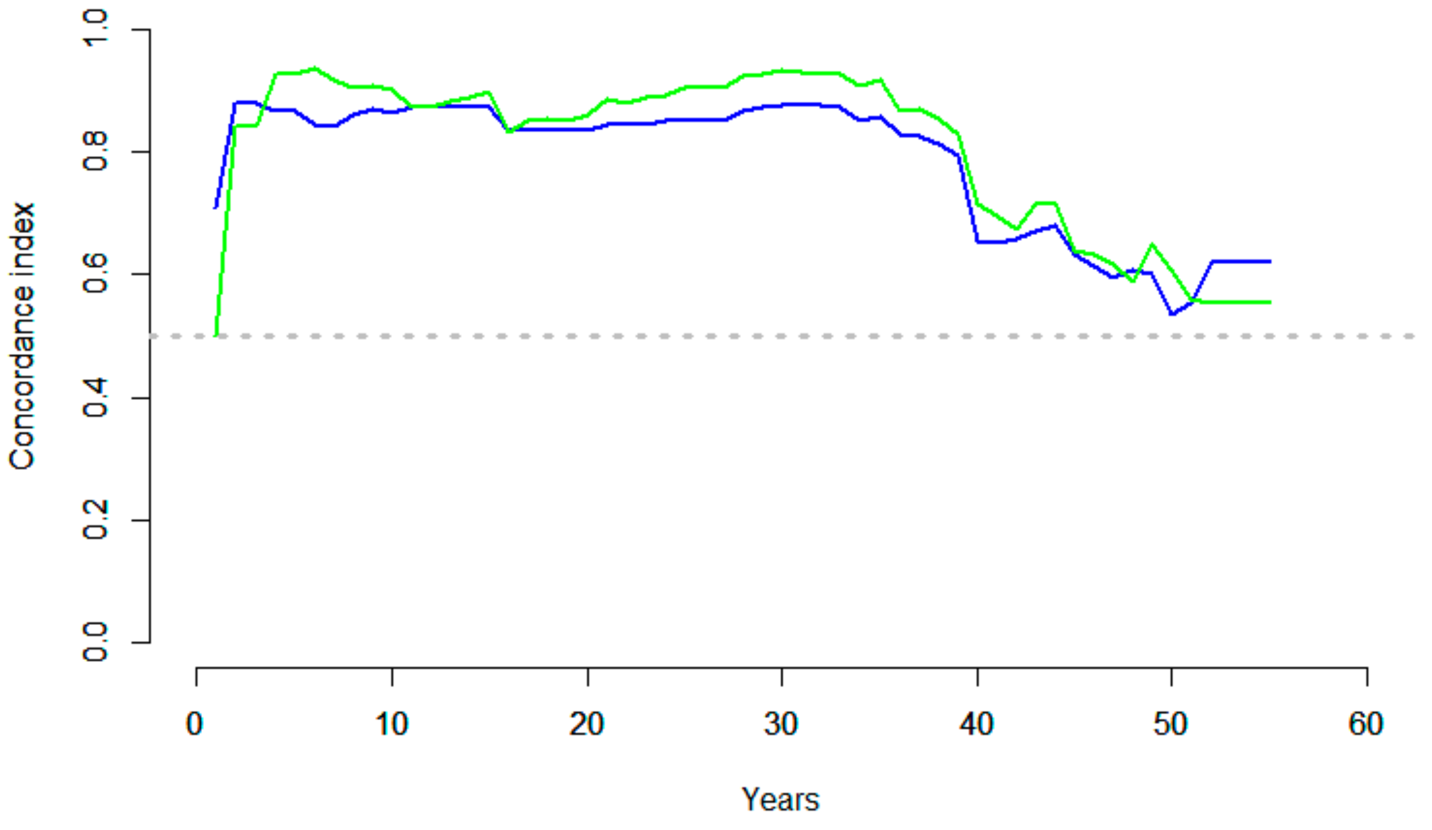
Figure 6 presents the c-indices for the two models at different time points. The Kaplan–Meier estimate was applied for weighing the observations with the inverse probability-of-censoring.

The c-index values were very similar for both models with predominantly values exceeding 0.8 until the pipe age of 35 years, where the model performance drops substantially. The RSF model performed slightly better apart from pipes of age three and younger and pipes of age 52 and older. The information provided by the c-index is in line with the prediction errors presented in Figure 5.

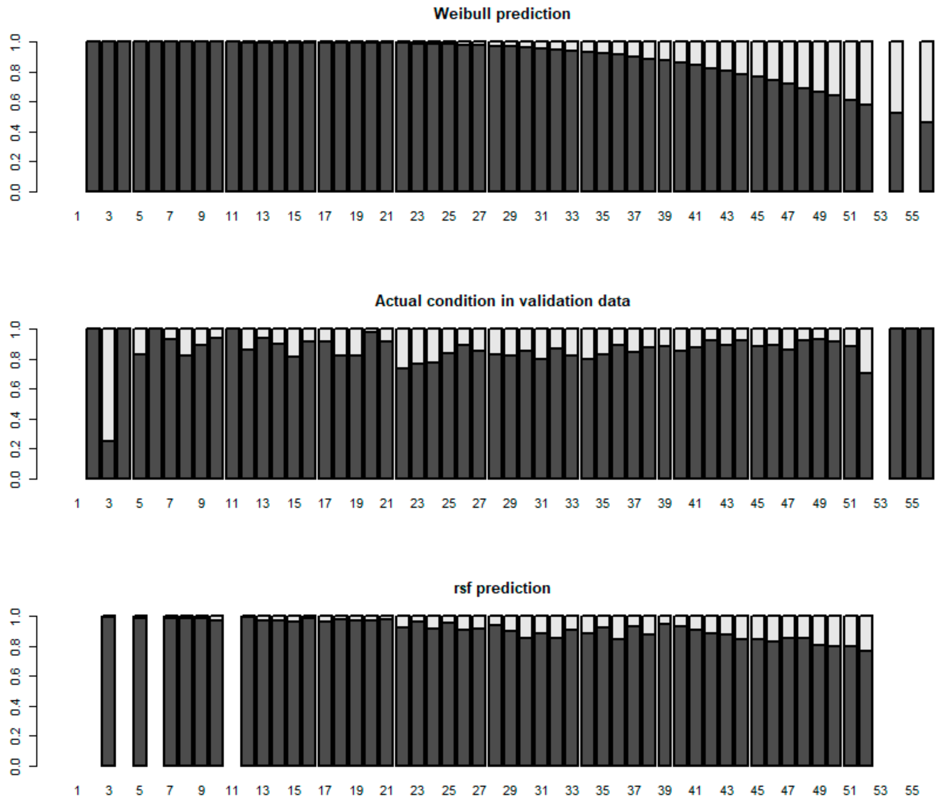
Moreover, the models’ predictive power was tested against a validation data set. Figure 7 shows the shares of pipes still in useful condition as a function of pipe age (1) as predicted by the Weibull model (top), (2) in the actual data set (middle), and (3) as predicted by the RSF model (bottom).

Figure 7 illustrates how the predictive accuracy of both models is relatively weak when assessed on an annual level. The actual condition distribution (middle) is somewhat surprising, showing little to no tendency towards poor condition with time. The RSF model (bottom) is able to capture some of this variation in the data, whereas the Weibull model (top) produces a credible-looking distribution, which only fits well for pipes of ages between 40 and 45 years, which is the age range where the majority of the pipes in the whole data set are. Both methods provide a fairly good prediction on the condition distribution in the validation data set, with the Weibull model overestimating the share of state four pipes by 10% and the RSF model underestimating it by 11%. However, when assessing pipes of a specific age group, the predicted shares differ from the observed shares up to 100%. The variability in the number of inspected pipes in different age categories complicates comparison of the information shown in the middle panel of Figure 7 with the survival curves presented in Figure 4. For example, at pipe ages 21–25 one could expect the survival curve in Figure 4 to show a steep decline, since in this age category the share of pipes at the end of the life span is higher than the average (Figure 7). However, as the number of pipes in this age category is low (Figure 2), the survival curve does not actually show such a behavior.

3.3. Optimistic and Pessimistic Estimates on the Real Life Span

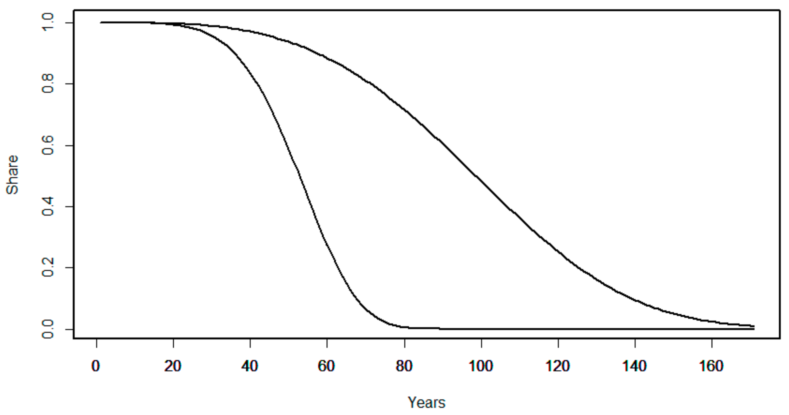
Figure 8 presents the estimated optimistic and pessimistic survival curves for the whole network. The pessimistic curve is the same as the Weibull curve in Figure 4. The optimistic curve has been created using the Weibull method on data with no explanatory variables.

The two life span curves show a difference of ca. 45 years in estimating the time when 50% of the network has reached the end of the life span: The estimate is approximately 55 years in the pessimistic case and approximately 100 in the optimistic case. In the pessimistic case, all pipes will need renovation by the age of 85, while the optimistic curve predicts the entire network will reach the end of useful life by the age of 170.

4. Discussion

The comparison of the RSF and the Weibull models revealed that both methods yielded very similar survival curves approximately until pipe age 50, after which the two estimates diverge. For pipe ages of 50 years and beyond, no strong conclusions on the curve fits can be made as only 2% of the data used for the model creation and validation represented pipes of this age. The comparison will provide more reliable results as more data will be collected over the years. The 70% survival is around 50 years for both curves and according to the Weibull curve all pipes are expected to reach the end of their useful life by the age of 85 years. These ages seem somewhat low and the likely reason lies in the sample, which is composed of pipes suspected or experienced to be in a poor condition. Moreover, the fact that deterioration with pipe age is not clearly visible in the data supports the view that the sample is not representative of the whole network. It is noteworthy that even in such a case creating a survival curve is possible, since the model presents the evolution of the share of pipes in good condition in the whole data set. According to the applied estimates for goodness-of-fit, RSF performed slightly better than the Weibull model, but the difference was very small. Both the prediction error and the c-index values provided similar results on the goodness-of-fit. When assessed from the perspective of predictive ability, neither of the models provided very good results. However, assessing the model goodness based on the predictive ability was also not highly informative due to the differences in the number of inspected pipes in different age groups. As the majority of pipes were of age between 30 and 45 years, the model fit is expected to be best for these age groups. This notion suggests that to produce reliable estimates of life span curves, the sample should be representative also in terms of pipe ages. The RSF model was easier to create as it functioned well even without the categorization of variable values as a preprocessing step. On the other hand, the RSF has the restrictions that it cannot be used to create a model without predictors and that it can only make predictions until the age of the oldest inspected pipe. However, in practice, the latter may be a fairly small limitation, since if survival models are used for planning the resourcing needed in the future, the 50% share, for example, will provide enough information to support those decisions.

In order to overcome the limitation of the sample, we created the optimistic and pessimistic curves to allow identifying the range where the actual survival curve should settle. Based on these, the true phase-out age of sewers in this network is estimated to lie between 85 and 170 years and the 50% share between 55 and 100 years. These ranges seem reasonable based on expert knowledge. The optimistic and pessimistic curves still pose two challenges: They do not incorporate left censoring nor left truncation. Left censoring is always present in an inspection data set and its practical consequence is that the curves are somewhat more optimistic than the reality. Even though the major renovation phase has started at late 1990s and the data set applied in this article contains information on the majority of the renovated pipes, the sample is also subject to left truncation. However, in a case where the sample is based on pipes selected for inspection, the young pipes in poor condition are likely to be overrepresented as well. Thus, the sample contains more long life spans due to left truncation and short life spans due to the sample having more pipes in poor condition than the rest of the network. To what extent these two effects compensate each other needs further study.

Egger et al. [23] note that when historical records are missing, the data set represents the combined effect of deterioration and rehabilitation. We would like to note that when the data consist of the inspected share of the network, the data set is also a result of the selection process of pipes for inspections.

The wide spectrum of life spans reported in the literature suggests that the field of modelling sewer pipe survival is still not fully mature. Scientific articles dealing with sewer condition also commonly present models on current condition and future deterioration together, although these require different models [4]. This hampers making conclusions, for example, on factors that affect deterioration. The literature review combined with the results presented here and in [27] support two conclusions: A sample where poor condition is overrepresented is more useful for condition prediction than it is for life span prediction. A random sample would be needed in order to predict life span reliably and even then, the possible left truncation needs to be dealt with, for example, by applying the method in [6].

In an ideal case, modelling of sewer life span should be based on panel data [39] on a representative sample. This would mean having separate campaigns for risk-based inspections, where the aim is to find pipes in poor condition or to discover the condition of critical pipes, and for collecting data for life span modelling. Until today, to the authors’ knowledge, only the risk-based inspections have been applied at Finnish utilities. A future challenge is to create inspection campaigns that yield reliable estimates for the future evolution of the network condition. A campaign like this should include a random sample of pipes inspected successively at least three times (as recommended by, for example, [5]). When analyzing the data, the modelling phase should consider the absence of information on pipes replaced earlier (if there are any), together with different types of censoring.

5. Conclusions

• Random survival forest provides a potential method for estimating sewer network deterioration. The RSF model performed slightly better than the Weibull model when assessed with the Brier score, c-index, and the predictive power on a validation data set. However, neither of the model provided excellent results, especially in the context of predictive ability.
• The optimistic and pessimistic life span curves provide a means of estimating the range of network life span based on a data set where pipes in poor condition are over-represented.
• A data set where pipes in poor condition are over-represented is more useful for finding pipes in poor condition in the whole network than for predicting future deterioration of the network.
• In order to make reliable life span estimates, the survival model needs to be created with a random sample of pipes inspected successively and the effect of right and left censoring and left truncation need to be considered.

References

- Lapinlampi, T.; Raassina, S. Vesihuoltolaitokset 1998–2000; Finnish Environment Institute: Helsinki, Finland, 2002. [Google Scholar]
- Scheidegger, A.; Hug, T.; Rieckermann, J.; Maurer, M. Network condition simulator for benchmarking sewer deterioration models. Water Res. 2011, 45, 4983–4994. [Google Scholar] [CrossRef] [PubMed]
- Caradot, N.; Sonnenberg, H.; Kropp, I.; Ringe, A.; Denhez, S.; Hartmann, A.; Rouault, P. The relevance of sewer deterioration modelling to support asset management strategies. Urban Water J. 2017, 14, 1007–1015. [Google Scholar] [CrossRef]
- Mills, M. Introducing Survival and Event History Analysis; SAGE Publications Ltd.: London, UK, 2011. [Google Scholar]
- Wirahadikusumah, R.; Abraham, D.; Iseley, T. Challenging Issues in Modelling Deterioration of Combined Sewers. J. Infrastruct. Syst. 2001, 7, 77–84. [Google Scholar] [CrossRef]
- Duchesne, S.; Beardsell, G.; Villeneuve, J.-P.; Toumbou, B.; Bouchard, K. A Survival Analysis Model for Sewer Pipe Structural Deterioration: A sewer deterioration model. Comput.-Aid. Civ. Inf. Eng. 2013, 28, 146–160. [Google Scholar] [CrossRef]
- Mailhot, A.; Duchesne, S.; Musso, E.; Villeneuve, J.-P. Modélisation de l’évolution de l’état structural des réseaux d’égout: Application à une municipalité du Québec. Can. J. Civ. Eng. 2000, 27, 65–72. [Google Scholar] [CrossRef]
- Baur, R.; Herz, R. Selective inspection planning with ageing forecast for sewer types. Water Sci. Technol. 2002, 46, 389–396. [Google Scholar] [CrossRef]
- Rokstad, M.M.; Le Gat, Y.; Ugarelli, R.M. Assessment Of The Sensitivity Of GompitZ. In Proceedings of the 11th International Conference on Hydroinformatics; New York, NY, USA, 17–21 August 2014. [Google Scholar]
- Le Gat, Y. Modelling the deterioration process of drainage pipelines. Urban Water J. 2008, 5, 97–106. [Google Scholar] [CrossRef]
- Cox, D.R. Regression Models and Life-Tables. J. R. Stat. Soc. Series B 1972, 34, 187–202. [Google Scholar] [CrossRef]
- Klein, J.P.; Moeschberger, M.L. Survival Analysis: Techniques for Censored and Truncated Data. In Statistics for Biology and Health, 2nd ed.; Springer: New York, NY, USA, 2010. [Google Scholar]
- Hosmer, D.W.; Lemeshow, S.; May, S. Applied Survival Analysis: Regression Modelling of Time-to-Event Data; John Wiley & Sons, Inc.: Hoboken, NJ, USA, 2008. [Google Scholar]
- Cain, K.C.; Harlow, S.D.; Little, R.J.; Nan, B.; Yosef, M.; Taffe, J.R.; Elliott, M.R. Bias Due to Left Truncation and Left Censoring in Longitudinal Studies of Developmental and Disease Processes. Am. J. Epidemiol. 2011, 173, 1078–1084. [Google Scholar] [CrossRef]
- Ross, S.M. Introduction to Probability Models, 9th ed.; Academic Press: Amsterdam, The Netherlands, 2007. [Google Scholar]
- Micevski, T.; Kuczera, G.; Coombes, P. Markov Model for Storm Water Pipe Deterioration. J. Infrastruct. Syst. 2002, 8, 49–56. [Google Scholar] [CrossRef] [Green Version]
- Baik, H.-S.; Jeong, H.S.; Abraham, D.M. Estimating Transition Probabilities in Markov Chain-Based Deterioration Models for Management of Wastewater Systems. J. Water Resour. Plan. Manag. 2006, 132, 15–24. [Google Scholar] [CrossRef]
- Dirksen, J.; Clemens, F.H.L.R. Probabilistic modelling of sewer deterioration using inspection data. Water Sci. Technol. 2008, 57, 1635–1641. [Google Scholar] [CrossRef] [PubMed]
- El-Housni, H.; Ouellet, M.; Duchesne, S. Identification of most significant factors for modelling deterioration of sewer pipes. Can. J. Civ. Eng. 2018, 45, 215–226. [Google Scholar] [CrossRef] [Green Version]
- Rokstad, M.M.; Ugarelli, R.M. Evaluating the role of deterioration models for condition assessment of sewers. J. Hydroinform. 2015, 17, 789–804. [Google Scholar] [CrossRef] [Green Version]
- Hörold, S.; Baur, R. Modelling sewer deterioration for selective inspection planning—Case study, Dresden, 1999. Available online: http://sewer-software.com/pdfs/Dresden.en.pdf (accessed on 12 December 2019).
- Scheidegger, A.; Maurer, M. Identifying biases in deterioration models using synthetic sewer data. Water Sci. Technol. 2012, 66, 2363–2369. [Google Scholar] [CrossRef]
- Egger, C.; Scheidegger, A.; Reichert, P.; Maurer, M. Sewer deterioration modelling with condition data lacking historical records. Water Res. 2013, 47, 6762–6779. [Google Scholar] [CrossRef] [Green Version]
- Duchesne, S.; Bouchard, K.; Toumbou, B.; Villeneuve, J.-P. Assessing the impact of renewal scenarios on the global structural state of sewer pipe networks. Can. J. Civ. Eng. 2014, 41, 761–768. [Google Scholar] [CrossRef]
- Harvey, R.R.; McBean, E.A. Comparing the utility of decision trees and support vector machines when planning inspections of linear sewer infrastructure. J. Hydroinform. 2014, 16, 1265–1279. [Google Scholar] [CrossRef] [Green Version]
- Mashford, J.; Marlow, D.; Tran, D.; May, R. Prediction of Sewer Condition Grade Using Support Vector Machines. J. Comput. Civ. Eng. 2011, 25, 283–290. [Google Scholar] [CrossRef]
- Laakso, T.; Kokkonen, T.; Mellin, I.; Vahala, R. Sewer Condition Prediction and Analysis of Explanatory Factors. Water 2018, 10, 1239. [Google Scholar] [CrossRef] [Green Version]
- Hastie, T.; Tibshirani, R.; Friedman, J.H. The Elements of Statistical Learning: Data Mining, Inference and Prediction, 2nd ed.; Springer: New York, NY, USA, 2009. [Google Scholar]
- Breiman, L. Random Forests. Mach. Learn. 2001, 45, 5–32. [Google Scholar] [CrossRef] [Green Version]
- Ishwaran, H.; Kogalur, U.B.; Blackstone, E.H.; Lauer, M.S. Random survival forests. Ann. Appl. Stat. 2008, 2, 841–860. [Google Scholar] [CrossRef]
- Steyerberg, E.W.; Vickers, A.J.; Cook, N.R.; Gerds, T.; Gonen, M.; Obuchowski, N.; Pencina, M.J.; Kattan, M.W. Assessing the Performance of Prediction Models: A Framework for Traditional and Novel Measures. Epidemiology 2010, 21, 128–138. [Google Scholar] [CrossRef] [PubMed] [Green Version]
- Brier, G.W. Verification of forecasts expressed in terms of probability. Mon. Weather Rev. 1950, 78, 1–3. [Google Scholar] [CrossRef]
- Robins, J.M.; Finkelstein, D.M. Correcting for Noncompliance and Dependent Censoring in an AIDS Clinical Trial with Inverse Probability of Censoring Weighted (IPCW) Log-Rank Tests. Biometrics 2000, 56, 779–788. [Google Scholar] [CrossRef] [PubMed]
- Graf, E.; Schmoor, C.; Sauerbrei, W.; Schumacher, M. Assessment and comparison of prognostic classification schemes for survival data. Stat. Med. 1999, 18, 2529–2545. [Google Scholar] [CrossRef]
- Assel, M.; Sjoberg, D.D.; Vickers, A.J. The Brier score does not evaluate the clinical utility of diagnostic tests or prediction models. Diagn. Progn. Res. 2017, 1, 19. [Google Scholar] [CrossRef] [Green Version]
- Jewson, S. The Problem with the Brier Score, 2004. Available online: https://arxiv.org/abs/physics/0401046 (accessed on 12 December 2019).
- Harrell, F.E.; Califf, R.; Pryor, D.B.; Lee, K.L.; Rosati, R.A. Evaluating the yield of medical tests. JAMA 1982, 247, 2543–2546. [Google Scholar] [CrossRef]
- Uno, H.; Cai, T.; Pencina, M.J.; D’Agostino, R.B.; Wei, L.J. On the C-statistics for evaluating overall adequacy of risk prediction procedures with censored survival data. Statist. Med. 2011, 30, 1105–1117. [Google Scholar] [CrossRef] [Green Version]
- Hsiao, C. Analysis of panel data. In Econometric Society Monographs, 2nd ed.; Cambridge University Press: Cambridge, UK, 2003. [Google Scholar]
Figure 1.
The distribution of pipe installation years in five-years bins, the earliest installation year in the bin shown in the diagram: The whole network (black), the inspected network (grey), the inspected network after preprocessing (blue), the pipes that were inspected and already renovated (red).
Figure 2.
Age distribution of inspected pipes. Pipes before the removal of pipes with missing or erroneous attributes (black); pipes after the removal (grey).
Figure 3.
The distribution of maximum defect scores per pipe in the original data set (black) and the preprocessed inspection data set (grey).
Figure 4.
The survival curves estimated by random survival forest (RSF) (green curve) and Weibull survival (blue curve) and the Kaplan–Meier estimate (black curve).
Figure 5.
The Brier scores for Weibull (blue) and RSF (green). The dashed line shows the 0.25 level, at which the model becomes as good as guessing.
Figure 6.
The c-indexes for the Weibull (blue) and RSF (green) models. The gray dashed line represents the limit above which the model is better than guessing.
Figure 7.
The predicted and actual condition distributions: Weibull prediction (top), actual condition (middle), and RSF prediction (bottom). The dark bars show the share of pipes still in useful condition.
Figure 8.
The pessimistic (left) and optimistic (right) curves indicating the range where the actual survival curve is estimated to settle.
© 2019 by the authors. Licensee MDPI, Basel, Switzerland. This article is an open access article distributed under the terms and conditions of the Creative Commons Attribution (CC BY) license (http://creativecommons.org/licenses/by/4.0/).
Share and Cite
MDPI and ACS Style
Laakso, T.; Kokkonen, T.; Mellin, I.; Vahala, R. Sewer Life Span Prediction: Comparison of Methods and Assessment of the Sample Impact on the Results. Water 2019, 11, 2657. https://doi.org/10.3390/w11122657
AMA Style
Laakso T, Kokkonen T, Mellin I, Vahala R. Sewer Life Span Prediction: Comparison of Methods and Assessment of the Sample Impact on the Results. Water. 2019; 11(12):2657. https://doi.org/10.3390/w11122657
Chicago/Turabian StyleLaakso, Tuija, Teemu Kokkonen, Ilkka Mellin, and Riku Vahala. 2019. "Sewer Life Span Prediction: Comparison of Methods and Assessment of the Sample Impact on the Results" Water 11, no. 12: 2657. https://doi.org/10.3390/w11122657
Note that from the first issue of 2016, this journal uses article numbers instead of page numbers. See further details here.