Probabilistic Prediction of Significant Wave Height Using Dynamic Bayesian Network and Information Flow

Abstract

Short-term prediction of wave height is paramount in oceanic operation-related activities. Statistical models have advantages in short-term wave prediction as complex physical process is substantially simplified. However, previous statistical models have no consideration in selection of predictive variables and dealing with prediction uncertainty. This paper develops a machine learning model by combining the dynamic Bayesian network (DBN) with the information flow (IF) designated as DBN-IF. IF is focused on selecting the best predictive variables for DBN by causal analysis instead of correlation analysis. DBN for probabilistic prediction is constructed by structure learning and parameter learning with data mining. Based on causal theory, graph theory, and probability theory, the proposed DBN-IF model could deal with the uncertainty and shows great performance in significant wave height prediction compared with the artificial neural network (ANN), random forest (RF) and support vector machine (SVM) for all lead times. The interpretable DBN-IF is proven as a promising tool for nonlinear and uncertain wave height prediction.

1. Introduction

The intense increase in various ocean engineering has spurred an interest in accurate prediction of wave characteristics, especially significant wave height. Wave height prediction is important for planning offshore engineering, such as exploitation of marine renewable energy, harbor constructions, and marine operations. Besides studies on the long-term wave height prediction [1,2], real-time and fast forecasting also plays a crucial role in offshore operations, which has received considerable critical attention.

Waves are more formidable to characterize than other ocean variables like tides, owing to their stochastic nature. The physical process of wave generation is basically uncertain, nonlinear, and non-stationary, which makes wave height prediction difficult. In the last few decades, many studies have been devoted to this issue, developing a number of forecasting approaches. All of those fall into two major types: energy balance equation-based numerical models and statistical models.

Numerical models for wave height prediction are based on energy balance equations. According to various components of the source functions in equations, wave numerical models are classified into three generations [3]. Familiar models, including Wave Analysis Model (WAM), Simulating WAves Nearshore (SWAN), and WAVEWATCH, have been widely applied in actual wave height forecasting [4,5]. Numerical models are generally employed to predict waves over a large spatial and temporal domain, beneficial to natural disaster predicting, maritime activity planning, etc. Due to consideration of complex dynamic process of waves, numerical predictions are mostly accurate; nevertheless, they are costly and time-consuming, which is the greatest challenge for real-time and fast wave prediction when carrying out maritime operations, especially for feedback control application problems. Furthermore, numerical models have low generalization ability and it is necessary to reset the boundary conditions and re-run the ocean wave models when implemented in different regions. In follow-up studies, despite considerable advances in computational techniques, wave numerical models cannot easily generalize over various sites and times efficiently because of the complex parameters and high computational complexity.

In order to deal with the above problems, an alternative data-driven method has been developed by many scholars to predict wave height, that is the time series-based statistical model. The greatest advantage of statistical models in competition with numerical models is less required computational costs. A number of studies have been published on this topic.

Early research employed classical time series models for wave height prediction, including Auto Regressive model (AR), Auto-Regressive Moving Average model (ARMA), Auto-Regressive Integrated Moving Average model (ARIMA), and Kalman Filter model (KF), etc. The above models have been widely used to predict time series of wave height in short-term periods [6,7,8]. Classical time series models run fast and are easy to understand, but have limited ability to capture nonlinearity and non-stationarity of wave height time series because of their linear and stationary assumptions [9]. In addition, only wave height is used as input variable in those models, without consideration of effects from other relevant variables such as wind, pressure, and temperature, which conflicts with the physical process of waves.

Later, with increasing the number of real observations over the past dozen years, machine learning (ML)-based approaches such as artificial neural network (ANN), support vector machine (SVM), and random forest (RF) became popular for wave height prediction. ANN was first used by Deo [10] to obtain a direct prediction of wave height with a simple network. Then all kinds of ANNs with different input parameters (predictive variables) and the number of hidden neurons have been used for forecasting wave height [11]. Hybridization of ANNs with various techniques, such as wavelet decomposition (WD), fuzzy logic and genetic programming, have also been tried by Ozger [12] and Shahabi [13]. Meanwhile, SVM and RF have been adopted to predict nonlinear time series of wave height [14,15,16]. Deep learning algorithms, such as convolutional neural network (CNN) and recurrent neural network (RNN), have been initially applied to wave prediction [17,18]. Besides simplifying the tedious and intricate calculations, ML-based approaches are capable of performing nonlinear modeling without a priori knowledge about the input and output variables. More importantly, those approaches take into full account the relationships between wave height and other meteorological and oceanographic variables. Evidence suggests that ML-based approaches are superior to classical time series models and perform better than numerical models for shorter interval prediction. ML algorithms are more appropriate for short-term and fast wave height prediction.

In spite of those huge studies on application of ML algorithms, there are little, to our knowledge, previous studies focused on selection of the best predictive variables for an accurate prediction [19]. As we all know, predictors play a vital role in prediction model. This problem is usually known in the ML community as Feature Selection [20]. Avrim [21] and Salcedo [22] pointed out that irrelevant variables, used as part of a training procedure in a regression machine, can unnecessarily increase the cost and running time of a prediction system, as well as degrade its generalization performance. At present, correlation analysis is still the primary tool for predictor selection in meteorology and oceanography [23,24]. This is unfortunate, as there has been strong argument in causal theory against using correlation analysis for this purpose. Liang [25] explained that two variables with a strong correlation did not necessarily have a strong causality. In other words, strong causality definitely leads to strong correlation, but strong correlation may not lead to strong causality. It is necessary to develop a more reasonable method for predictor selection. Causal analysis may be more suitable in prediction modeling [26].

For another, though the relationships between wave height and relevant variables are taken into consideration in ML-based models, it is difficult to interpret those relationships using an ANN, RF, or SVM model. This problem is also known as “Black Box” in neural network [27]. ML-based models learn straightforward mappings between input and output variables; however, the mappings are invisible, and it is unknown how the input affects the output. The interpretability of ML-based models is still under exploration [19]. Additionally, predictions of both numerical models and statistical models are certain, that is obtaining a certain predictand at one future time. Nevertheless, the wave height is influenced by many meteorological and oceanographic factors, which is fluctuant and uncertain. Certain prediction cannot express the credibility, which causes difficulty for decision-making in marine operations.

To improve the mentioned defects in forecasting approaches, we introduce the information flow (IF) theory and dynamic Bayesian network (DBN) to propose a novel intelligent prediction model (DBN-IF) for accurate significant wave height prediction. IF theory, put forward by Liang [28], is a novel causal analysis method. Additionally, he has applied causal IF to select the best predictors of tropical cyclone forecasting and compared with correlation analysis. The results show that predictors based on IF led to more accurate prediction. The emerging DBN is an improvement of Bayesian network (BN), a representative of the uncertain artificial intelligence. Based on graph theory and probability theory, DBN can not only visualize the relationships among network nodes but also quantitatively express the interactions with probability distributions. Consequently, DBN is capable of dealing with “Black Box” and uncertainty in wave height prediction. In recent years, DBN was initially applied in engineering problems [29,30,31]. As far as we can see, there is no research about DBN for wave height prediction. We will combine DBN with IF for wave height forecasting, proposing the DBN-IF model. Comparative experiments are conducted by using measured data from buoys maintained by the National Data Buoy Center (NDBC). The results reveal the effects of different predictors on prediction accuracy and consistently show the superiority of DBN-IF to other models in uncertain, nonlinear, and non-stationary wave prediction.

The rest of the paper is organized as follows: Section 2 presents the theoretical formulations and implementation schemes of the DBN-IF model. Performance of the proposed model in significant wave height prediction and results analysis are elaborated in Section 3. Section 4 concludes the present studies.

2. Theoretical Explanation

In this section, brief instructions of dynamic Bayesian network (DBN) and information flow (IF) are presented along with the formulation of the proposed prediction technique (DBN-IF).

2.1. Dynamic Bayesian Network

Bayesian network (BN) was first proposed by Judea Pearl [32], including the classical Bayesian network (CBN) and the dynamic Bayesian network (DBN), whose theoretical basis is graph theory and probability theory. DBN is an improvement of CBN, which integrates the time dimension into CBN to explain the temporal causality. Therefore, DBN is a dynamic reasoning model with an ability of probabilistic analysis and prediction of temporal information.

According to Bayesian theory, BN is a directed acyclic graph expressing the causal relationship among variables, which is composed of nodes, directed arcs, and conditional probability distribution tables (CPTs). The nodes represent the variables; the arcs represent the causal relationships (cause-to-effect); CPTs express the strength of the causality quantitatively. DBN is an extension of CBN in the time dimension, and could be explained by a bigram $<B_0,B_{\to }>$:

• $B_0$ denotes the initial network, that is the CBN in each time slice. It contains the network structure and CPTs of nodes at the same time;
• $B_{\to }$ denotes the transition network, which contains the structural arcs and the transition probability distribution of nodes in contiguous time slices.

Define a variable set $X=\left(X_1,X_2,\cdots ,X_n\right)$ and a finite time segment $\left(0,1,\cdots ,T\right)$, then the joint probability distribution of $X^0,\dots ,X^T$ is:

$$P(X^0,\dots ,X^T)=P(X^0)·{\displaystyle \prod }_{t=1}^T{\displaystyle \prod }_{i=1}^{N}P\left[X_i^t|\pi \left(X_i^t\right)\right]$$

(1)

where $X_i^t$ denotes the node $i$ in the time slice $t$; $\pi \left(X_i^t\right)$ denotes the parent of $X_i^t$. The probabilistic reasoning with different time slices and different node states is realized by Equation (1).

The construction of DBN includes structure learning and parameter learning: the former requires to construct $B_0$ and $B_{\to }$; the latter requires to determine the conditional probability $P((X_i^t|\pi \left(X_i^t\right))$ and the transition probability $P(X^t|X^{t-1})$. Based on the network structure and probability distribution, posterior probability of each nodes in different time slices can be obtained by reasoning, achieving probabilistic prediction of network nodes. Previous studies have summarized two common learning approaches for DBN: manual construction based on professional knowledge and automatic learning based on intelligent algorithms [33]. In this paper, we adopt a combination of subjective knowledge and measured data for DBN learning.

2.2. Information Flow

Information Flow (IF) is a real physical notion recently rigorized by Liang [24] to express causality between two variables (or events) in a quantitative way, where causality is measured by the information transfer rate from one variable’s time series to another. IF can realize the formalization and quantification in causal analysis.

Given two time series $X_1$ and $X_2$, the maximum likelihood estimator of the IF from $X_2$ to $X_1$ is:

$$T_{2\to 1}=\frac{C_{11}{C}_{12}{C}_{2,d_1}-C_{12}^2{C}_{1,d_1}}{C_{11}^2{C}_{22}-C_{11}{C}_{12}^2}$$

(2)

where: $C_{ij}$ denotes the covariance between $X_i$ and $X_j$; $C_{i,d_j}$ is determined as follows. Let ${\dot{X}}_j$ be the finite-difference approximation of $d{X}_j/dt$ using the Euler forward scheme:

$${\dot{X}}_{j,n}=\frac{X_{j,n+k}-X_{j,n}}{k\Delta t}$$

(3)

with $k=1$ or $k=2$ (the details about how to determine $k$ are referred to [24] and $\Delta t$ being the time step. $C_{i,d_j}$ in Equation (2) is the covariance between $X_i$ and ${\dot{X}}_j$.

In order to quantify the relative importance of a detected causality, Liang [27] developed an approach to normalizing the IF:

$$\{\begin{array}{c}{Z}_{2\to 1}\equiv \left|T_{2\to 1}\right|+\left|\frac{d{H}_1^{*}}{dt}\right|+\left|\frac{d{H}_1^{noise}}{dt}\right|\\ {\tau }_{2\to 1}=\frac{T_{2\to 1}}{Z_{2\to 1}}\end{array}$$

(4)

where: $H_1^{*}$ represents the phase space expansion along the $X_1$ direction; $H_1^{noise}$ represents the random effect.

Later, Bai and Liang [25] modified it to be more inclusive to earth science:

$$NI{F}_{2\to 1}=\frac{abs\left(T_{2\to 1}\right)}{abs\left(T_{2\to 1}\right)+abs\left(\frac{d{H}_1^{noise}}{dt}\right)}$$

(5)

where $abs$ represents absolute value function. $NI{F}_{2\to 1}$, whose range is (0,1), measures the importance of the IF transmitting from $X_2$ to $X_1$.

The larger the value, the more significant the causal relationship between $X_2$ and $X_1$. In particular, when the significance level is 0.1, $NI{F}_{2\to 1}>0.1$ indicates that the causal relationship is significant. The interactions in atmospheric and oceanic system are extremely complicated. In this paper, we calculate the IF based on Equation (5) to identify the causal relationships and select the best predictors.

2.3. Model Formulation

The main objective of our research is to predict significant wave height by implementing IF theory and DBN. IF theory is focused on selecting the best set of predictive variables for DBN by causal analysis. DBN is constructed by structure learning and parameter learning for probabilistic prediction. Next we will show how IF is able to screen the best predictors, and how DBN is able to deal with uncertainty to obtain excellent prediction from network learning.

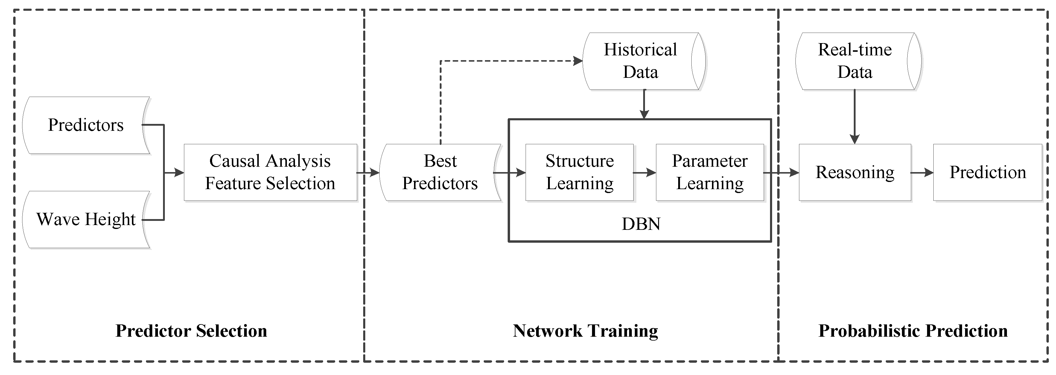
DBN and IF are combined to construct a probabilistic prediction model (DBN-IF). The model comprises three modules: predictor selection, DBN training, and probabilistic reasoning. First, the causal analysis between predictors and wave height is conducted by calculating IF to select best predictors. Then, DBN is constructed by structure learning and parameter learning on the basis of large historical data. Finally, the real-time data of predictors are input, and posterior probability distributions of wave height are obtained by probabilistic reasoning. Figure 1 summarizes the technique process and each module is elaborated as follows.

• Predictor Selection: calculate IF between predictors and wave height to identify their causal relationships, and select the variables having significant causality with wave height as the best predictors.
• Network Training: discretize the data of variables (predictors and wave height); mine causal relationships among variables based on historical data and adjust arcs according to professional knowledge, establishing the initial network and transition network; learn the conditional probability and the transition probability using intelligent algorithms.
• Probabilistic Prediction: discretize the real-time data of predictors and input them as prior evidence; calculate the posterior probability distributions of wave height in different time slices for probabilistic prediction.
• More technical details and implementation processes are explained in the next section.

3. Experiment and Analysis

In order to investigate the performance of the DBN-IF model in forecasting significant wave height, we carried out a number of experiments, in which measured data from moored ocean buoys were used. In the following prediction experiments, we present the data description, implementation details, and main results obtained with DBN-IF. Experiments were carried out with FULL-BNT v.1.0.4 Tool-Box (https://download.csdn.net/download/b08514/6942975).

3.1. Description of Data

The data obtained from buoys are a reliable data source due to less measurement errors and priori calibration. After combing the known studies, we preliminarily selected wind direction, wind speed, gust speed, dominant wave period, average wave period, direction of wave at dominant period, sea level pressure, air temperature, and sea surface temperature (a total of nine variables) as predictors. For the analysis and experiments, measured data of predictors and significant wave height (from 1 January to 31 December 2014) collected from buoys 51101 were used for model training and data (from 1 January to 31 December 2015) collected from buoys 41002 and 22103 were used for model testing (data source files from the web: https://www.ndbc.noaa.gov/).

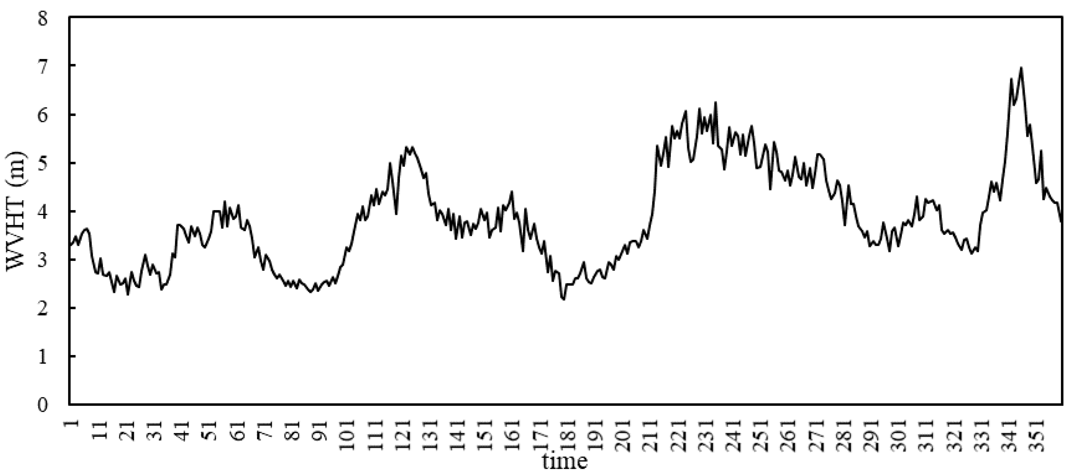
Take buoy 51101 as an example to analyze the data features of nine variables.

Table 1. Information and summary of measured data from buoy 51101.

Buoy: 51101	Depth: 4849 m (24.361° N, 162.075° W)
Variables	Maximum	Average	Minimum
Wind direction (WDIR, °)	360	117.947	1
Wind speed (WSPD, m/s)	15.4	6.908	0
Gust speed (GST, m/s)	20.4	8.506	0.2
Dominant wave period (DPD, s)	21.05	10.952	4.76
Average wave period (APD, s)	13.92	7.069	4.96
Direction of wave at dominant period (MVD, °)	360	173.408	1
Sea level pressure (PRES, Pa)	1026	1016.106	998.8
Air temperature (ATMP, ℃)	29.2	23.998	16.6
Sea surface temperature (WTMP, ℃)	30.2	25.082	20.8
Significant wave height (WVHT, m)	6.96	2.359	0.83

summarizes the buoy information and details of collected variables from buoy 51101 in 2014. It can be seen that there are relatively obvious differences about the statistical parameters of different variables. Some of the hourly times series records of significant wave height (WVHT) are presented in Figure 2. The nonlinearity and non-stationarity of WVHT time series are notable, which are barriers of accurate prediction.

3.2. Predictor Selection

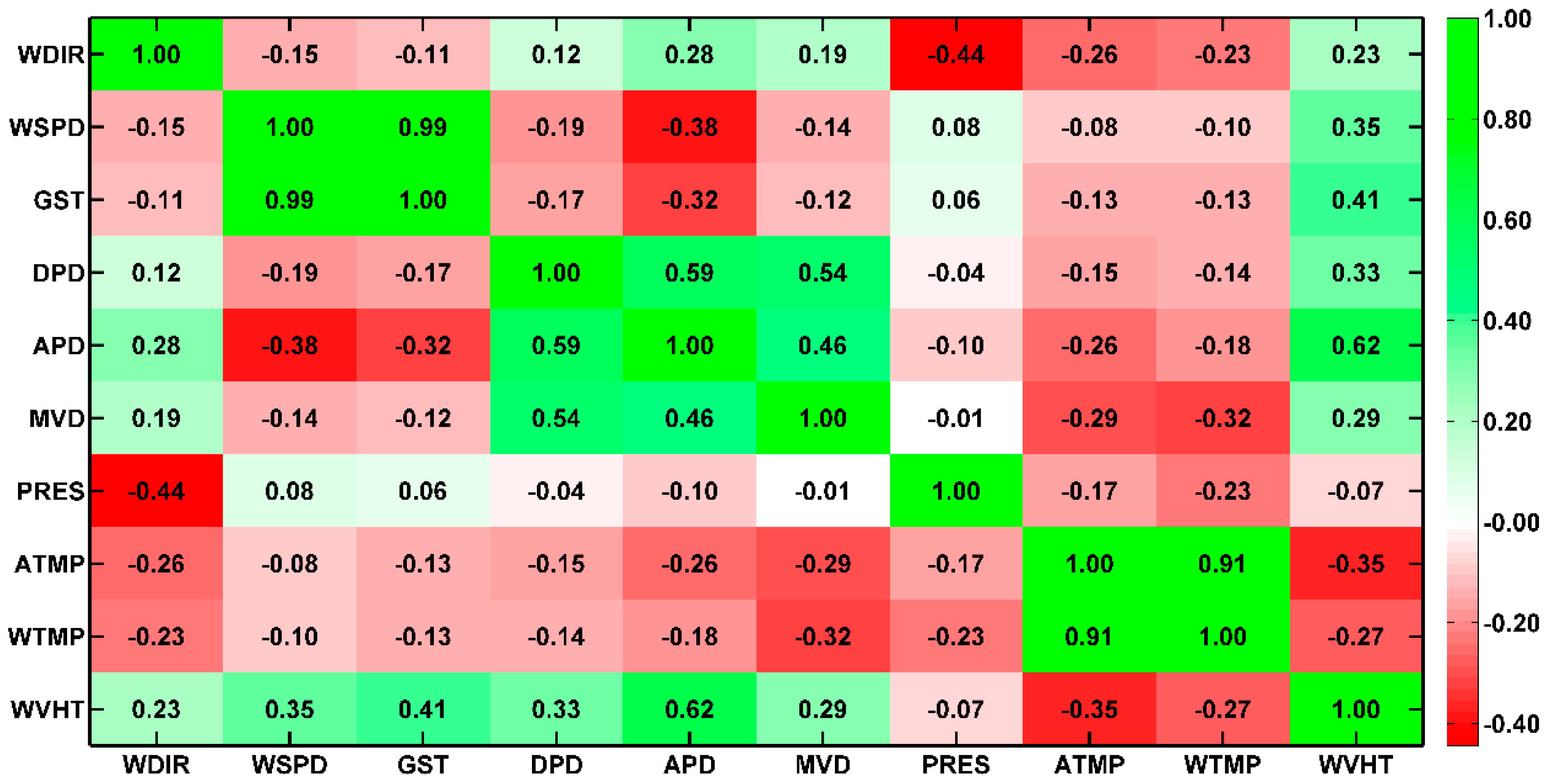
To investigate the validity of IF, correlation analysis was also conducted for predictor selection. Based on training data, we first calculated the correlation coefficient (CC) between different variables as shown in Figure 3. It can be summarized that (1) the correlations between predictors and WVHT vary greatly. It is necessary to reject poorly relative predictors. (2) The correlations between different predictors are also remarkable. Taking strongly relative predictors as input variables simultaneously could result in information redundancy, which increases the cost and running time of a prediction system, as well as degrades its generalization performance. Therefore, it is indispensable to select effective predictors.

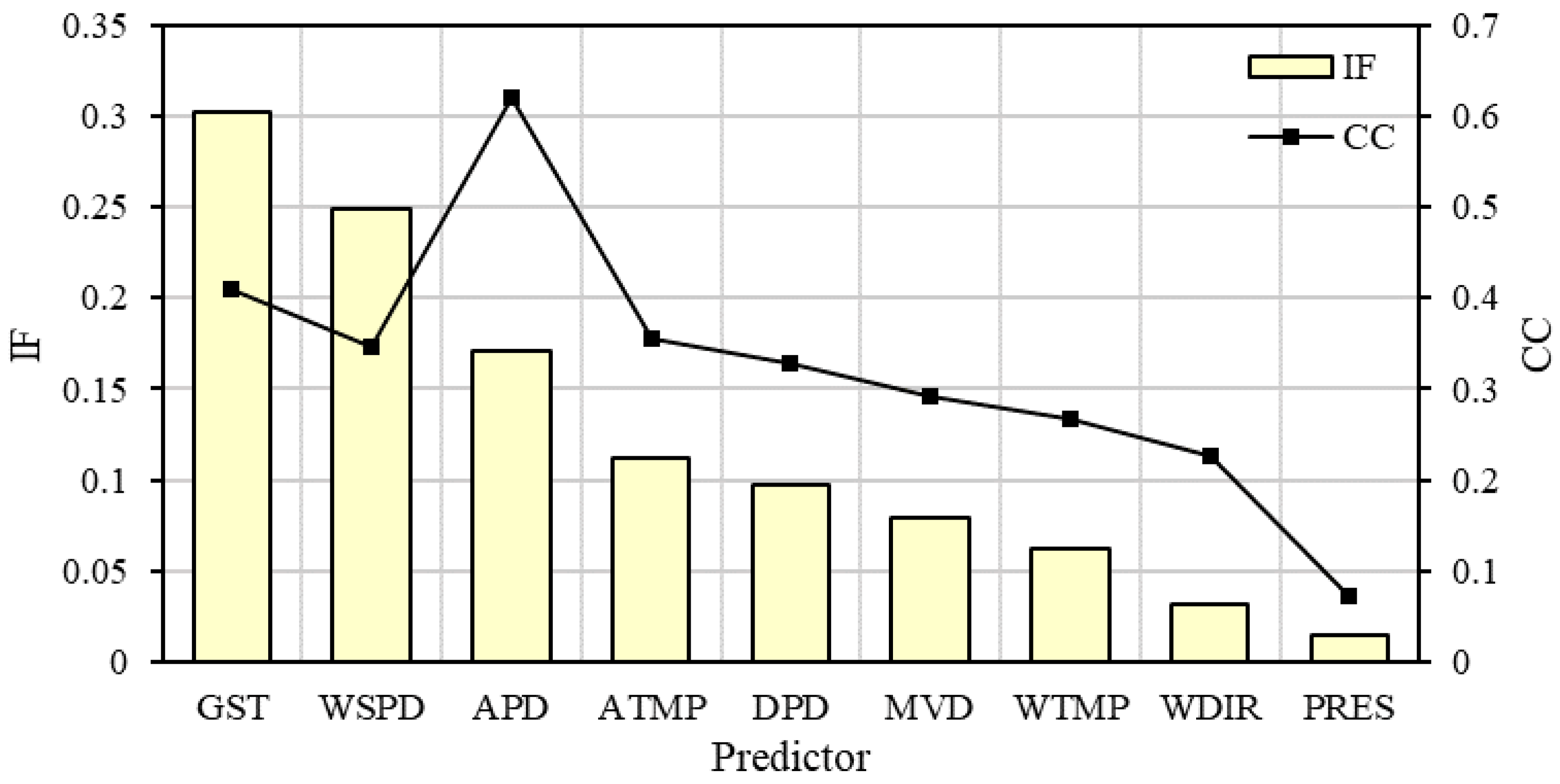
Correlation analysis shows the degree of relevance between predictors and WVHT; however, predictors closely related to WVHT are not necessarily the cause of WVHT on the basis of IF theory. Then we calculated the IF to compare with CC in

Table 2. Comparison of IF and CC. Statistically significant values at the 90% level are highlighted.

Variable		WDIR	WSPD	GST	DPD	APD	MVD	PRES	ATMP	WTMP
WVHT	IF	0.0323	0.2488	0.3025	0.0977	0.1707	0.0794	0.0146	0.1117	0.0622
	CC	0.2263	0.3472	0.4106	0.3287	0.6209	0.2928	−0.0726	−0.3543	−0.2677

, and Figure 4 presents the importance ranking of predictors in terms of both measures.

For IF, the predictors passing the significance test include GST, WSPD, APD, and ATMP. It is the biggest with IF of “GST→WVHT” and the next is “WSPD→WVHT”, which is in accord with the wind-wave generation mechanism. By contrast, for CC, the predictors passing the significance test include APD, GST, ATMP, WSPD, and DPD. It is the biggest with CC between APD and WVHT. Although APD is related to the growth of wave, it cannot be the cause of WVHT [34]. IF can identify the causal relationships. The best predictors selected by IF have better interpretability.

To further verify the reliability of IF, we respectively took the best predictors screened by IF and CC as input variables for nonlinear regression. The results are presented in

Table 3. Results of the nonlinear regression model.

The Best Predictors	Determinate Coefficient R2	F
IF: GST + WSPD + APD + ATMP	0.7934	4671.1564
CC: APD + GST + ATMP + WSPD + DPD	0.7061	2989.4381

.

Compared with “APD + GST + ATMP + WSPD + DPD”, the results obtained by “GST + WSPD +APD + ATMP” have bigger R² and F, indicating its regression equation is more significant. In this paper, we take “GST + WSPD + APD + ATMP” as best predictors.

3.3. DBN Training

The four predictors and WVHT were taken as DBN nodes. Then structure and parameter learning were carried out based on training data.

3.3.1. Data Discretization

As DBN is better at processing discrete data, the continuous data is required to be discretized to determine the number of states taken by nodes. We analyzed time series records over a period and selected reasonable interval division steps for variables. Then, variable states were denoted with consecutive numbers. Consequently, discrete data of each node were obtained with the equal interval division method. The discretization standard is shown in

Table 4. Discretization standard of variables.

Variables	WSPD	GST	APD	ATMP	WVHT
Interval step	0.5 m/s	0.5 m/s	0.5 s	0.5 ℃	0.5 m
State number	1–32	1–41	1–19	1–26	1–13

and

Table 5. Discrete training data.

Sample ID	WSPD	GST	APD	ATMP	WVHT
1	7	18	21	7	7
2	8	20	23	8	7
3	8	22	27	8	6
4	8	19	23	9	7
...	...	...	...	...	...
8721	3	4	4	7	8
8722	4	7	8	8	6

presents a part of the discrete training data.

3.3.2. Structure Learning

We adopted the advanced greedy search (AGS) method proposed in our published paper [35] to learn network structure, including the initial network structure and transition network structure. AGS comprises two steps: global causal analysis with IF and search for optimal structure with Greedy Search algorithm (GS).

Table 6. Algorithm scheme of AGS.

Input:	Training Data of Predictors and WVHT
Output:	Optimal DBN structure
Initialization:	Preprocess training data and set significant level
Causal analysis:	Calculate the IF between each two variables and analyze the causal relationships
Primitive structure:	Determine the arcs based on IF to obtain the primitive structure
Structure search:	Adopt GS algorithm to search for the optimal structure

shows the details of the AGS method.

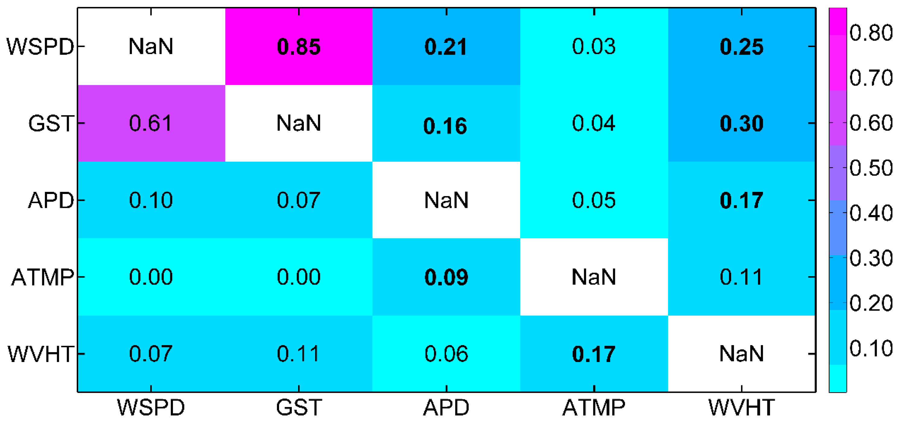
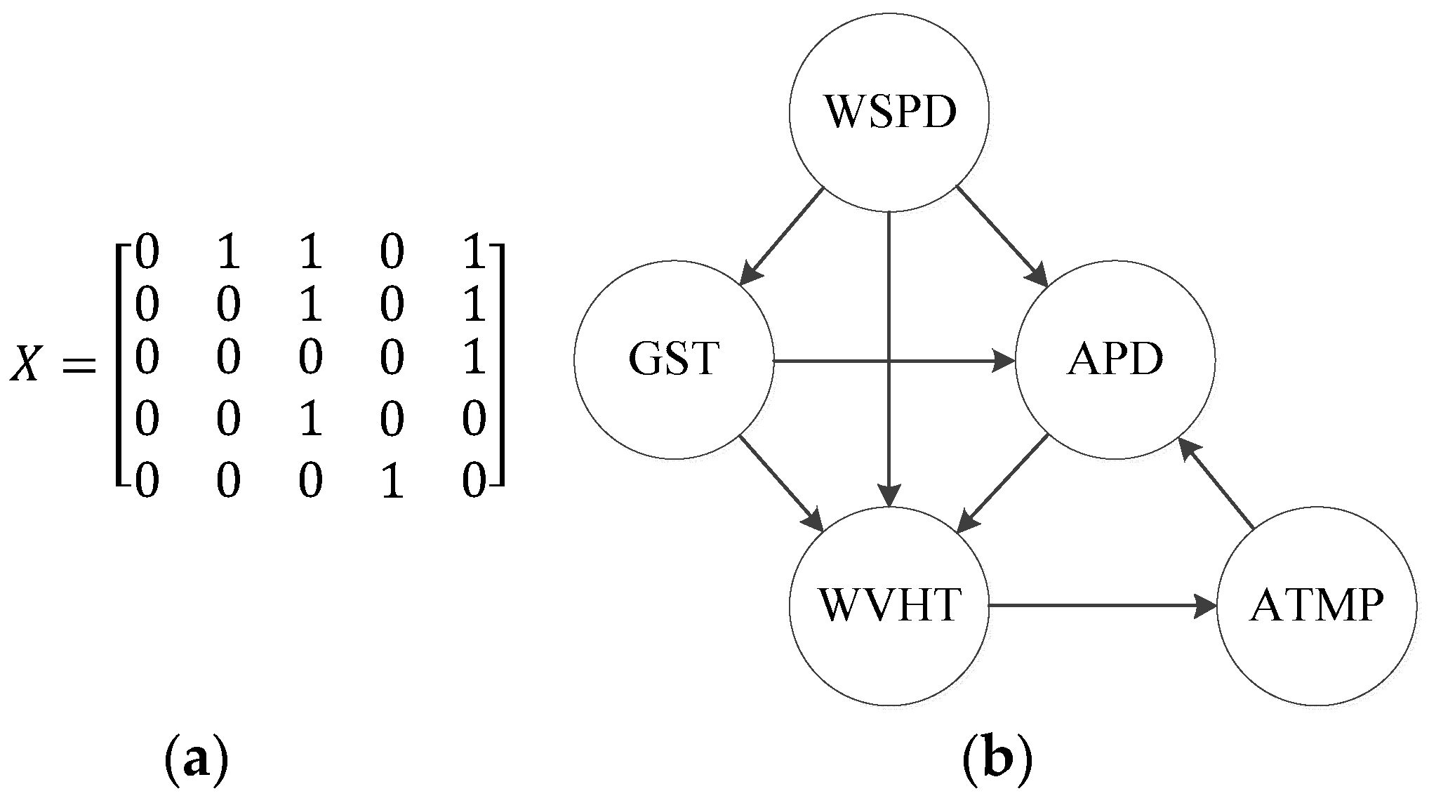
Step 1: Calculate IF between different variables and make a significant analysis of causal relationships. Figure 5 shows the result of causal analysis: as an example, $NI{F}_{\mathrm{WSPD}\to \mathrm{GST}}=0.8541$, $NI{F}_{\mathrm{GST}\to \mathrm{WSPD}}=0.6145$, both pass the significance test and $NI{F}_{\mathrm{WSPD}\to \mathrm{GST}}>NI{F}_{\mathrm{GST}\to \mathrm{WSPD}}$, so we could judge WSPD is the cause for GST. That is, there may be an arc “WSPD→GST” in the DBN. $NI{F}_{\mathrm{WSPD}\to \mathrm{ATMP}}=0.0337$, $NI{F}_{\mathrm{ATMP}\to \mathrm{WSPD}}=0.0021$, both do not pass the significance test so it is questionable to determine the arc between WSPD and ATMP. A preliminary analysis of the causal relationships is conducted to get the primitive structure. The adjacency matrix describing the relationship of WSPD, GST, APD, ATMP, and WVHT is shown in Figure 6a, and the corresponding primitive network structure is shown in Figure 6b.

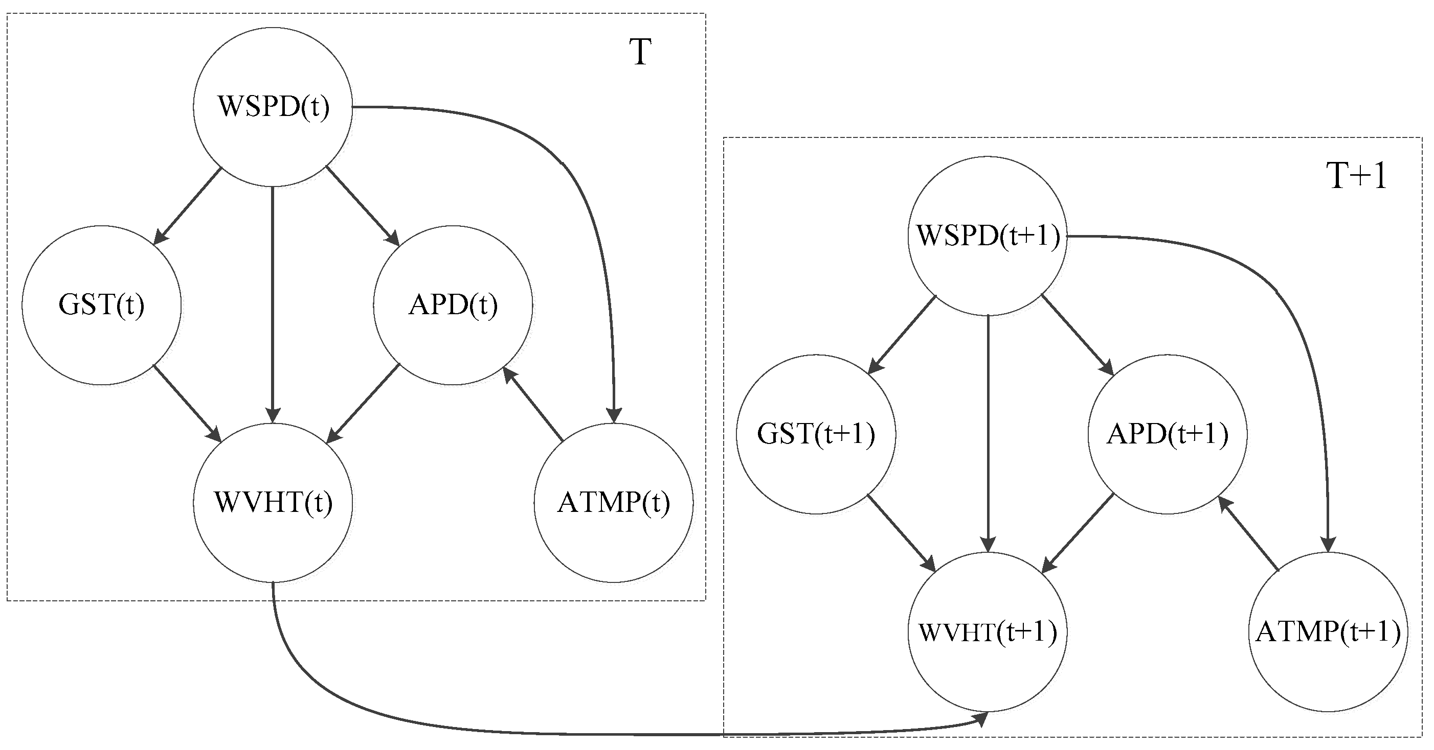
Step 2: Based on the discrete training data and the primitive structure, we adopt the GS algorithm to learn the initial network structure. Then connect the node WVHT of two adjacent time slices to build the transition network. Figure 7 visualizes the DBN structure, where the interactions of variables are expressed clearly. The initial network describes the causal relationship of WSPD, GST, APD, ATMP, and WVHT at time T. The transition network expresses the causal relationship of adjacent time (T to T + 1). DBN is better in interpretability, rather than a “Black Box”. Note that the time interval between two adjacent time slices is 1 h.

3.3.3. Parameter Learning

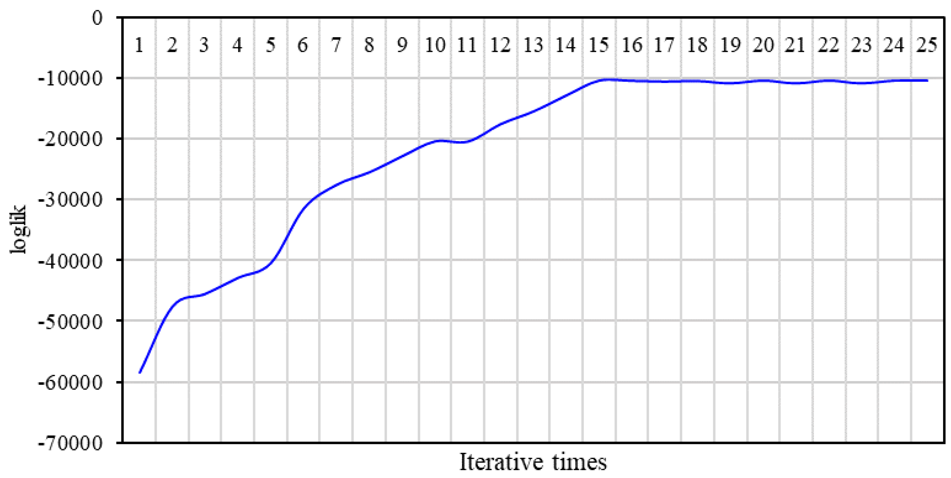
We adopted the expectation maximization (EM) algorithm for parameter learning. First, the probability distribution of each node was initialized, including prior probability, conditional probability, and transition probability. Then, based on the inference mechanism and training data, EM algorithm was used to modify the initial probability distribution, getting the probability distribution that matches the objective data.

Figure 8 shows that the result converges after 16 iterations. As an example, the transition probability distribution is shown in

Table 7. The transition probability distribution of node WVHT.

	(T + 1)	State of Node WVHT
(T)		1	2	3	4	5	6	7	8	9	10	11	12	13
State of node WVHT	1	0.774	0.226	0	0	0	0	0	0	0	0	0	0	0
	2	0.012	0.873	0.115	0	0	0	0	0	0	0	0	0	0
	3	0	0.056	0.855	0.089	0	0	0	0	0	0	0	0	0
	4	0	0	0.101	0.791	0.108	0.001	0	0	0	0	0	0	0
	5	0	0	0	0.203	0.663	0.132	0.002	0	0	0	0	0	0
	6	0	0	0	0.003	0.241	0.544	0.197	0.016	0	0	0	0	0
	7	0	0	0	0	0	0.264	0.536	0.172	0.024	0.004	0	0	0
	8	0	0	0	0	0	0.027	0.329	0.452	0.144	0.041	0.007	0	0
	9	0	0	0	0	0	0	0.036	0.298	0.440	0.202	0.024	0	0
	10	0	0	0	0	0	0	0	0.119	0.288	0.373	0.186	0.034	0
	11	0	0	0	0	0	0	0	0	0.097	0.290	0.387	0.129	0.097
	12	0	0	0	0	0	0	0	0	0	0.364	0.364	0.182	0.091
	13	0	0	0	0	0	0	0	0	0	0	0.167	0.500	0.333

. So far, the DBN-IF model for forecasting wave height is completed.

3.4. Results and Discussion

After training the model, WVHT time series were predicted using a part of testing data (from 1–16 February) collected from buoy 41002 (3920 m; 31.892° N, 74.930° W). Discrete data of predictors at current time were entered into DBN for probabilistic reasoning and predict WVHT in different lead times (1, 3, 6, 12, and 24 h).

Table A1. The posterior probability distributions of WVHT. The boldface font indicates the maximal probability.

	Time	Time Slices
State		1	2	3	4	5	6	7	8	9	10
State of Node WVHT	1	0	0	0	0	0	0	0	0	0	0
	2	0	0	0	2.27 × 10−25	6.89 × 10−21	2.00 × 10−21	0	1.83 × 10−21	8.49 × 10−22	0
	3	0	0	2.10 × 10−15	2.84 × 10−13	7.23 × 10−13	4.16 × 10−11	9.81 × 10−13	3.89 × 10−13	2.52 × 10−12	7.36 × 10−11
	4	0	3.24 × 10−10	9.62 × 10−08	3.54 × 10−08	2.43 × 10−08	5.68 × 10−08	5.77 × 10−08	7.12 × 10−09	8.05 × 10−08	1.41 × 10−07
	5	0	4.59 × 10−05	2.75 × 10−05	2.66 × 10−05	1.06 × 10−05	2.70 × 10−06	3.17 × 10−06	7.63 × 10−06	6.06 × 10−06	7.43 × 10−06
	6	0.033	0.00582	0.001888	0.000699	0.000469	0.000305	0.000321	0.000459	0.000355	0.000522
	7	0.180059	0.157232	0.009649	0.0049	0.005205	0.005988	0.00946	0.011799	0.011033	0.01301
	8	0.402809	0.512611	0.231684	0.171305	0.208138	0.485044	0.3264	0.131721	0.176065	0.656672
	9	0.379515	0.298365	0.617647	0.543321	0.611694	0.187613	0.389711	0.758889	0.695046	0.133887
	10	0.004616	0.025927	0.136526	0.272912	0.174483	0.299568	0.222023	0.097124	0.117495	0.195903
	11	0	0	0.002578	0.006837	0	0.021479	0.052082	0	0	0
	12	0	0	0	0	0	0	0	0	0	0
	13	0	0	0	0	0	0	0	0	0	0

presents the detailed posterior probability distributions of WVHT. The probabilistic predictions are able to express the probability of each state of WVHT in the next moment completely, dealing with the uncertainty of prediction.

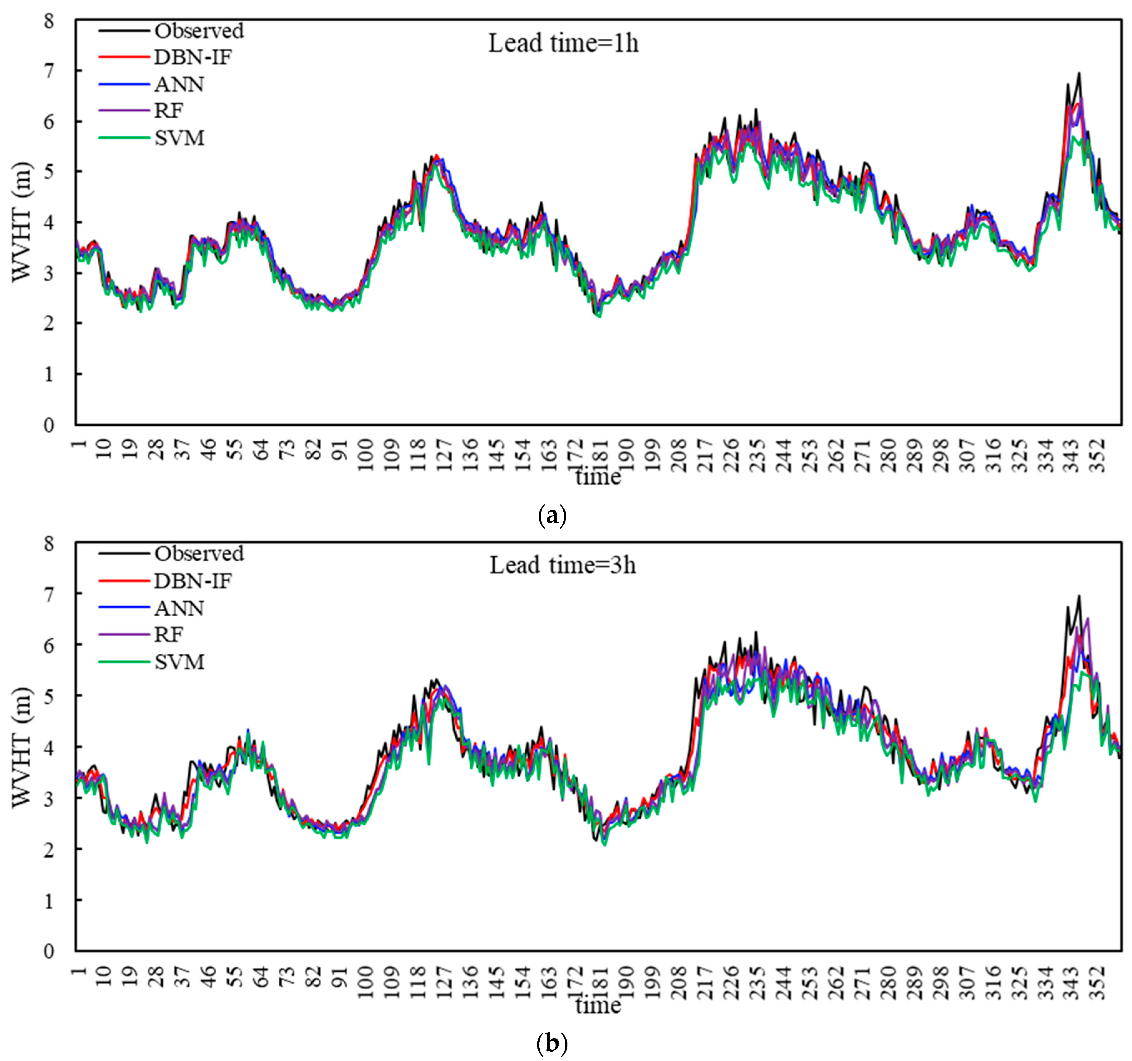
According to posterior probability distribution, we took the median in the most probable interval as the predictand of WVHT. In order to validate the performance of the DBN-IF, comparative investigations among ANN, RF, and SVM were conducted. Figure 9 presents the measured and predicted WVHT computed by different methods during the analysis period (from 1–16 February 2015).

As shown in Figure 9, all models show lower accuracy with increasing lead time. The peaks and troughs are well predicted by four models when the lead time is short (1, 3, and 6 h). By increasing the lead time (12 and 24 h), the differences, obtained from ANN, RF, and SVM, between the measured and predicted WVHT are obvious. However, the general patterns of the variations of WVHT are still reasonably captured by the DBN-IF model.

In addition, when the lead time reaches 12 and 24 h, shifts between the measured and predicted WVHT time series by ANN, RF, and SVM can be easily noted. It is easily found that the shifts obviously increase as the lead time grows. However, the shifts are overcome with DBN-IF because the transition network in DBN could achieve the real-time correction of errors to guarantee the accumulation of effective information. Predictands for the nonlinear and non-stationary WVHT are improved by combining IF with DBN.

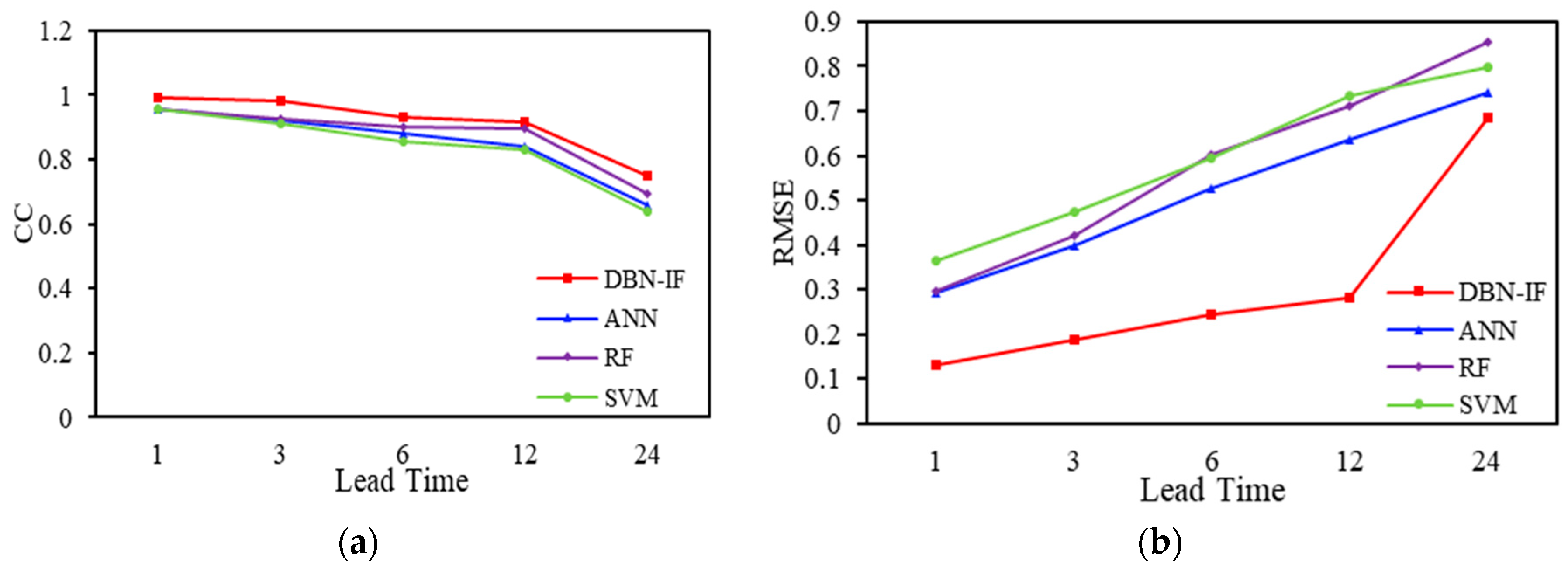
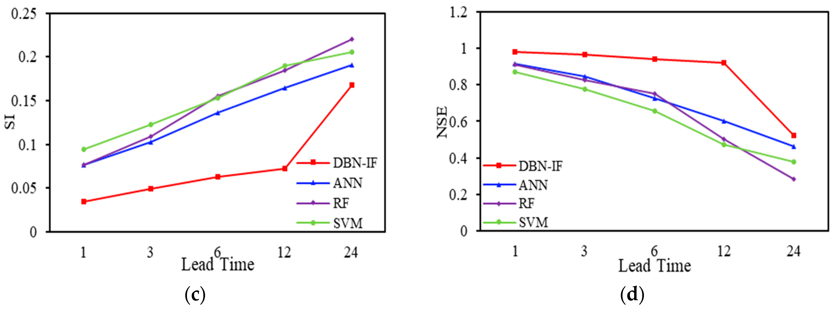
To investigate the performances for the above prediction models quantitatively, different error measures including the CC, root mean square error (RMSE), scatter index (SI), and Nash–Sutcliffe (NSE) were employed as evaluation criteria. We do not repeat CC and RMSE in consideration of space. SI and NSE as shown in Equations (6) and (7) are explained as follows.

$$\mathrm{SI}=\frac{\mathrm{RMSE}}{h_m}$$

(6)

$$\mathrm{NSE}=1-\frac{{{\displaystyle \sum }}_{i=1}^n{\left(\widehat{h_i}-h_i\right)}^2}{{{\displaystyle \sum }}_{i=1}^n{\left(h_i-h_m\right)}^2}$$

(7)

where $\widehat{h_i}$ is the predicted results, $h_i$ is the measured WVHT, $h_m$ is the mean value of $h_i$, and $n$ represents the length of test time series. The RMSE is a good measure for evaluating the performance of a model because RMSE is proportional to the observed mean. Therefore, the SI forms a good non-dimensional error measure. NSE compares the goodness of fit between the observed and predicted data. A high value of NSE (up to one) indicates high efficiency of the model [15].

Details of the CC, RMSE, SI, and NSE of WVHT predictions at the studied buoy 41002 are summarized in

Table 8. The CC, root mean square error (RMSE), scatter index (SI), Nash–Sutcliffe (NSE) of WVHT predictions with lead time = 1 h.

Criteria	DBN-IF	ANN	RF	SVM
CC	0.9927	0.9569	0.9585	0.9587
RMSE	0.1318	0.2948	0.2974	0.3641
SI	0.0341	0.0762	0.0769	0.0941
NSE	0.9829	0.9149	0.9134	0.8703

,

Table 9. The CC, RMSE, SI, NSE of WVHT predictions with lead time = 3 h.

Criteria	DBN-IF	ANN	RF	SVM
CC	0.9839	0.9223	0.9251	0.9102
RMSE	0.1895	0.3987	0.4203	0.4759
SI	0.0491	0.1031	0.1087	0.1231
NSE	0.9648	0.8444	0.8272	0.7784

,

Table 10. The CC, RMSE, SI, NSE of WVHT predictions with lead time = 6 h.

Criteria	DBN-IF	ANN	RF	SVM
CC	0.9334	0.8815	0.9024	0.8562
RMSE	0.2428	0.5272	0.6024	0.5935
SI	0.0628	0.1363	0.1557	0.1534
NSE	0.9423	0.7281	0.7524	0.6553

,

Table 11. The CC, RMSE, SI, NSE of WVHT predictions with lead time = 12 h.

Criteria	DBN-IF	ANN	RF	SVM
CC	0.9142	0.8423	0.8981	0.8284
RMSE	0.2814	0.6356	0.7132	0.7346
SI	0.0727	0.1643	0.1844	0.1899
NSE	0.9225	0.6047	0.5023	0.4721

and

Table 12. The CC, RMSE, SI, NSE of WVHT predictions with lead time = 24 h.

Criteria	DBN-IF	ANN	RF	SVM
CC	0.7523	0.6601	0.6932	0.6392
RMSE	0.6856	0.7427	0.8541	0.7965
SI	0.1676	0.1913	0.2208	0.2059
NSE	0.5248	0.4641	0.2862	0.3792

. Details of the error measures are plotted in Figure 10 to show the relations between their magnitudes and the prediction lead times.

When lead time = 1 h, for all models, the CC is greater than 0.95, RMSE is lower than 0.4, and SI is lower than 0.1. The performances of four models are similar, and DBN-IF is slightly better than the other three models. When lead time reaches 3 h, error measures of DBN-IF change little, but the other three models change a great deal. The NSE of ANN, RF, and SVM decline to about 0.8. By increasing lead time (6 and 12 h), the forecasting accuracy of DBN-IF remains high (CC > 0.9, RMSE < 0.3, SI < 0.1 and NSE > 0.9). The performances of the other three models are significantly lower than DBN-IF. Note that, when lead time reaches 12 h, the prediction accuracy of DBN-IF declines dramatically, although it is still the best.

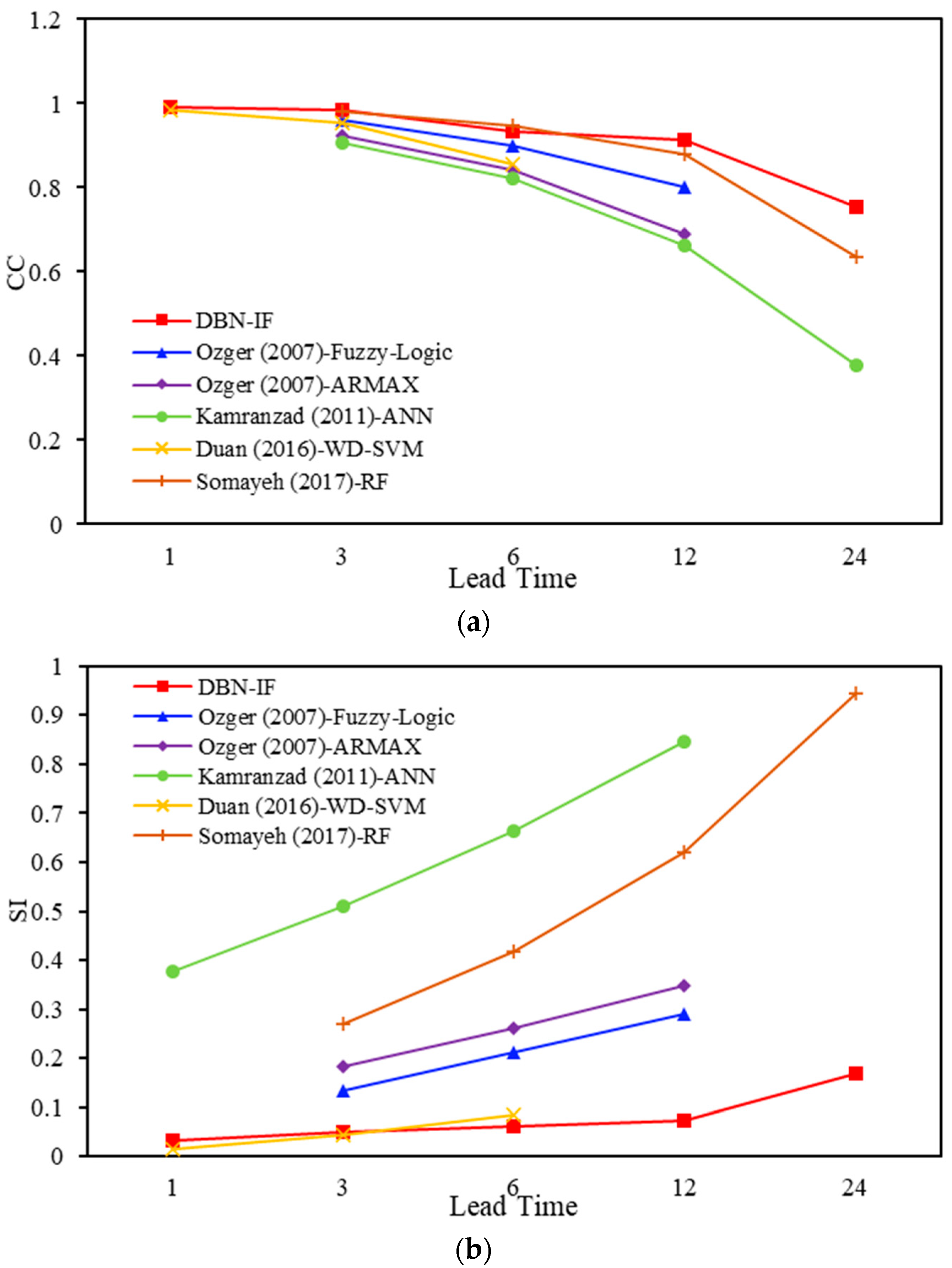
Previous studies used different input predictors to forecast WVHT. We re-achieved these models based on the same testing data (from 1 to 16 February buoy 41002).

Table 13. The predictions of different methods and different input predictors.

Reference	Lead Time	CC	SI	Model	Predictors
Ozger [12]	3 6 12	0.960 0.899 0.800	0.135 0.211 0.289	Fuzzy-Logic	Wind speed Significant wave height
Ozger [12]	3 6 12	0.925 0.842 0.690	0.184 0.260 0.349	ARMAX	Wind speed Significant wave height
Kamranzad [5]	3 6 12 24	0.907 0.820 0.663 0.379	0.378 0.511 0.663 0.845	ANN	Friction velocity Wind direction Significant wave height Wave direction
Duan [15]	1 3 6	0.986 0.954 0.855	0.014 0.044 0.086	WD-SVM	Significant wave height
Somayeh [16]	3 6 12 24	0.981 0.948 0.880 0.635	0.270 0.418 0.619 0.945	RF	Wind speed Significant wave height Wave period Pressure Air temperature Water temperature Dew point

summarizes the studies that applied different ML-based approaches and different input predictors to forecast WVHT in different lead times.

In comparison to Kamranzad [5] and Somayeh [16], it is easy to see that the predictor selection process affects the performance of the prediction model, improving its accuracy. When using ANN for prediction, the results with input predictors selected by IF are more accuracy markedly. When using RF, different input predictors have similar predictions with short lead times (3 and 6 h); however, when lead time reaches 12 and 24 h, the results with input predictors selected by IF are better. Furthermore, Figure 11 visualizes the comparison between different methods where the current study outperformed other studies and methods.

In order to complete this experiment section, we selected another buoy 22103 (130 m; (34.012° N, 127.503° W) and longer analysis period (from 1 January to 31 December 2015) for prediction experiments to test the generalization ability of the DBN-IF. Predictions of WVHT in different locations show consistent conclusions. Seen from

Table 14. The CC, RMSE, SI, NSE of WVHT predictions with lead time = 6 h.

Criteria	DBN-IF	ANN	RF	SVM
CC	0.9114	0.8672	0.8801	0.8542
RMSE	0.2165	0.3947	0.3851	0.4131
SI	0.1436	0.1758	0.1721	0.2164
NSE	0.9142	0.7561	0.7873	0.6983

and

Table 15. The CC, RMSE, SI, NSE of WVHT predictions with lead time = 12 h.

Criteria	DBN-IF	ANN	RF	SVM
CC	0.8792	0.8211	0.8536	0.8147
RMSE	0.3489	0.4361	0.4253	0.5326
SI	0.1735	0.2083	0.1969	0.2945
NSE	0.8803	0.7206	0.7367	0.6714

, DBN-IF outperforms ANN, RF, and SVM. In addition, compared with long-term prediction, the proposed model is better at short-term prediction.

4. Conclusion

In this paper, we introduced causal IF and DBN to propose a novel probabilistic prediction model (DBN-IF) for significant wave height. In this ML-based model, we first introduced IF theory to select the best predictors by analyzing the causal relationships between wave height and other meteorological and oceanographic variables. Then, we extracted and quantitatively expressed the interactions among variables by structure and parameter learning to construct the DBN. Finally, predictions of wave height were achieved by probabilistic reasoning. Experimental results show that the performance of the DBN-IF model in predicting the hourly wave height is superior to those of primary ML-based models (ANN, SVM, and RF). The high accuracy of the DBN-IF model is attributed to the following two prominent advantages:

• Emphasis on screening of predictors. Different from the previous prediction models, the first step of our proposed model is to analyze and screen predictors. Use state-of-the-art IF theory instead of correlation coefficient or time-delay correlation coefficient to perform causal analysis between predictors and wave height to select the best predictors;
• Good interpretability of prediction model and ability to deal with uncertainty. Based on graph theory and probability theory, DBN can not only visualize the relationships among predictive variables but also quantitatively express the interactions with probability distributions. On the one hand, it handles the “Black Box” problem that ML algorithms such as ANN, SVM, and RF are difficult to explain. On the other hand, it deals with the uncertainty of nonlinear wave height time series through probability theory.

However, the DBN-IF model requires a large amount of data for training, so the application is limited in locations without wave buoys. Additionally, it does not perform well in long-term prediction. The future work scope involves information redundancy in predictor selection, long-term prediction of wave height, and also DBN-based prediction models with no need for much data. This work shall be extended to other major offshore activity regions across the world to enable support in offshore operation and marine control applications.

References

- Zheng, C.W.; Li, C.Y. Variation of the wave energy and significant wave height in the China sea and adjacent waters. Renew. Sustain. Energy Rev. 2015, 43, 381–387. [Google Scholar] [CrossRef]
- Zheng, C.W.; Wu, G.X.; Chen, X. CMIP5-based wave energy projection: Case studies of the South China Sea and the East China Sea. IEEE Access 2019, 31, 329–337. [Google Scholar] [CrossRef]
- Janssen, P. Progress in ocean wave forecasting. J. Comput. Phys. 2008, 227, 3572–3594. [Google Scholar] [CrossRef]
- Goda, Y. Revisiting Wilson’s formulas for simplified wind-wave prediction. J. Waterw. Port Coast. Ocean Eng. 2003, 129, 93–95. [Google Scholar] [CrossRef]
- Kamranzad, B.; Etemad-Shahidi, A.; Kazeminezhad, M.H. Wave height forecasting in Dayyer, the Persian Gulf. Ocean Eng. 2011, 38, 248–255. [Google Scholar] [CrossRef] [Green Version]
- Spanos, P. ARMA algorithms for ocean wave modeling. J. Energy Resour. Technol. 1983, 105, 300–309. [Google Scholar] [CrossRef]
- Altunkaynak, A.; Özger, M. Temporal significant wave height estimation from wind speed by perceptron Kalman filtering. Ocean Eng. 2004, 31, 1245–1255. [Google Scholar] [CrossRef]
- Valipour, M.; Banihabib, M.E.; Behbahani, S.M.R. Comparison of the ARMA, ARIMA, and the autoregressive artificial neural network models in forecasting the monthly inflow of Dez dam reservoir. J. Hydrol. 2013, 476, 433–441. [Google Scholar] [CrossRef]
- Stefanakos, C. Fuzzy time series forecasting of nonstationary wind and wave data. Ocean Eng. 2016, 121, 1–12. [Google Scholar] [CrossRef] [Green Version]
- Deo, M.C.; Naidu, C.S. Real time forecasting using neural networks. Ocean Eng. 1998, 26, 191–203. [Google Scholar] [CrossRef]
- Lee, T.L. Neural network prediction of a storm surge. Ocean Eng. 2006, 33, 483–494. [Google Scholar] [CrossRef]
- Ozger, M. Significant wave height forecasting using wavelet fuzzy logic approach. Ocean Eng. 2010, 37, 1443–1451. [Google Scholar] [CrossRef]
- Shahabi, S.; Khanjani, M.J.; Kermani, M.R.H. Significant wave height modelling using a hybrid wavelet-genetic programming approach. KSCE J. Civil Eng. 2017, 21, 1–10. [Google Scholar] [CrossRef]
- Mahjoobi, J.; Mosabbeb, E.A. Prediction of significant wave height using regressive support vector machines. Ocean Eng. 2009, 36, 339–347. [Google Scholar] [CrossRef]
- Duan, W.Y.; Han, Y.; Huang, L.M.; Zhao, B.B.; Wang, M.H. A hybrid EMD-SVR model for the short-term prediction of significant wave height. Ocean Eng. 2016, 124, 54–73. [Google Scholar] [CrossRef]
- Mafi, S.; Amirinia, G. Forecasting hurricane wave height in Gulf of Mexico using soft computing methods. Ocean Eng. 2017, 146, 352–362. [Google Scholar] [CrossRef]
- Hatalis, K. Multi-step forecasting of wave power using a nonlinear recurrent neural network. In Proceedings of the IEEE Pes General Meeting, National Harbor, MD, USA, 27–31 July 2014. [Google Scholar]
- Gasse, M.; Millioz, F.; Roux, E.; Garcia, D.; Liebgott, H.; Friboulet, D. High-quality plane wave compounding using convolutional neural networks. IEEE Trans. Ultrason. Ferroelectr. Freq. Control 2017, 64, 1637–1639. [Google Scholar] [CrossRef] [Green Version]
- Cornejo-Bueno, L.; Nieto-Borge, J.C.; García-Díaz, P.; Rodríguez, G.; Salcedo-Sanz, S. Significant wave height and energy flux prediction for marine energy applications: A grouping genetic algorithm—Extreme learning machine approach. Renew. Energy 2016, 97, 380–389. [Google Scholar] [CrossRef]
- Weston, J.; Mukherjee, S.; Chapelle, O.; Pontil, M.; Vapnik, V. Feature selection for SVMs. Adv. Neural Inf. Process. Syst. 2000, 11, 526–532. [Google Scholar]
- Blum, A.L.; Langrey, P. Selection of relevant features and examples in machine learning. Artif. Intell. 1997, 97, 245–271. [Google Scholar] [CrossRef] [Green Version]
- Salcedo-Sanz, S.; Prado-Cumplido, M.D.; Pérez-Cruz, F.; Bousoño-Calzón, C. Feature selection via genetic optimization. In International Conference on Artificial Neural Networks; Springer: Berlin/Heidelberg, Germany, 2002; pp. 547–552. [Google Scholar]
- Landman, W.A.; Mason, S.J. Forecasts of near-global sea surface temperatures using canonical correlation analysis. J. Clim. 2001, 14, 3819–3833. [Google Scholar] [CrossRef]
- Juneng, L.; Tangang, F.T. Level and source of predictability of seasonal rainfall anomalies in Malaysia using canonical correlation analysis. Int. J. Climatol. 2008, 28, 1255–1267. [Google Scholar] [CrossRef]
- San Liang, X. Unraveling the cause-effect relation between time series. Phys. Rev. E 2014, 90, 052150. [Google Scholar] [CrossRef] [Green Version]
- Li, M.; Liu, K.F. Causality-based attribute weighting via information flow and genetic algorithm for naive bayes classifier. IEEE Access 2019, 7, 150630–150641. [Google Scholar] [CrossRef]
- Schaefer, H. Entering the black box of neural networks. Methods Inf. Med. 2003, 42, 287–296. [Google Scholar]
- Liang, S.X. Normalizing the causality between time series. Phys. Rev. E 2015, 92, 022126. [Google Scholar] [CrossRef] [Green Version]
- Sun, J.; Sun, J. A dynamic Bayesian network model for real-time crash prediction using traffic speed conditions data. Transp. Res. Part C Emerging Technol. 2015, 54, 176–186. [Google Scholar] [CrossRef]
- Xiao, Q.; Chaoqin, C.; Li, Z. Time series prediction using dynamic Bayesian network. Optik 2017, 135, 98–103. [Google Scholar] [CrossRef]
- Li, M.; Liu, K.F. Application of intelligent dynamic Bayesian network with wavelet analysis for probabilistic prediction of storm track intensity index. Atmosphere 2018, 9, 224. [Google Scholar] [CrossRef] [Green Version]
- Pearl, J. From Bayesian networks to causal networks. In Mathematical Models for Handling Partial Knowledge in Artificial Intelligence; Springer: Berlin, Germany, 1995; pp. 157–182. [Google Scholar]
- Cussens, J. Bayesian network learning with cutting planes. arXiv 2012, arXiv:1202.3713v1. Available online: https://arxiv.org/abs/1202.3713 (accessed on 3 June 2012).
- Mao, J.Y.; Xie, H.R. Review of Wind-Wave Generation Mechanisms. Adv. Mar. Sci. 2019, 37, 533–542. [Google Scholar]
- Li, M.; Zhang, R.; Hong, M.; Bai, C. Improved structural learning algorithm of Bayesian network based on information flow. Syst. Eng. Electron. 2018, 465, 202–207. [Google Scholar]
Figure 1.
Technical flowchart of dynamic Bayesian network and information flow (DBN-IF model).
Figure 2.
Time series records of WVHT in buoy 51101.
Figure 3.
Correlation coefficients (CCs) between different variables.
Figure 4.
Importance ranking of predictors.
Figure 5.
IF between different variables.
Figure 6.
Results of causal analysis; (a) adjacency matrix, (b) primitive structure.
Figure 7.
DBN structure of WVHT prediction.
Figure 8.
Iterative curve of expectation maximization (EM) algorithm.
Figure 9.
Observed and predicted WVHT during the study period with four methods and different lead times: (a) 1 h, (b) 3 h, (c) 6 h, (d) 12 h, (e) 24 h.
Figure 10.
Error measures with four methods and different lead time: (a) CC, (b) RMSE, (c) SI, (d) NSE.
Figure 11.
The CC and SI of different methods: (a) CC, (b) SI