Spatial Predictions of Debris Flow Susceptibility Mapping Using Convolutional Neural Networks in Jilin Province, China

 ,
,
Abstract
:1. Introduction
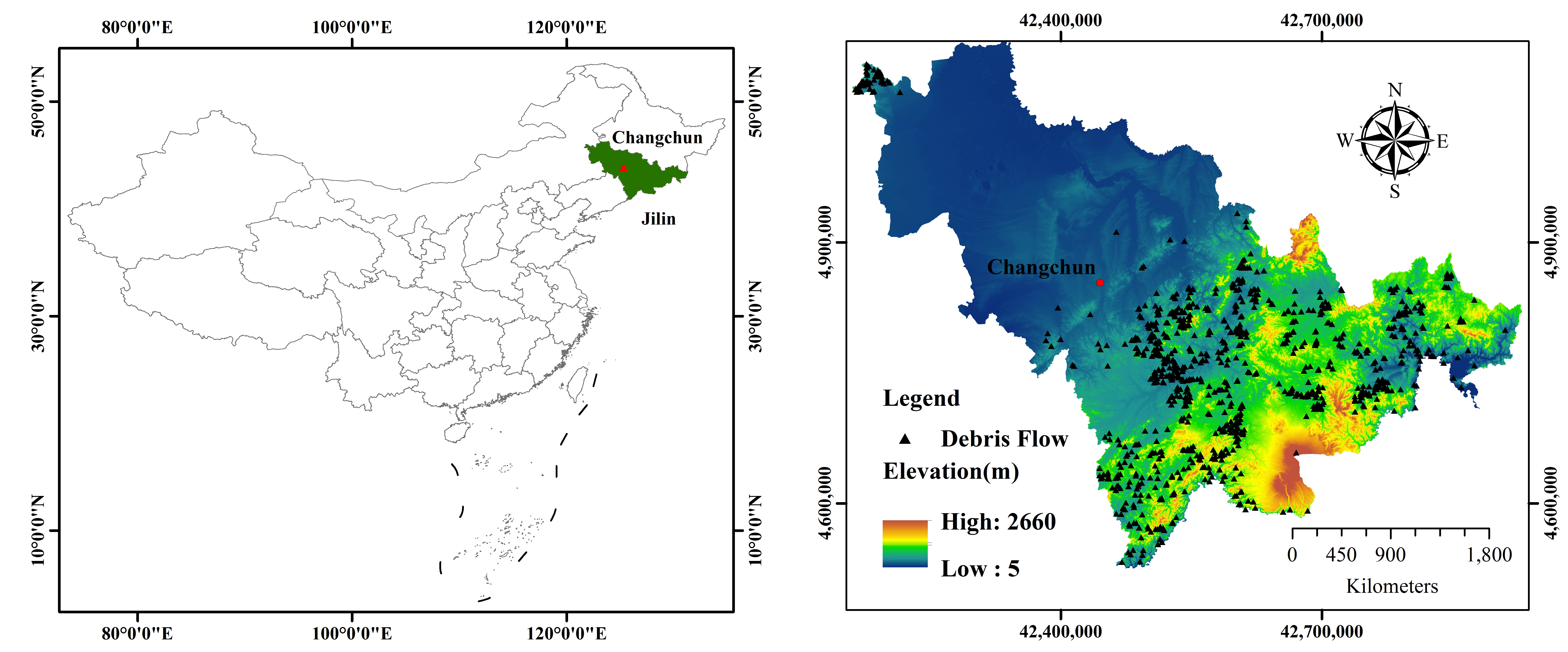
2. Study Area
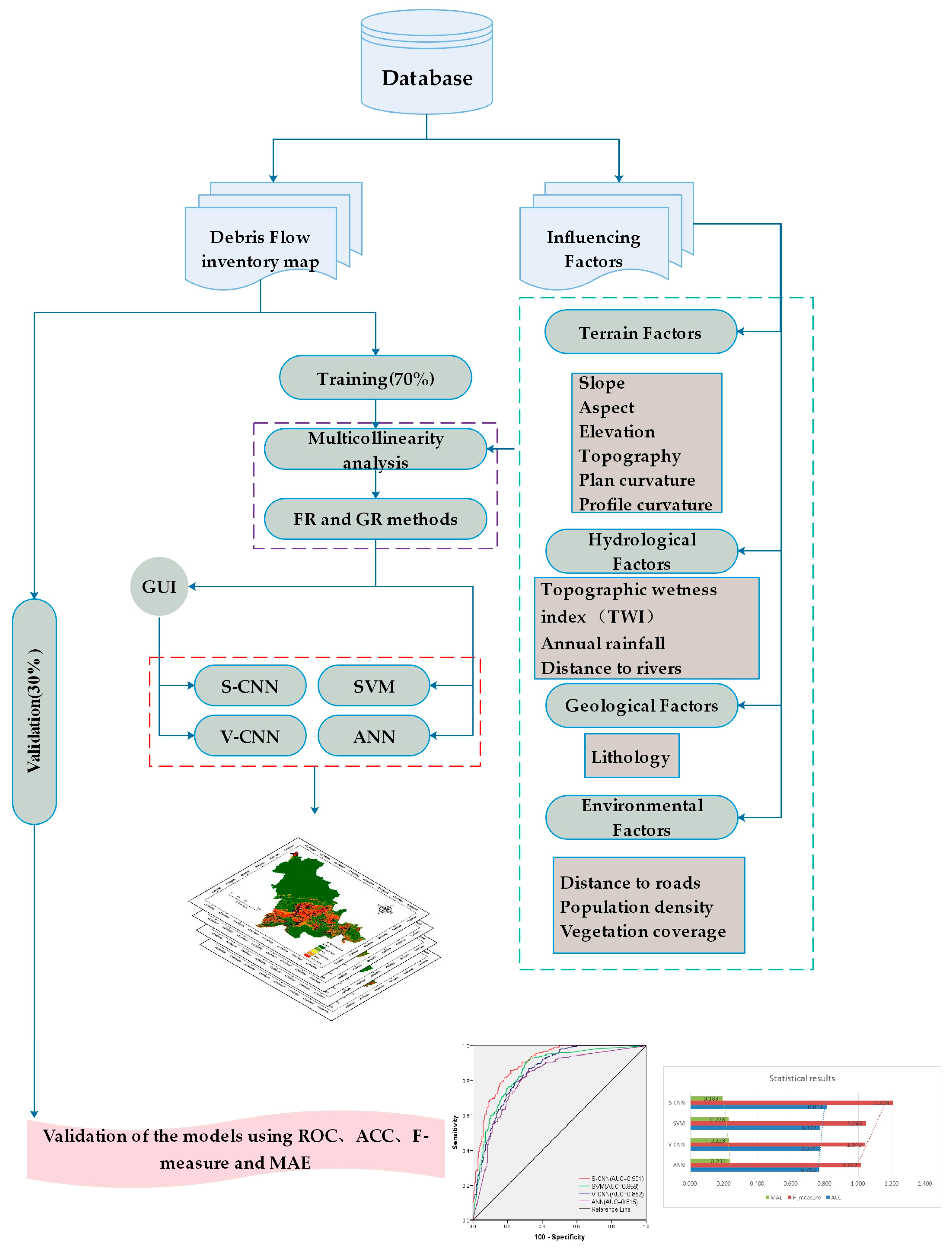
3. Materials and Methods
3.1. Data Preparation
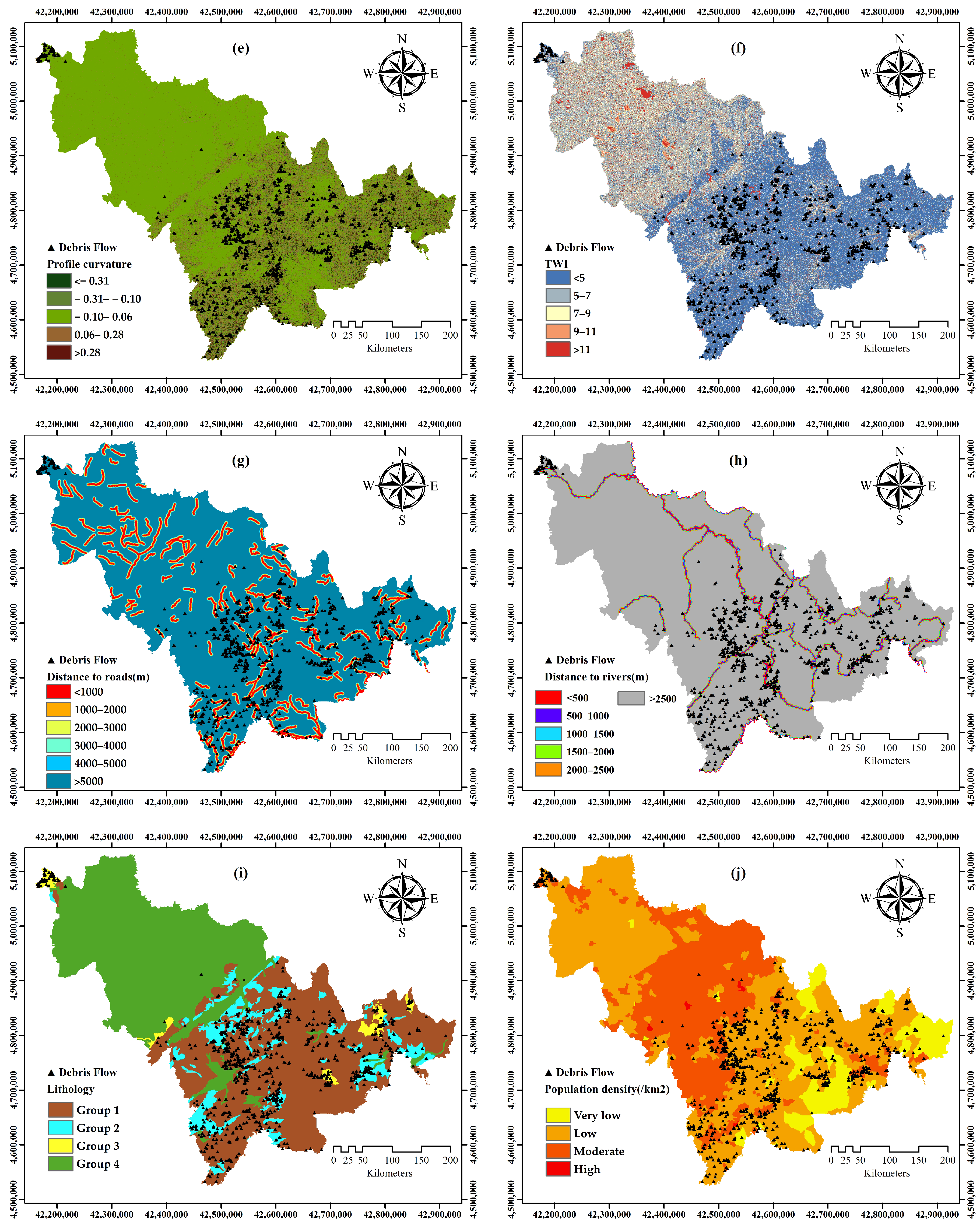
3.2. Influencing Factors
3.3. Evaluation of Influencing Factors
3.3.1. Multicollinearity Analysis
3.3.2. Frequency Ratio Method
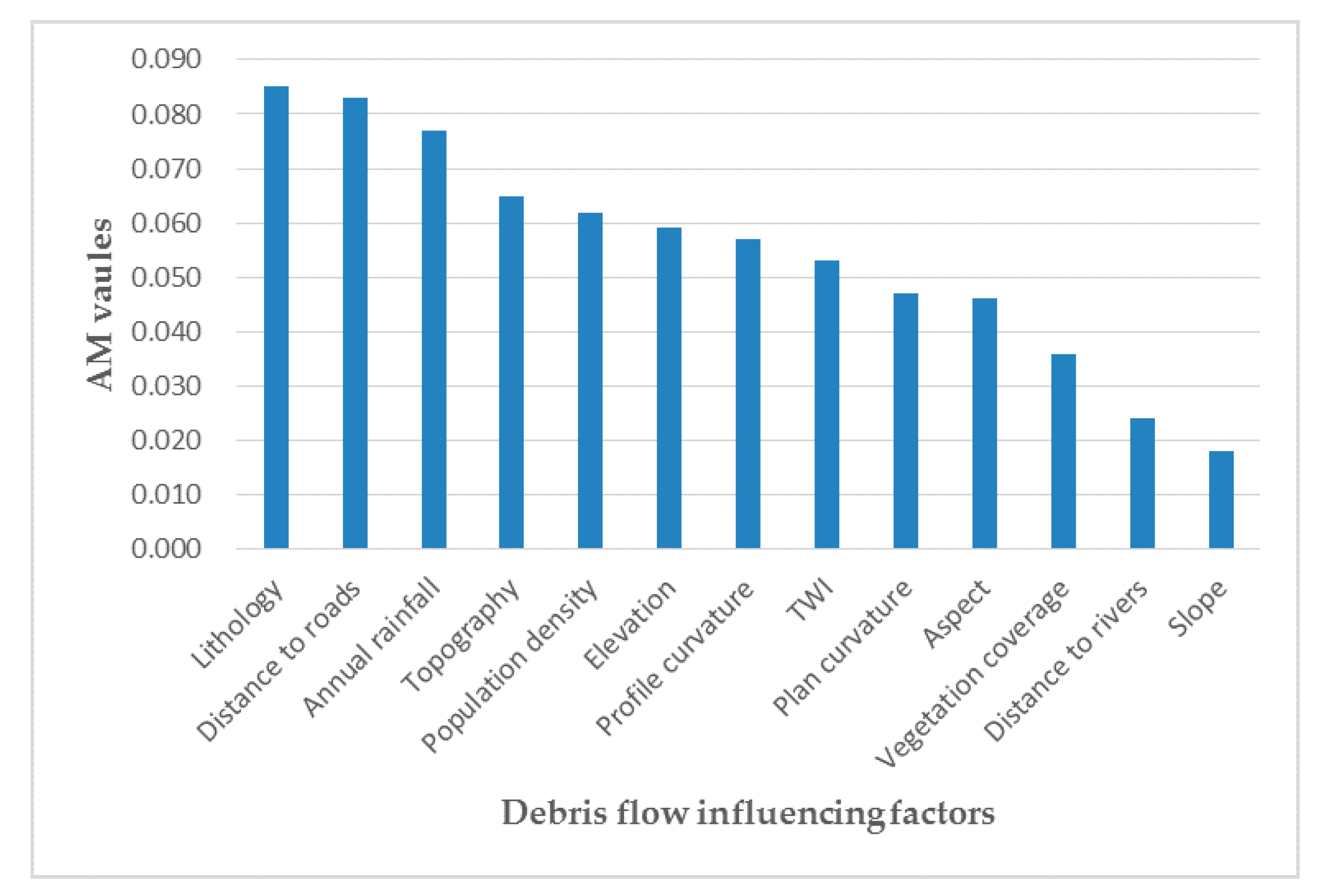
3.3.3. Gain Ratio Method
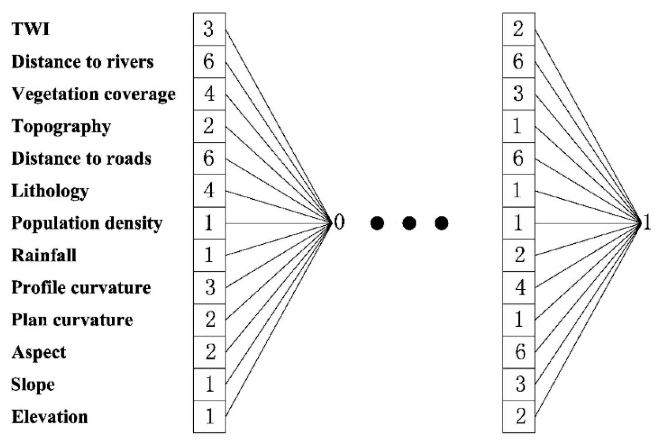
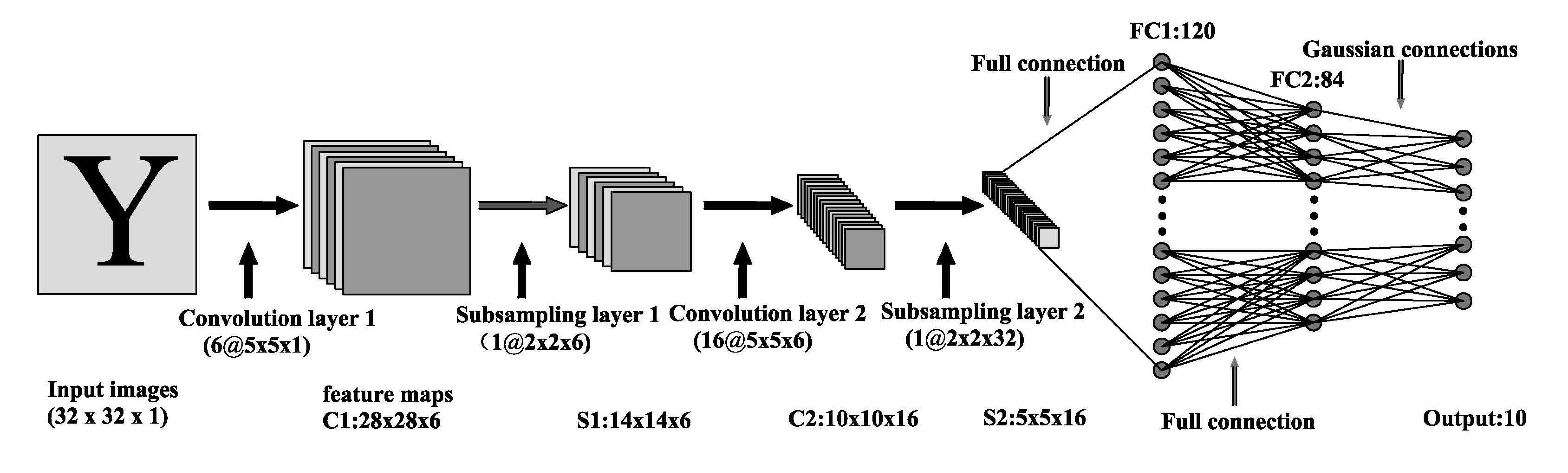
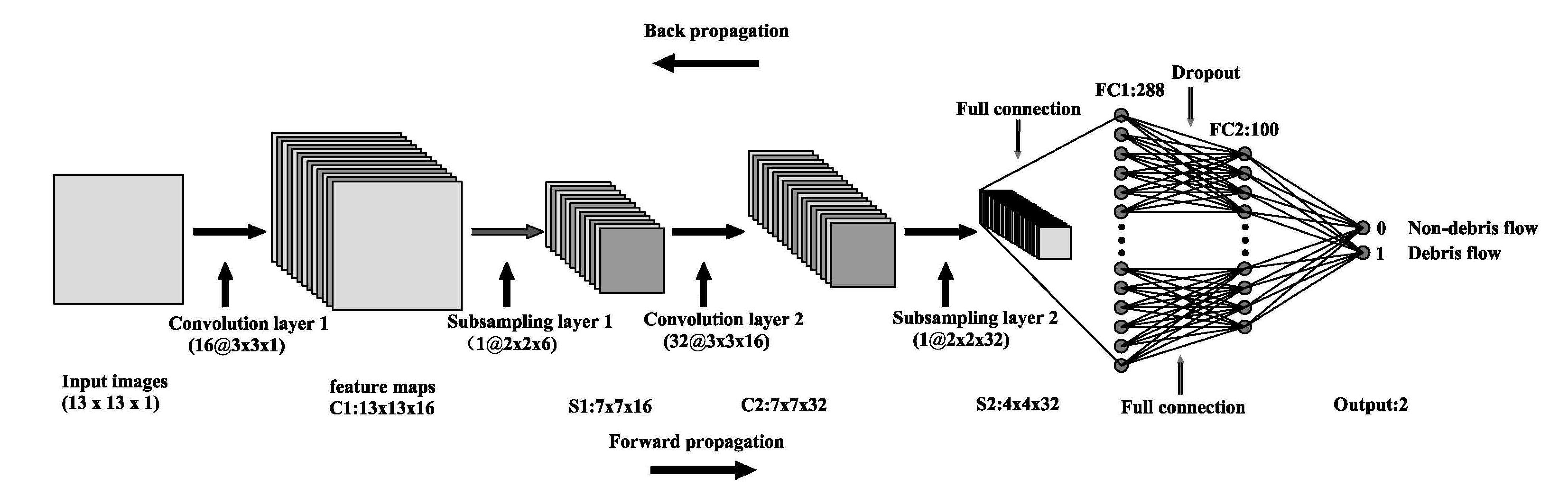
3.4. V–CNN
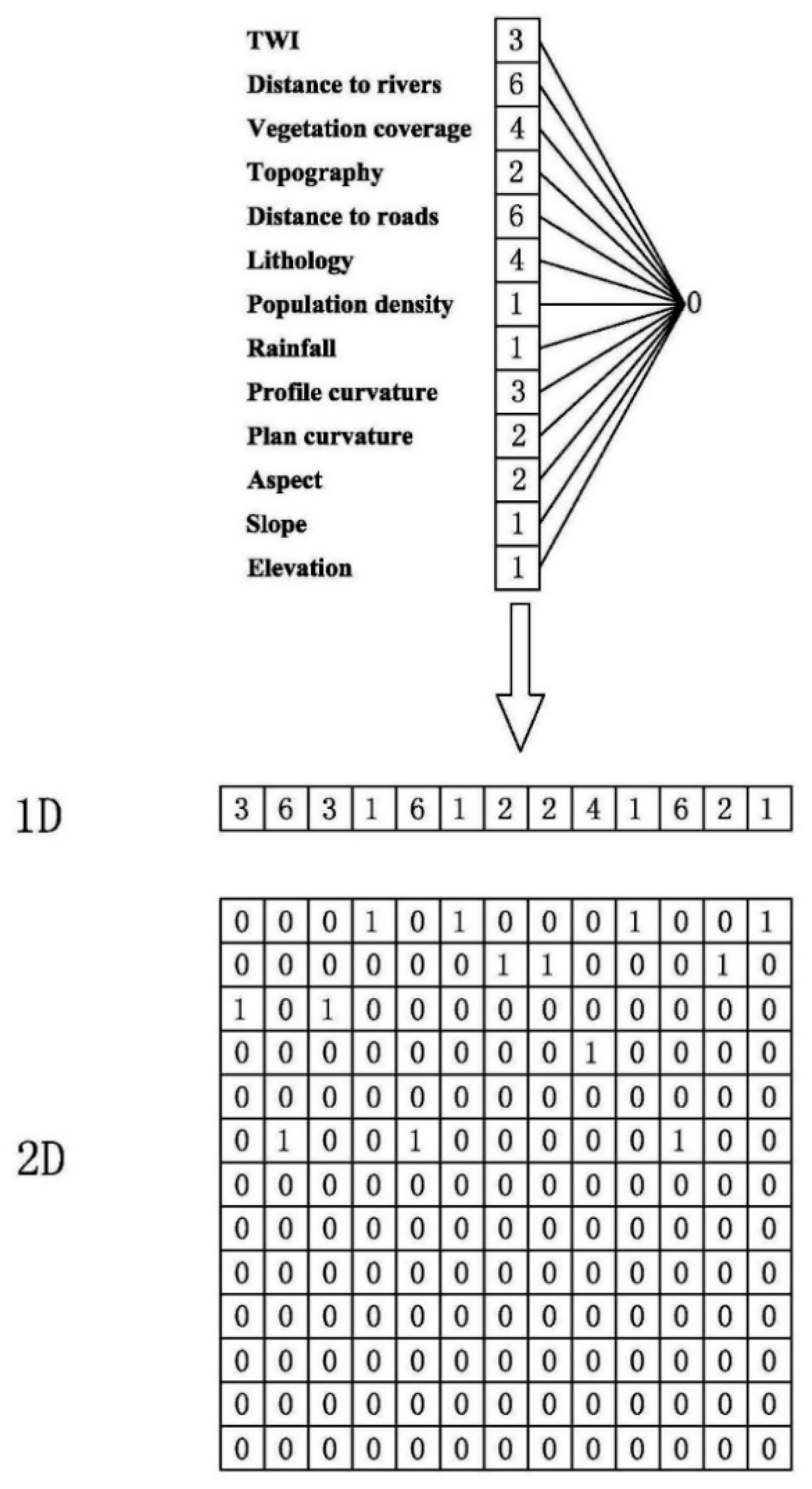
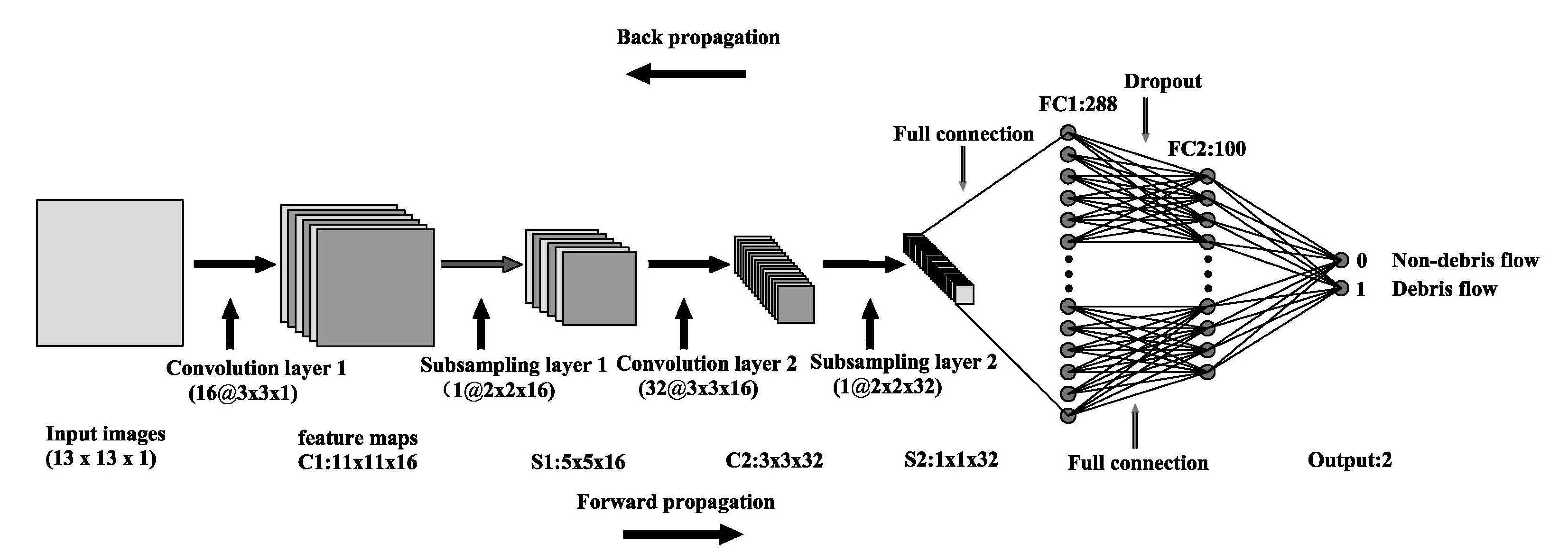
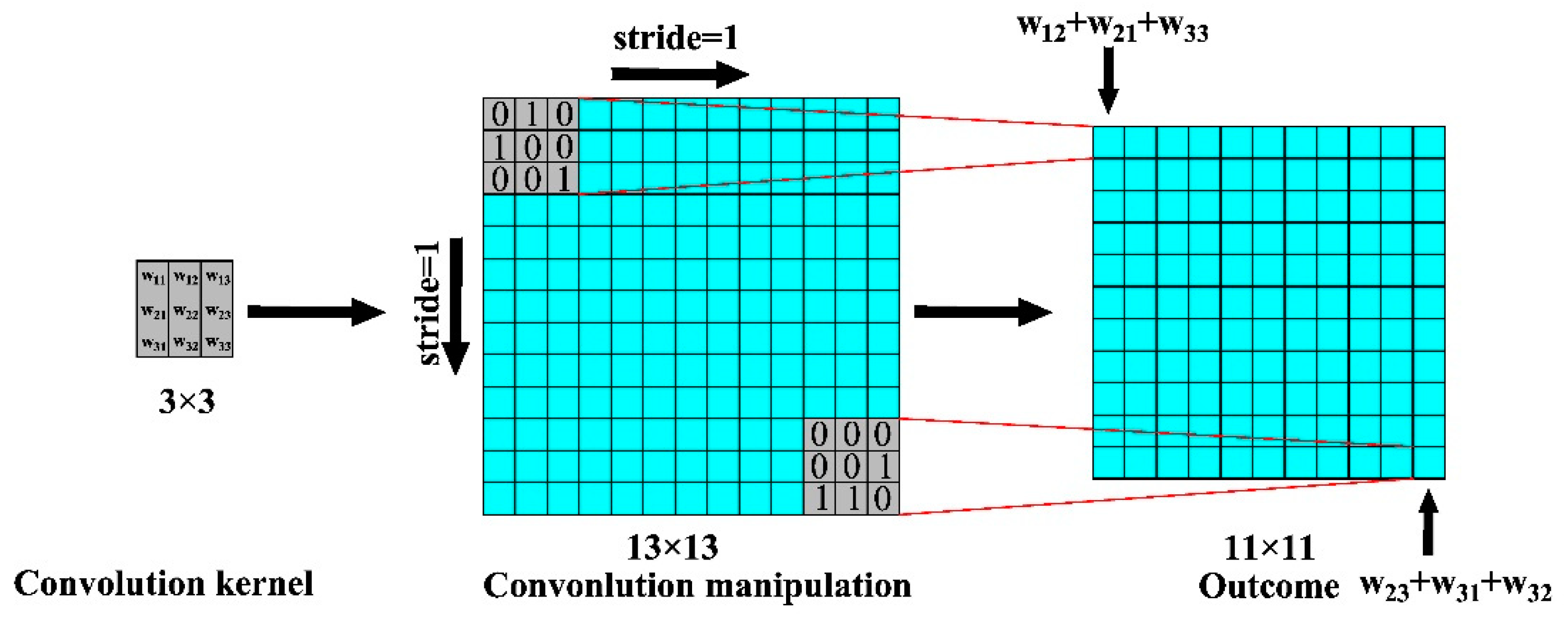
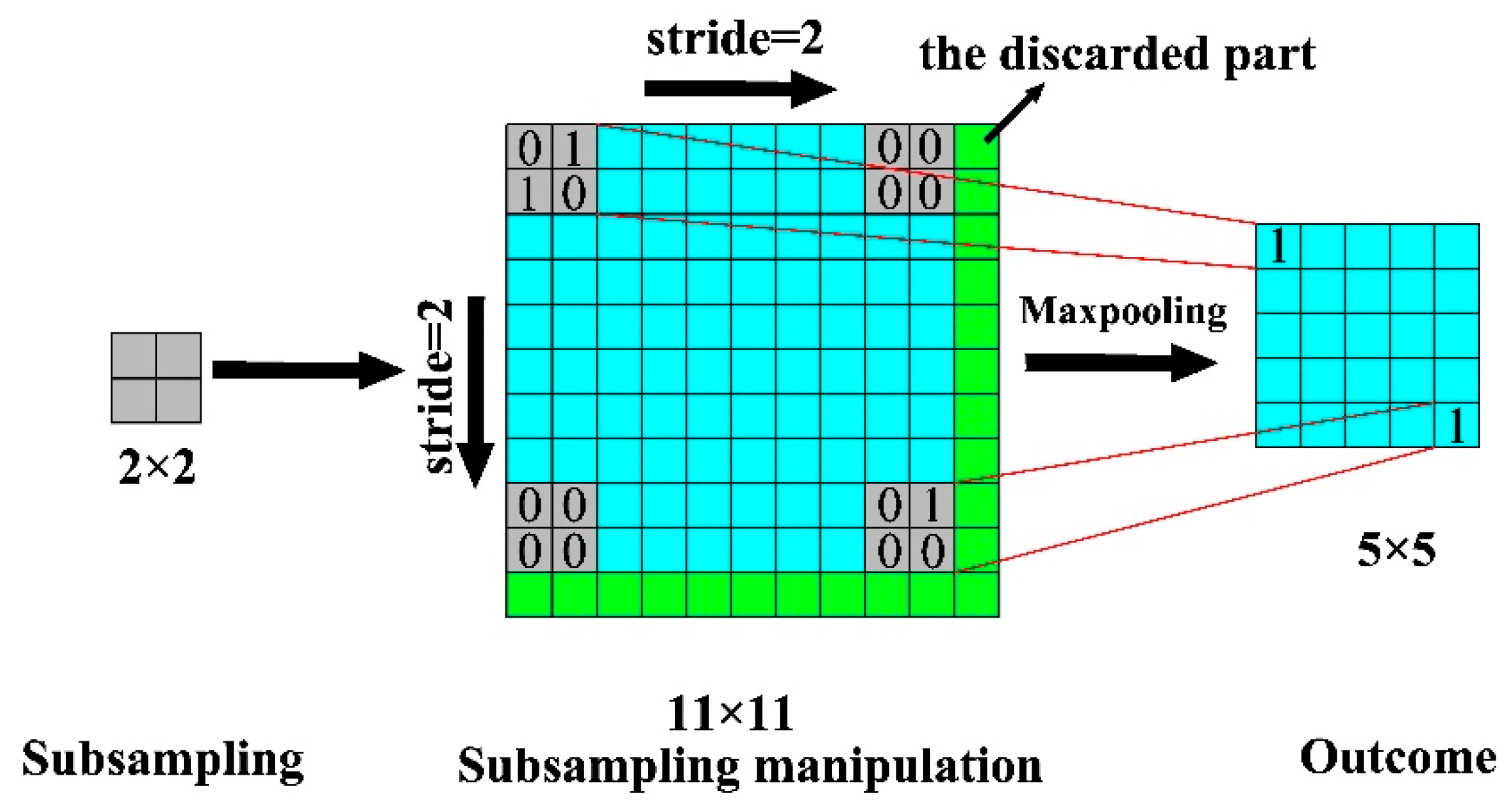
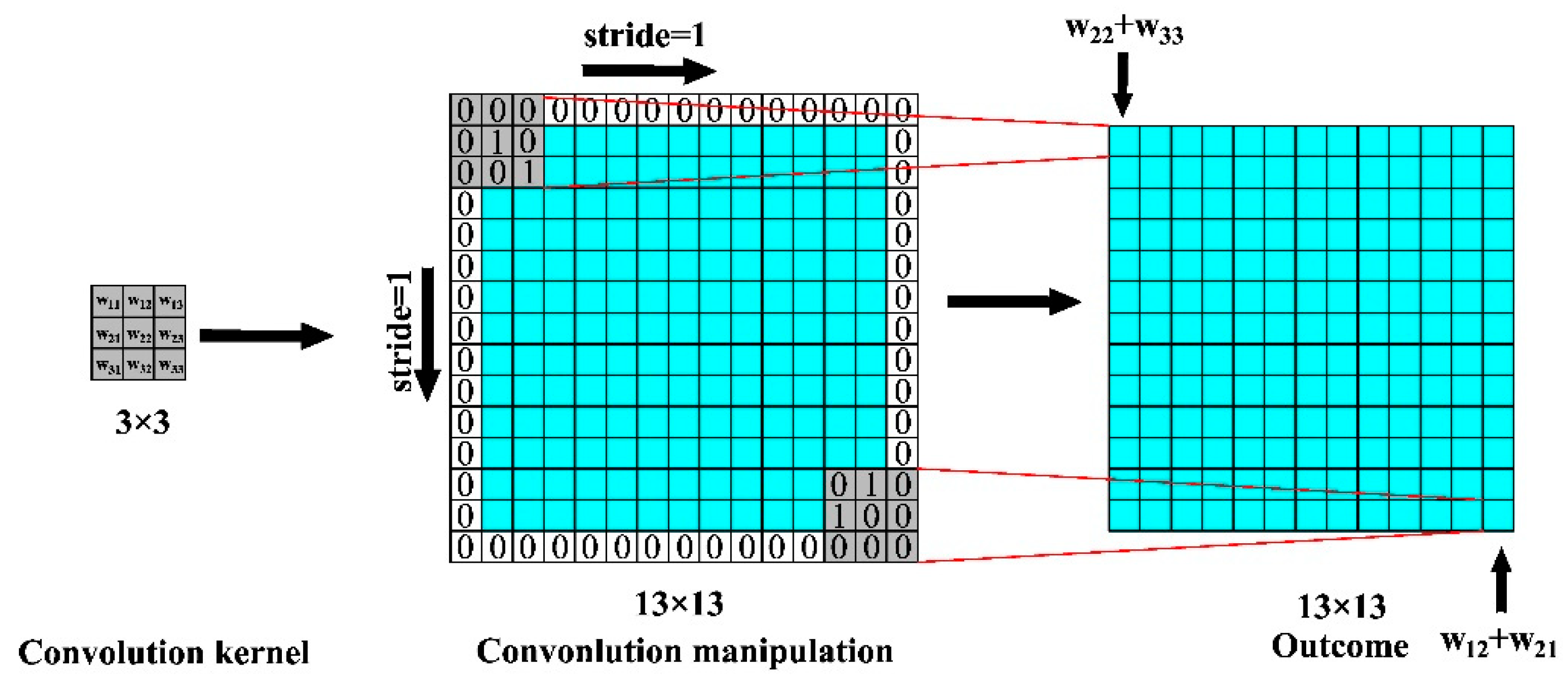
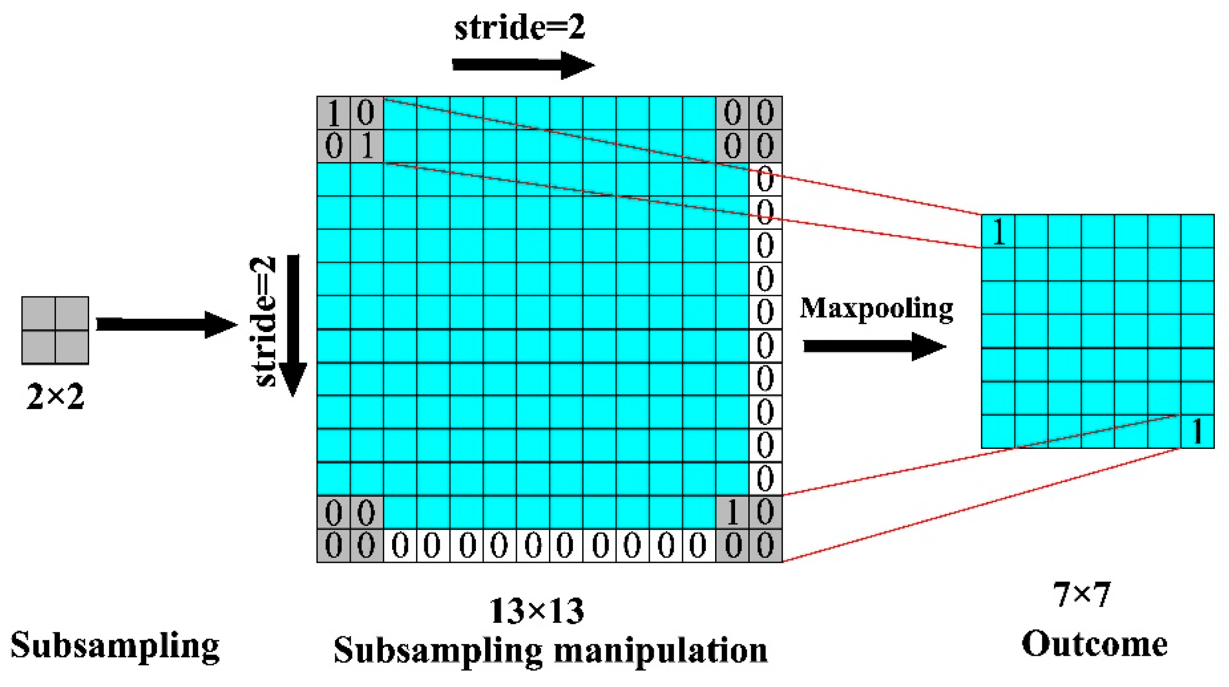
3.5. S–CNN
3.6. Model Evaluation
4. Results and Analysis
4.1. Multicollinearity Analysis Results
4.2. The Results of FR Method
4.3. The Results of GR Method
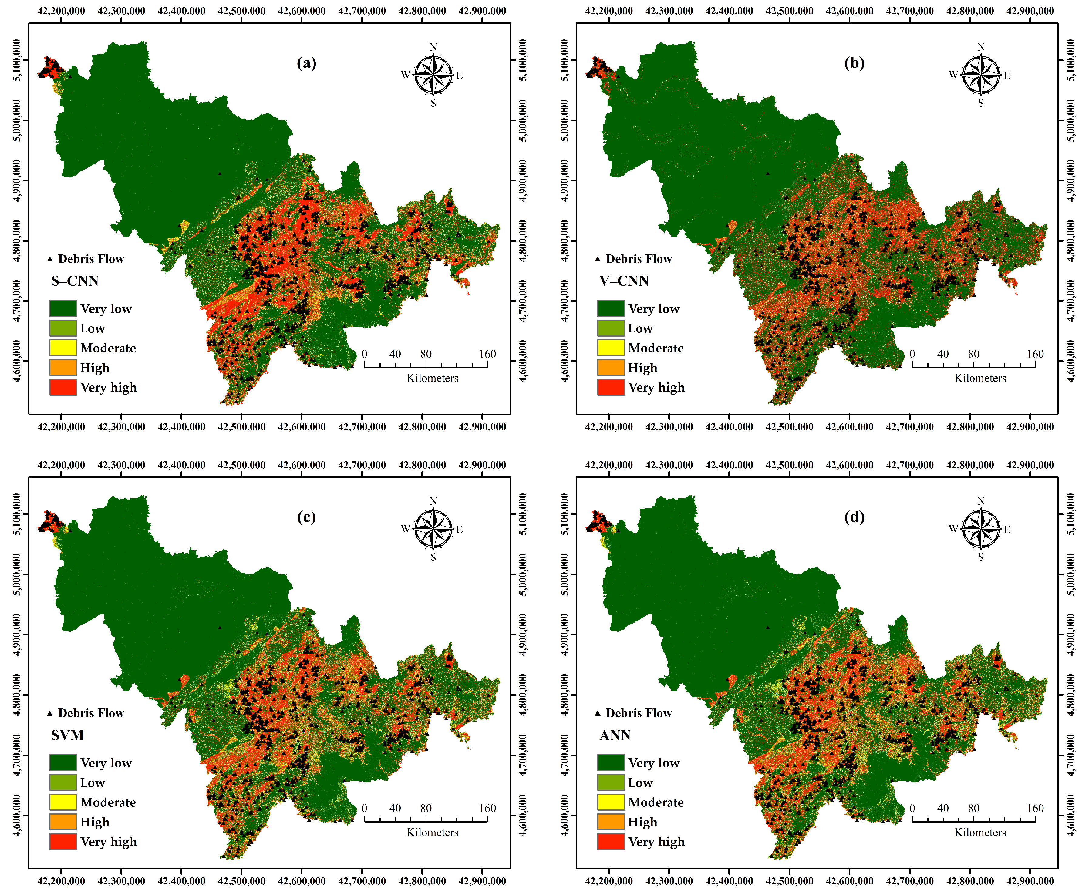
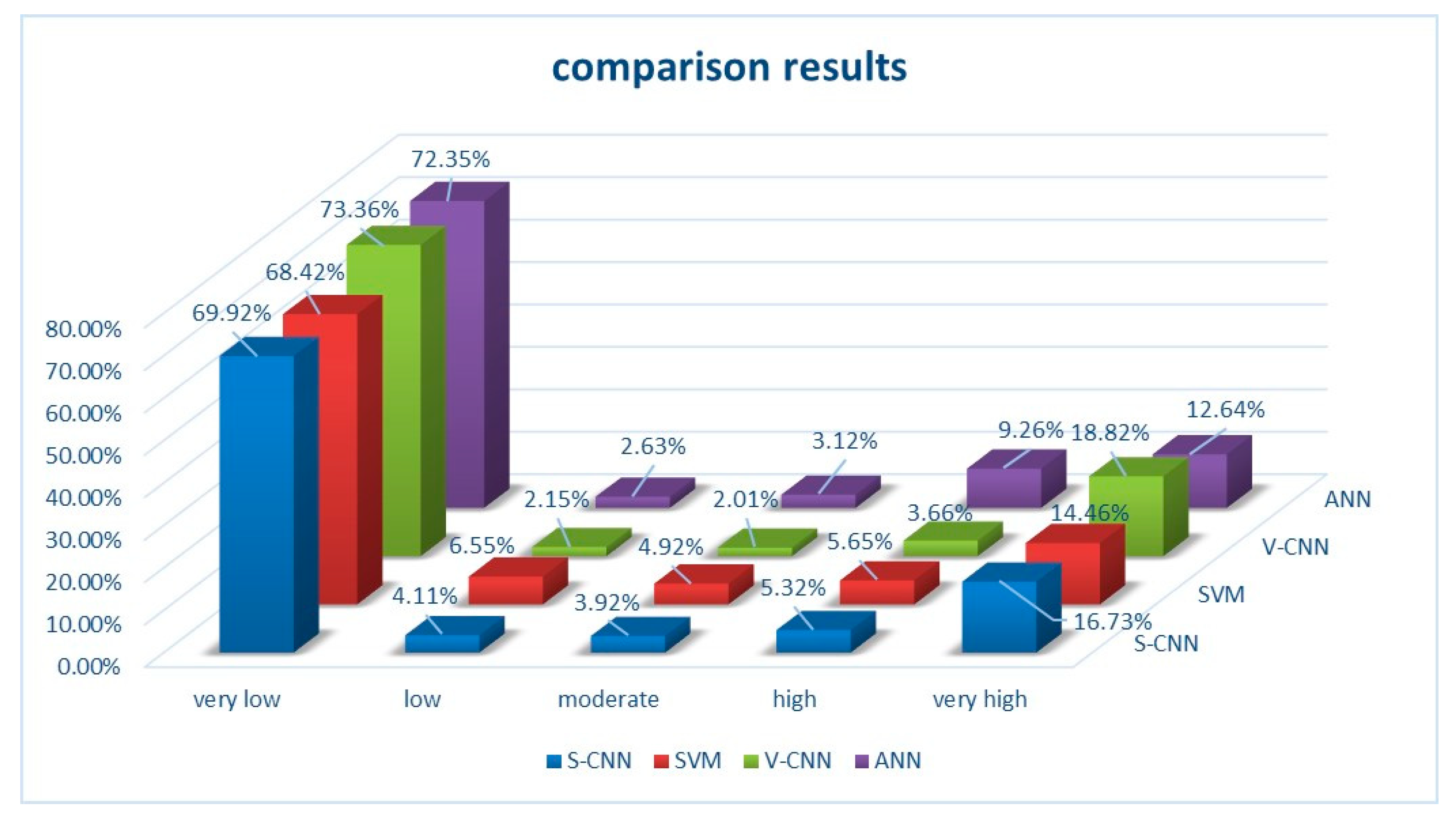
4.4. Production of the Debris Flow Susceptibility Maps
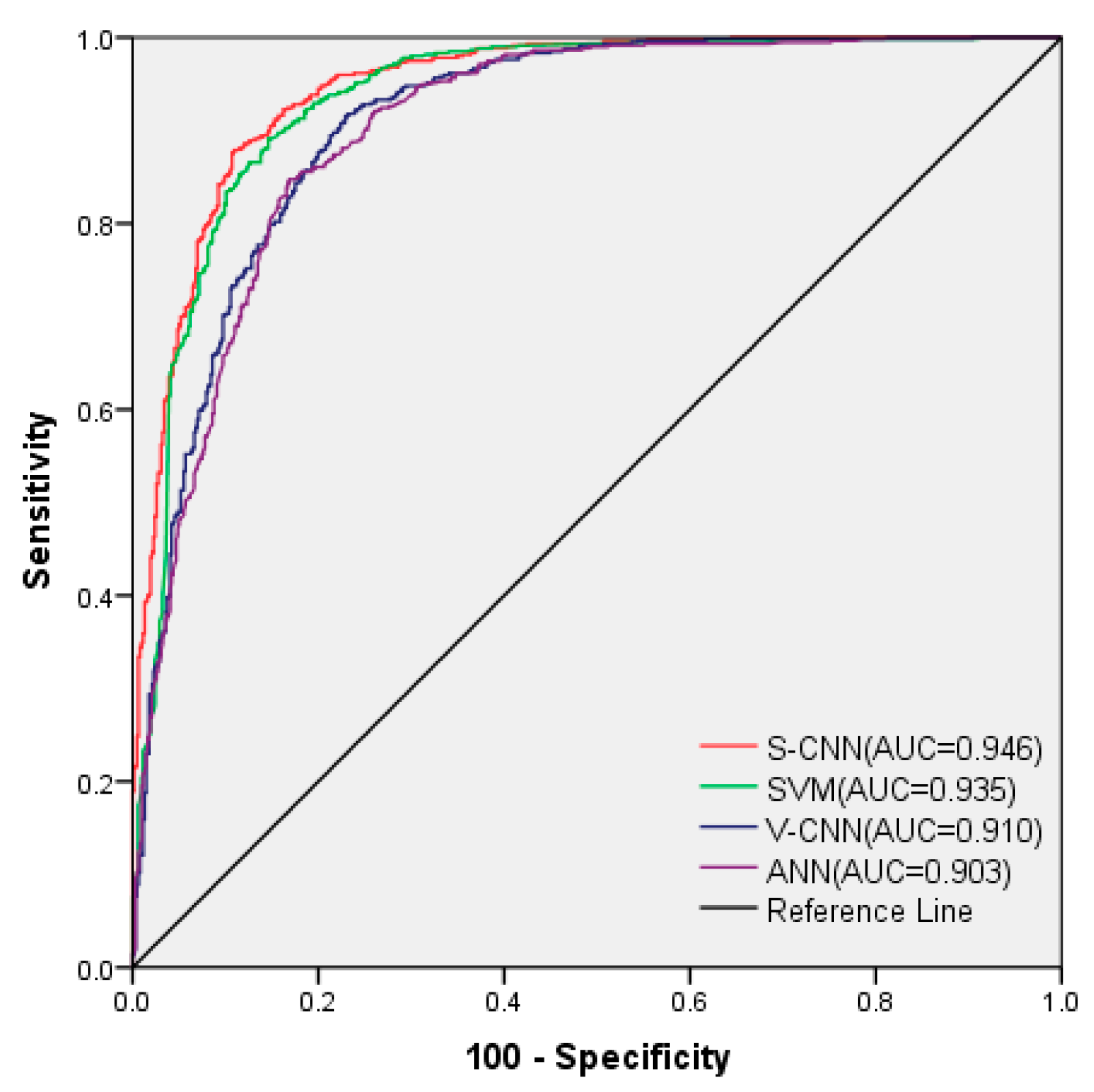
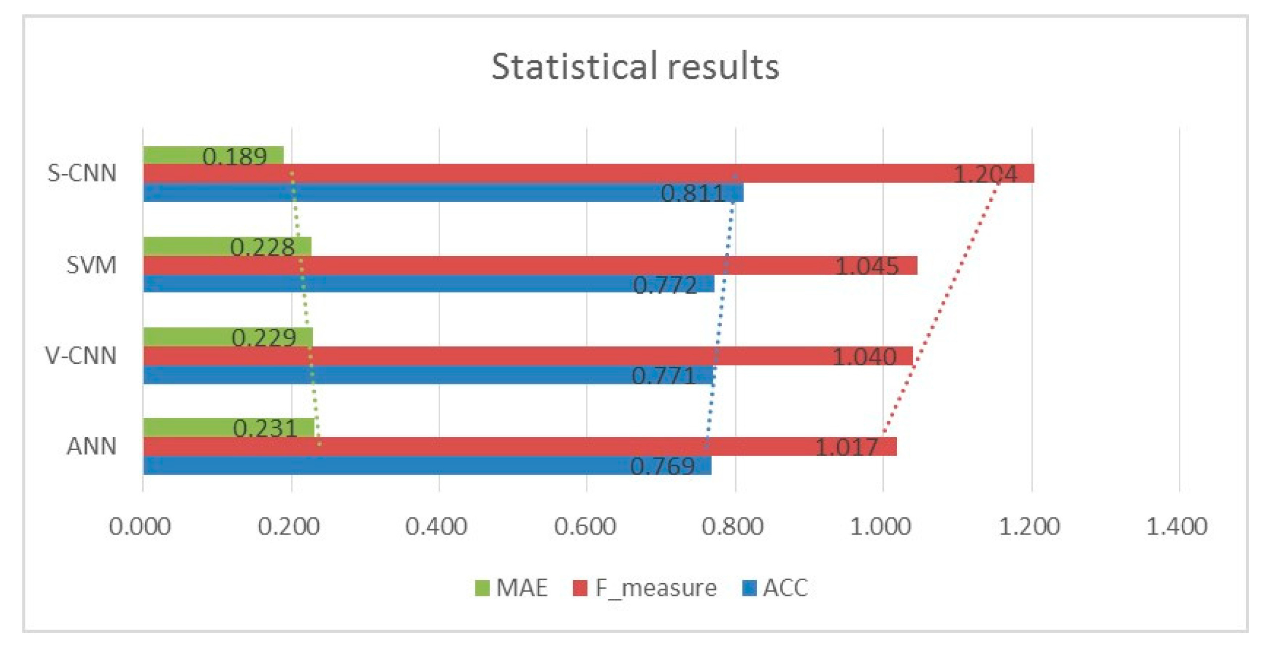
4.5. Model Validation
5. Discussion
6. Conclusions
- The AUC value of the V–CNN model (0.852) was higher than that of the ANN model (0.815). And three mathematical statistical methods also showed that the V–CNN model had smaller errors. The research indicated that the convolution layers and max pooling layers can extract more data patterns than pure full connection layers. Therefore, CNN models are more suitable for studying debris flow susceptibility than traditional ML methods such as ANN.
- The CNN models based on VALID padding still have some shortcomings. From the ROC caves and mathematical statistics, the accuracy of the V–CNN model was lower than that of the SVM model. This indicated that the method of VALID padding processing of the data was not the optimal choice. Therefore, SAME padding was selected to process debris flow data in this paper.
- SAME padding is more suitable for processing debris flow data compared with VALID padding. The S–CNN model obtained the highest AUC value and the minimum error. Obviously, the S–CNN model can make full use of the data and dig out more valuable information than the other three models.
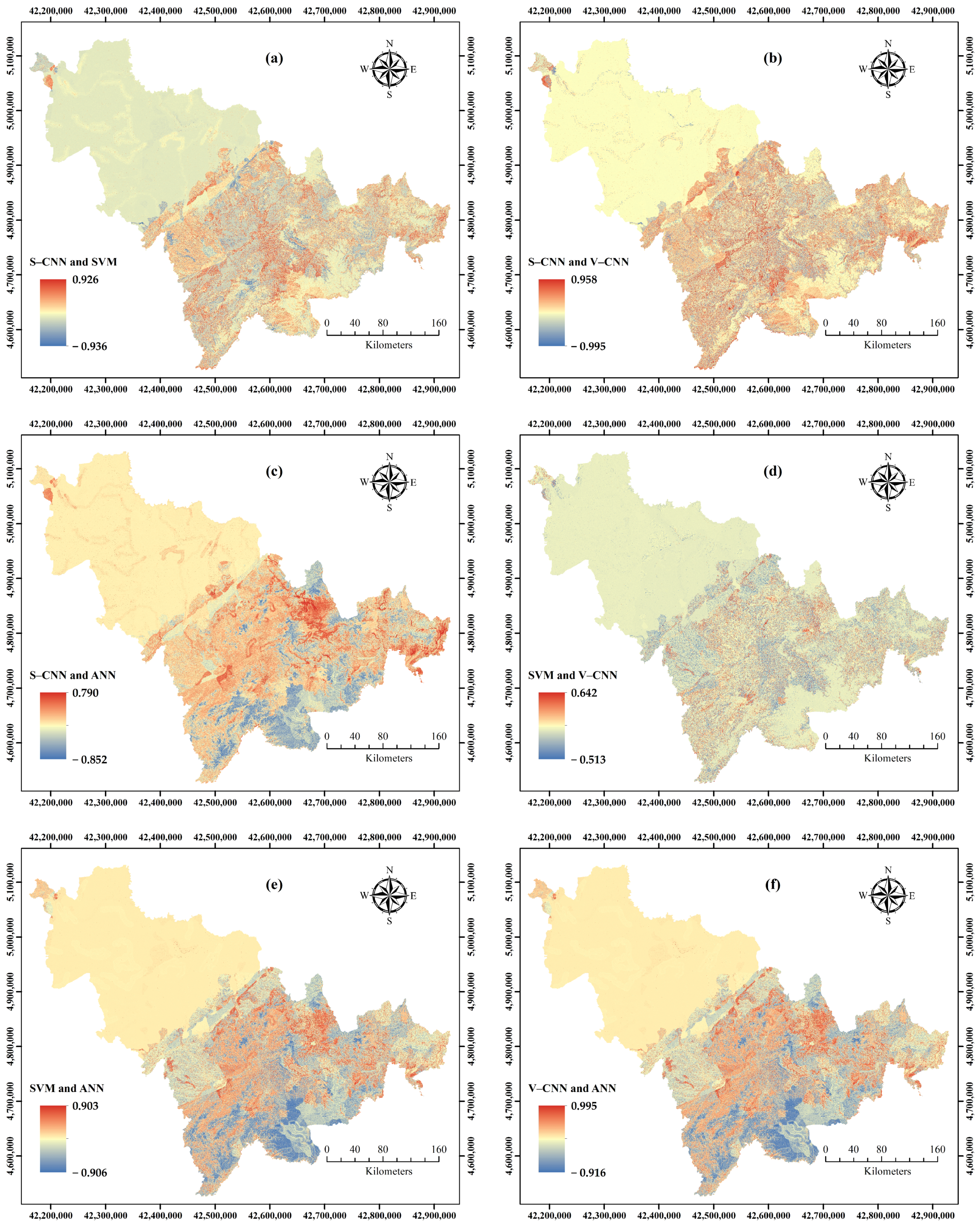
- We compare the susceptibility maps on a pixel–by–pixel basis and six comparison maps are produced. By observing the differences distribution of comparison maps, we draw a conclusion that the highest AUC map may not have the best predictive ability in some areas. This may be related to geotechnical and geomorphological reasons of differences and systematic errors.
Author Contributions
Funding
Conflicts of Interest
References
- Dowling, C.A.; Santi, P.M. Debris flows and their toll on human life: A global analysis of debris–flow fatalities from 1950 to 2011. Nat. Hazards 2014, 71, 203–227. [Google Scholar] [CrossRef]
- Xu, Q.; Zhang, S.; Li, W.L.; van Asch, T.W.J. The 13 August 2010 catastrophic debris flows after the 2008 Wenchuan earthquake, China. Nat. Hazards Earth Syst. Sci. 2012, 12, 201–216. [Google Scholar] [CrossRef]
- Iverson, R.M. Debris flows: Behavior and hazard assessment. Geol. Today 2014, 30, 15–20. [Google Scholar] [CrossRef]
- Zhou, G.G.D.; Cui, R.; Tang, J.B.; Chen, H.Y.; Zou, Q.; Sun, Q.C. Experimental study on the triggering mechanisms and kinematic properties of large debris flows in Wenjia Gully. Eng. Geol. 2015, 194, 52–61. [Google Scholar] [CrossRef]
- Westen, C.J.V.; Asch, T.W.J.V.; Soeters, R. Landslide hazard and risk zonation—why is it still so difficult? Bull. Eng. Geol. Environ. 2006, 65, 167–184. [Google Scholar] [CrossRef]
- Brabb, E.E. Innovative approaches to landslide hazard mapping. In Proceedings of the Fourth International Symposium on Landslides, Canadian Geotechnical Society, Toronto, SD, Canada, 16–21 September 1984; pp. 307–324. [Google Scholar]
- Reichenbach, P.; Rossi, M.; Malamud, B.D.; Mihir, M.; Guzzetti, F. A review of statistically–based landslide susceptibility models. Earth-Sci. Rev. 2018, 180, 60–91. [Google Scholar] [CrossRef]
- Pourghasemi, H.R.; Yansari, Z.T.; Panagos, P.; Pradhan, B. Analysis and evaluation of landslide susceptibility: A review on articles published during 2005–2016 (periods of 2005–2012 and 2013–2016). Arab. J. Geosci. 2018, 11, 193. [Google Scholar] [CrossRef]
- Wu, Y.; Li, W.; Liu, P.; Bai, H.; Wang, Q.; He, J.; Liu, Y.; Sun, S. Application of analytic hierarchy process model for landslide susceptibility mapping in the Gangu County, Gansu Province, China. Environ. Earth Sci. 2016, 75, 422. [Google Scholar] [CrossRef]
- Quan, H.; Lee, B. GIS–based landslide susceptibility mapping using analytic hierarchy process and artificial neural network in Jeju (Korea). KSCE J. Civ. Eng. 2012, 16, 1258–1266. [Google Scholar] [CrossRef]
- Quan, H.; Moon, H.D.; Jin, G. Landslide Susceptibility Analysis in Baekdu Mountain Area Using ANN and AHP Method. J. Korean Geoenviron. Soc. 2014, 15, 79–85. [Google Scholar] [CrossRef] [Green Version]
- Dhianaufal, D.; Kristyanto, T.H.W.; Indra, T.L.; Syahputra, R. Fuzzy Logic Method for Landslide Susceptibility Mapping in Volcanic Sediment Area in Western Bogor. AIP Conf. Proc. 2018, 2023, 020190. [Google Scholar] [CrossRef]
- Basofi, A.; Fariza, A.; Dzulkarnain, M.R. Landslides Susceptibility Mapping Using Fuzzy Logic: A Case Study in Ponorogo. In Proceedings of the 2016 International Conference on Data and Software Engineering (ICoDSE), East Java, Indonesia, 26–27 October 2016. [Google Scholar]
- Pradhan, B. Use of GIS–based fuzzy logic relations and its cross application to produce landslide susceptibility maps in three test areas in Malaysia. Environ. Earth Sci. 2011, 63, 329–349. [Google Scholar] [CrossRef]
- Hong, H.; Ilia, I.; Tsangaratos, P.; Chen, W.; Xu, C. A hybrid fuzzy weight of evidence method in landslide susceptibility analysis on the Wuyuan area, China. Geomorphology 2017, 290, 1–16. [Google Scholar] [CrossRef]
- Regmi, A.D.; Yoshida, K.; Pourghasemi, H.R.; Dhital, M.R.; Pradhan, B. Landslide susceptibility mapping along Bhalubang—Shiwapur area of mid–Western Nepal using frequency ratio and conditional probability models. J. Mt. Sci. 2014, 11, 1266–1285. [Google Scholar] [CrossRef]
- Razavizadeh, S.; Solaimani, K.; Massironi, M.; Kavian, A. Mapping landslide susceptibility with frequency ratio, statistical index, and weights of evidence models: A case study in northern Iran. Environ. Earth Sci. 2017, 76, 499. [Google Scholar] [CrossRef]
- Huang, F.; Cao, Z.; Guo, J.; Jiang, S.; Li, S.; Guo, Z. Comparisons of heuristic, general statistical and machine learning models for landslide susceptibility prediction and mapping. Catena 2020, 191, 104580. [Google Scholar] [CrossRef]
- Aditian, A.; Kubota, T.; Shinohara, Y. Comparison of GIS–based landslide susceptibility models using frequency ratio, logistic regression, and artificial neural network in a tertiary region of Ambon, Indonesia. Geomorphology 2018, 318, 101–111. [Google Scholar] [CrossRef]
- Kavzoglu, T.; Sahin, E.K.; Colkesen, I. Landslide susceptibility mapping using GIS–based multi–criteria decision analysis, support vector machines, and logistic regression. Landslides 2014, 11, 425–439. [Google Scholar] [CrossRef]
- Kumar, D.; Thakur, M.; Dubey, C.S.; Shukla, D.P. Landslide susceptibility mapping & prediction using Support Vector Machine for Mandakini River Basin, Garhwal Himalaya, India. Geomorphology 2017, 295, 115–125. [Google Scholar]
- Kalantar, B.; Pradhan, B.; Naghibi, S.A.; Motevalli, A.; Mansor, S. Assessment of the effects of training data selection on the landslide susceptibility mapping: A comparison between support vector machine (SVM), logistic regression (LR) and artificial neural networks (ANN). Geomat. Nat. Hazards Risk 2018, 9, 49–69. [Google Scholar] [CrossRef]
- Tsangaratos, P.; Ilia, I. Comparison of a logistic regression and Naive Bayes classifier in landslide susceptibility assessments: The influence of models complexity and training dataset size. Catena 2016, 145, 164–179. [Google Scholar] [CrossRef]
- Gelisli, K.; Kaya, T.; Babacan, A.E. Assessing the factor of safety using an artificial neural network: Case studies on landslides in Giresun, Turkey. Environ. Earth Sci. 2015, 73, 8639–8646. [Google Scholar] [CrossRef]
- Dieu, T.B.; Tran, A.T.; Klempe, H.; Pradhan, B.; Revhaug, I. Spatial prediction models for shallow landslide hazards: A comparative assessment of the efficacy of support vector machines, artificial neural networks, kernel logistic regression, and logistic model tree. Landslides 2016, 13, 361–378. [Google Scholar]
- Pourghasemi, H.R.; Kerle, N. Random forests and evidential belief function–based landslide susceptibility assessment in Western Mazandaran Province, Iran. Environ. Earth Sci. 2016, 75. [Google Scholar] [CrossRef]
- Kim, J.; Lee, S.; Jung, H.; Lee, S. Landslide susceptibility mapping using random forest and boosted tree models in Pyeong–Chang, Korea. Geocarto Int. 2018, 33, 1000–1015. [Google Scholar] [CrossRef]
- Xiong, K.; Adhikari, B.R.; Stamatopoulos, C.A.; Zhan, Y.; Wu, S.; Dong, Z.; Di, B. Comparison of Different Machine Learning Methods for Debris Flow Susceptibility Mapping: A Case Study in the Sichuan Province, China. Remote Sens. 2020, 12, 295. [Google Scholar] [CrossRef] [Green Version]
- Esper Angillieri, M.Y. Debris flow susceptibility mapping in a portion of the Andes and Preandes of San Juan, Argentina using frequency ratio and logistic regression models. Earth Sci. Res. J. 2013, 17, 159–167. [Google Scholar]
- Wang, Y.; Fang, Z.C.; Hong, H.Y. Comparison of convolutional neural networks for landslide susceptibility mapping in Yanshan County, China. Sci. Total Environ. 2019, 666, 975–993. [Google Scholar] [CrossRef]
- Ma, Z.; Qin, S.; Cao, C.; Lv, J.; Li, G.; Qiao, S.; Hu, X. The Influence of Different Knowledge–Driven Methods on Landslide Susceptibility Mapping: A Case Study in the Changbai Mountain Area, Northeast China. Entropy 2019, 21, 372. [Google Scholar] [CrossRef] [Green Version]
- Qiao, S.; Qin, S.; Chen, J.; Hu, X.; Ma, Z. The Application of a Three-Dimensional Deterministic Model in the Study of Debris Flow Prediction Based on the Rainfall–Unstable Soil Coupling Mechanism. Processes 2019, 7, 99. [Google Scholar] [CrossRef] [Green Version]
- Ghorbanzadeh, O.; Blaschke, T.; Gholamnia, K.; Meena, S.R.; Tiede, D.; Aryal, J. Evaluation of Different Machine Learning Methods and Deep–Learning Convolutional Neural Networks for Landslide Detection. Remote Sens. 2019, 11, 196. [Google Scholar] [CrossRef] [Green Version]
- Vu, D.P.; Quoc–Huy, N.; Huu–Duy, N.; Van–Manh, P.; Van Manh, V.; Quang–Thanh, B. Convolutional Neural Network & x2014; Optimized Moth Flame Algorithm for Shallow Landslide Susceptible Analysis. IEEE Access 2020, 8, 32727–32736. [Google Scholar]
- Ullo, S.L.; Langenkamp, M.S.; Oikarinen, T.P.; Del Rosso, M.P.; Sebastianelli, A.; Piccirillo, F.; Sica, S. Landslide Geohazard Assessment With Convolutional Neural Networks Using Sentinel–2 Imagery Data. In Proceedings of the IEEE International Symposium on Geoscience and Remote Sensing IGARSS, Yokohama, Japan, 28 July–2 August 2019. [Google Scholar] [CrossRef] [Green Version]
- Cheng, G.; Ma, C.; Zhou, P.; Yao, X.; Han, J. Scene classification of high resolution remote sensing images using convolutional neural networks. In Proceedings of the 2016 IEEE International Geoscience and Remote Sensing Symposium (IGARSS), Beijing, China, 10–15 July 2016. [Google Scholar]
- Krizhevsky, A.; Sutskever, I.; Hinton, G. ImageNet Classification with Deep Convolutional Neural Networks. Adv. Neural Inf. Process. Syst. 2012, 25, 6. [Google Scholar] [CrossRef]
- Galli, M.; Ardizzone, F.; Cardinali, M.; Guzzetti, F.; Reichenbach, P. Comparing landslide inventory maps. Geomorphology 2008, 94, 268–289. [Google Scholar] [CrossRef]
- Guzzetti, F.; Mondini, A.C.; Cardinali, M.; Fiorucci, F.; Santangelo, M.; Chang, K. Landslide inventory maps: New tools for an old problem. Earth-Sci. Rev. 2012, 112, 42–66. [Google Scholar] [CrossRef] [Green Version]
- Dou, Q.; Qin, S.W.; Zhang, Y.C.; MA, Z.J.; Chen, J.; Qiao, S.; Hu, X.; Liu, F. A Method for Improving Controlling Factors Based on Information Fusion for Debris Flow Susceptibility Mapping: A Case Study in Jilin Province, China. Entropy 2019, 21, 695. [Google Scholar] [CrossRef] [Green Version]
- Conforti, M.; Pascale, S.; Robustelli, G.; Sdao, F. Evaluation of prediction capability of the artificial neural networks for mapping landslide susceptibility in the Turbolo River catchment (northern Calabria, Italy). Catena 2014, 113, 236–250. [Google Scholar] [CrossRef]
- Pant, A.K.P.A. Landslide hazard mapping based on geological attributes. Eng. Geol. 1992, 32, 81–100. [Google Scholar]
- Süzen, M.L.; Doyuran, V. Data driven bivariate landslide susceptibility assessment using geographical information systems: A method and application to Asarsuyu catchment, Turkey. Eng. Geol. 2004, 71, 303–321. [Google Scholar] [CrossRef]
- Lee, S.; Min, K. Statistical analysis of landslide susceptibility at Yongin, Korea. Environ. Geol. 2001, 40, 1095–1113. [Google Scholar] [CrossRef]
- De Vita, P.; Napolitano, E.; Godt, J.W.; Baum, R.L. Deterministic estimation of hydrological thresholds for shallow landslide initiation and slope stability models: Case study from the Somma–Vesuvius area of southern Italy. Landslides 2013, 10, 713–728. [Google Scholar] [CrossRef]
- Aksoy, B.; Ercanoglu, M. Landslide identification and classification by object–based image analysis and fuzzy logic: An example from the Azdavay region (Kastamonu, Turkey). Comput. Geosci. 2012, 38, 87–98. [Google Scholar] [CrossRef]
- Cevik, E.; Topal, T. GIS–based landslide susceptibility mapping for a problematic segment of the natural gas pipeline, Hendek (Turkey). Environ. Geol. 2003, 44, 949–962. [Google Scholar] [CrossRef]
- Dou, J.; Yunus, A.P.; Dieu, T.B.; Sahana, M.; Chen, C.; Zhu, Z.; Wang, W.; Binh, T.P. Evaluating GIS–Based Multiple Statistical Models and Data Mining for Earthquake and Rainfall–Induced Landslide Susceptibility Using the LiDAR DEM. Remote Sens. 2019, 11, 638. [Google Scholar] [CrossRef] [Green Version]
- Fernandes, N.F.; Guimares, R.F.; Gomes, R.A.T.; Vieira, B.C.; Greenberg, H. Topographic controls of landslides in Rio de Janeiro: Field evidence and modeling. Catena 2004, 55, 163–181. [Google Scholar] [CrossRef]
- Nefeslioglu, H.A.; Duman, T.Y.; Durmaz, S. Landslide susceptibility mapping for a part of tectonic Kelkit Valley (Eastern Black Sea region of Turkey). Geomorphology 2008, 94, 401–418. [Google Scholar] [CrossRef]
- He, Q.; Shahabi, H.; Shirzadi, A.; Li, S.; Chen, W.; Wang, N.; Chai, H.; Bian, H.; Ma, J.; Chen, Y.; et al. Landslide spatial modelling using novel bivariate statistical based Naive Bayes, RBF Classifier, and RBF Network machine learning algorithms. Sci. Total Environ. 2019, 663, 1–15. [Google Scholar] [CrossRef]
- Dai, F.C.; Lee, C.F.; Li, J.; Xu, Z.W. Assessment of landslide susceptibility on the natural terrain of Lantau Island, Hong Kong. Environ. Geol. 2001, 40, 381–391. [Google Scholar]
- Segoni, S.; Pappafico, G.; Luti, T.; Catani, F. Landslide susceptibility assessment in complex geological settings: Sensitivity to geological information and insights on its parameterization. Landslides 2020. [Google Scholar] [CrossRef] [Green Version]
- Pachauri, A.K.; Gupta, P.V.; Chander, R. Landslide zoning in a part of the Garhwal Himalayas. Environ. Geol. 1998, 36, 325–334. [Google Scholar] [CrossRef]
- Song, Y.; Gong, J.; Sheng, G.; Wang, D.; Cui, T.; Yi, L.; Wei, B. Susceptibility assessment of earthquake–induced landslides using Bayesian network: A case study in Beichuan, China. Comput. Geosci. 2012, 42, 189–199. [Google Scholar] [CrossRef]
- Gan, B.; Liu, X.; Yang, X.; Wang, X.; Zhou, J. The impact of human activities on the occurrence of mountain flood hazards: Lessons from the 17 August 2015 flash flood/debris flow event in Xuyong County, south–western China. Geomat. Nat. Hazards Risk 2018, 9, 816–840. [Google Scholar] [CrossRef] [Green Version]
- Nguyen, T.L.; De Smedt, F. Analysis and Mapping of Rainfall–Induced Landslide Susceptibility in A Luoi District, Thua Thien Hue Province, Vietnam. Water 2019, 11, 51. [Google Scholar]
- Yu, B.; Wang, T.; Zhu, Y.; Zhu, Y. Topographical and rainfall factors determining the formation of gully–type debris flows caused by shallow landslides in the Dayi area, Guizhou Province, China. Environ. Earth Sci. 2016, 75, 551. [Google Scholar] [CrossRef]
- Chen, W.; Yan, X.; Zhao, Z.; Hong, H.; Bui, D.T.; Pradhan, B. Spatial prediction of landslide susceptibility using data mining–based kernel logistic regression, naive Bayes and RBFNetwork models for the Long County area (China). Bull. Eng. Geol. Environ. 2019, 78, 247–266. [Google Scholar] [CrossRef]
- Dou, J.; Yunus, A.P.; Dieu, T.B.; Merghadi, A.; Sahana, M.; Zhu, Z.; Chen, C.; Khosravi, K.; Yang, Y.; Binh, T.P. Assessment of advanced random forest and decision tree algorithms for modeling rainfall–induced landslide susceptibility in the Izu–Oshima Volcanic Island, Japan. Sci. Total Environ. 2019, 662, 332–346. [Google Scholar] [CrossRef]
- O’Brien, R.M. A caution regarding rules of thumb for variance inflation factors. Qual. Quant. 2007, 41, 673–690. [Google Scholar] [CrossRef]
- Al-Juaidi, A.E.M.; Nassar, A.M.; Al-Juaidi, O.E.M. Evaluation of flood susceptibility mapping using logistic regression and GIS conditioning factors. Arab. J. Geosci. 2018, 11, 1–10. [Google Scholar] [CrossRef]
- Kumar, A.; Sharma, R.K.; Bansal, V.K. GIS–based comparative study of information value and frequency ratio method for landslide hazard zonation in a part of mid–Himalaya in Himachal Pradesh. Innov. Infrastruct. Solut. 2019, 4, 28. [Google Scholar] [CrossRef]
- Quinlan, J.R. Programs for Machine Learning; Morgan Kaufmann Publishers Inc.: Burlington, MA, USA, 1992. [Google Scholar]
- Lecun, Y.; Bottou, L.; Bengio, Y.; Haffner, P. Gradient–based learning applied to document recognition. Proc. IEEE 1998, 86, 2278–2324. [Google Scholar] [CrossRef] [Green Version]
- Chung, C.; Fabbri, A.G. Validation of spatial prediction models for landslide hazard mapping. Nat. Hazards 2003, 30, 451–472. [Google Scholar] [CrossRef]
- Cantarino, I.; Angel Carrion, M.; Goerlich, F.; Martinez Ibanez, V. A ROC analysis–based classification method for landslide susceptibility maps. Landslides 2019, 16, 265–282. [Google Scholar] [CrossRef]
- Chen, W.; Zhang, S.; Li, R.; Shahabi, H. Performance evaluation of the GIS–based data mining techniques of best–first decision tree, random forest, and naive Bayes tree for landslide susceptibility modeling. Sci. Total Environ. 2018, 644, 1006–1018. [Google Scholar] [CrossRef] [PubMed]
- Oh, H.; Pradhan, B. Application of a neuro–fuzzy model to landslide–susceptibility mapping for shallow landslides in a tropical hilly area. Comput. Geosci. 2011, 37, 1264–1276. [Google Scholar] [CrossRef]
- Albatayneh, O.; Forslof, L.; Ksaibati, K. Image Retraining Using TensorFlow Implementation of the Pretrained Inception–v3 Model for Evaluating Gravel Road Dust. J. Infrastruct. Syst. 2020, 26, 2. [Google Scholar] [CrossRef]
- Khan, M.N.; Ahmed, M.M. Trajectory–level fog detection based on in–vehicle video camera with TensorFlow deep learning utilizing SHRP2 naturalistic driving data. Accid. Anal. Prev. 2020, 142, 105521. [Google Scholar] [CrossRef]
- Lin, G.; Chang, M.; Huang, Y.; Ho, J. Assessment of susceptibility to rainfall–induced landslides using improved self–organizing linear output map, support vector machine, and logistic regression. Eng. Geol. 2017, 224, 62–74. [Google Scholar] [CrossRef]
- Chen, W.; Chai, H.; Zhao, Z.; Wang, Q.; Hong, H. Landslide susceptibility mapping based on GIS and support vector machine models for the Qianyang County, China. Environ. Earth Sci. 2016, 75, 6. [Google Scholar] [CrossRef]
- Huang, Y.; Zhao, L. Review on landslide susceptibility mapping using support vector machines. Catena 2018, 165, 520–529. [Google Scholar] [CrossRef]
- Can, A.; Dagdelenler, G.; Ercanoglu, M.; Sonmez, H. Landslide susceptibility mapping at Ovack–Karabuk (Turkey) using different artificial neural network models: Comparison of training algorithms. Bull. Eng. Geol. Environ. 2019, 78, 89–102. [Google Scholar] [CrossRef]
- Chauhan, S.; Sharma, M.; Arora, M.K.; Gupta, N.K. Landslide Susceptibility Zonation through ratings derived from Artificial Neural Network. Int. J. Appl. Earth Obs. Geoinf. 2010, 12, 340–350. [Google Scholar] [CrossRef]
- Tian, Y.; Xu, C.; Hong, H.; Zhou, Q.; Wang, D. Mapping earthquake–triggered landslide susceptibility by use of artificial neural network (ANN) models: An example of the 2013 Minxian (China) Mw 5.9 event. Geomat. Nat. Hazards Risk 2019, 10, 1–25. [Google Scholar] [CrossRef] [Green Version]
- Xiao, T.; Segoni, S.; Chen, L.; Yin, K.; Casagli, N. A step beyond landslide susceptibility maps: A simple method to investigate and explain the different outcomes obtained by different approaches. Landslides 2020, 17, 627–640. [Google Scholar] [CrossRef] [Green Version]


| System | Stratum Code | Group | Main Lithology |
|---|---|---|---|
| Archean eon | Ar1 | Yangjiadian | Dark black, columnar structure, including plagioclase, hornblende, pyroxene |
| Ar2 | Laoniugou | Pyroxene granulite, hornblende metagranite, pyroxene magnetite rock | |
| Proterozoic eon | Pt1 | Linjiang | The phyllite, sericite phyllite and diorite schist |
| Cambrian Period | Є1 | Changping | Gray medium–thin limestone, asphaltene limestone, dolomite limestone |
| Є2 | Zhangxia | Blue–grey bioclastic limestone, gray thin layered limestone | |
| Є3 | Gushan | Purple siltstone, shale with thin limestone | |
| Ordovician period | O1 | Majiagou | Light gray dolomite limestone, flint nodular limestone |
| Silurian Period | S1 | Taoshan | Gray, dark gray fine sandstone, siltstone, silty slate with mud limestone. |
| Devonian Period | D2 | Wangjiajie | Gray medium–thick layer limestone, bioclastic limestone |
| Carboniferous Period | C2 | Shanxi | Dark coarse sandstone, siltstone, shale, and coal, with a thin layer of limestone |
| Permian period | P2 | Sunjiagou | Red mudstone, silty mudstone, and feldspar sandstone |
| Triassic Period | T3 | Daxinggou | Volcanic rocks with sedimentary clastic rocks and thin coal seams |
| Jurassic Period | J1 | Hongqi | Sandstone, siltstone, mudstone |
| J2 | Wanbao | Sandstone, siltstone, carbonaceous mudstone | |
| J3 | Shahezi | Gray sandstone, siltstone with five layers of coal | |
| Cretaceous period | K1 | Yaojia | Interlayer of brown–red mudstone and gray–green mudstone, siltstone |
| K2 | Nenjiang | Mainly gray–black mudstone, with gray–green fine sandstone, siltstone | |
| Tertiary period | E1 | Fufengshan | Gray–green olive basalt, stomatal basalt, almond–shaped basalt |
| E2 | Shulan | Gray–green sandstone, siltstone, and mudstone coal seam | |
| Quaternary period | Q1 | Sihai | Black basaltic volcanic slag and volcanic ash, black soil layer with clumps |
| Influencing Factors | Data Type | Scale |
|---|---|---|
| Elevation | Grid | 100 m × 100 m |
| Slope | Grid | 100 m × 100 m |
| Aspect | Grid | 100 m × 100 m |
| Plan curvature | Grid | 100 m × 100 m |
| Profile curvature | Grid | 100 m × 100 m |
| TWI | Grid | 100 m × 100 m |
| Distance to roads | Polygon | 1:5,000,000 |
| Distance to rivers | Polygon | 1:5,000,000 |
| Lithology | Polygon | 1:1,800,000 |
| Population density | Polygon | 1:1,800,000 |
| Annual rainfall | Polygon | 1:5,000,000 |
| Topography | Polygon | 1:1,800,000 |
| Vegetation coverage | Polygon | 1:1,800,000 |
| True | Positive (Debris Flow) | Negative (Non–Debris Flow) | |
|---|---|---|---|
| Predicted | |||
| Positive (debris flow) | TP (true positive) | FP (false positive) | |
| Negative (non–debris flow) | FN (false negative) | TN (true negative) | |
| Debris Flow | Collinearity Statistics | |
|---|---|---|
| Influencing Factors | Tolerance | VIF |
| TWI | 0.753 | 1.328 |
| distance to river | 0.969 | 1.032 |
| Vegetation coverage | 0.476 | 2.099 |
| topography | 0.525 | 1.905 |
| distance to road | 0.988 | 1.013 |
| lithology | 0.489 | 2.047 |
| population density | 0.914 | 1.094 |
| rainfall | 0.687 | 1.455 |
| profile curvature | 0.788 | 1.268 |
| plan curvature | 0.841 | 1.19 |
| aspect | 0.992 | 1.008 |
| slope | 0.626 | 1.596 |
| elevation | 0.735 | 1.360 |
| Influencing Factors | Classes | Percentage of Domain (%,a) | Percentage of Debris Flow (%,b) | FR (b/a) |
|---|---|---|---|---|
| Elevation (m) | <600 | 75.686 | 86.406 | 1.142 |
| 600–800 | 12.983 | 13.018 | 1.003 | |
| 800–1500 | 10.946 | 0.461 | 0.042 | |
| >1500 | 0.385 | 0.115 | 0.299 | |
| Slope (°) | <5 | 64.323 | 53.687 | 0.835 |
| 5–10 | 15.336 | 29.493 | 1.923 | |
| 10–20 | 16.568 | 15.438 | 0.932 | |
| >20 | 3.773 | 1.382 | 0.366 | |
| Aspect | Flat | 11.021 | 5.645 | 0.512 |
| North | 11.532 | 8.756 | 0.759 | |
| Northeast | 11.655 | 11.175 | 0.959 | |
| East | 11.076 | 16.359 | 1.477 | |
| Southeast | 11.343 | 17.281 | 1.524 | |
| South | 10.443 | 13.018 | 1.247 | |
| Southwest | 11.644 | 12.558 | 1.078 | |
| West | 11.072 | 7.604 | 0.687 | |
| Northwest | 10.215 | 7.604 | 0.744 | |
| Plan curvature (100/m) | concave | 6.010 | 7.258 | 1.208 |
| flat | 84.060 | 85.023 | 1.011 | |
| convex | 9.930 | 7.719 | 0.777 | |
| Profile curvature (100/m) | <−0.31 | 2.275 | 0.346 | 0.152 |
| −0.31–−0.10 | 7.908 | 3.687 | 0.466 | |
| −0.10–0.06 | 72.621 | 52.535 | 0.723 | |
| 0.06–0.28 | 13.995 | 36.866 | 2.634 | |
| 0.28–2.10 | 3.201 | 6.567 | 2.052 | |
| TWI | <5 | 46.208 | 50.806 | 1.100 |
| 5–7 | 31.151 | 21.083 | 0.677 | |
| 7–9 | 11.864 | 10.829 | 0.913 | |
| 9–11 | 5.396 | 11.866 | 2.199 | |
| >11 | 5.381 | 5.415 | 1.006 | |
| Distance to roads (m) | <1000 | 8.830 | 12.212 | 1.383 |
| 1000–2000 | 2.966 | 2.880 | 0.971 | |
| 2000–3000 | 2.982 | 3.456 | 1.159 | |
| 3000–4000 | 2.990 | 1.613 | 0.540 | |
| 4000–5000 | 2.999 | 2.304 | 0.768 | |
| >5000 | 79.233 | 77.535 | 0.979 | |
| Distance to rivers (m) | <500 | 2.576 | 3.341 | 1.297 |
| 500–1000 | 2.083 | 3.226 | 1.549 | |
| 1000–1500 | 1.943 | 2.074 | 1.067 | |
| 1500–2000 | 1.865 | 2.535 | 1.359 | |
| 2000–2500 | 1.809 | 3.571 | 1.975 | |
| >2500 | 89.724 | 85.253 | 0.950 | |
| Lithology | Group 1 | 46.543 | 65.092 | 1.399 |
| Group 2 | 9.209 | 21.198 | 2.302 | |
| Group 3 | 1.856 | 10.138 | 5.462 | |
| Group 4 | 42.392 | 3.571 | 0.084 | |
| Population density (/km2) | 0–10 | 10.410 | 5.184 | 0.498 |
| 10–100 | 56.835 | 70.392 | 1.239 | |
| 100–500 | 32.540 | 24.309 | 0.747 | |
| >500 | 0.215 | 0.115 | 0.536 | |
| Annual rainfall (mm) | 0–600 | 72.089 | 39.171 | 0.543 |
| 600–800 | 26.192 | 60.599 | 2.314 | |
| 800–1000 | 0.827 | 0.115 | 0.139 | |
| >1000 | 0.891 | 0.115 | 0.129 | |
| Topography | Plain | 37.633 | 0.461 | 0.012 |
| Valley | 6.319 | 14.977 | 2.370 | |
| Hills | 10.565 | 12.442 | 1.178 | |
| Mountains | 45.483 | 72.120 | 1.586 | |
| Vegetation coverage | Low | 41.533 | 7.143 | 0.172 |
| Moderate | 28.663 | 55.415 | 1.933 | |
| High | 18.622 | 25.000 | 1.343 | |
| Very high | 11.182 | 12.442 | 1.113 |
| Method | S–CNN | V–CNN | |
|---|---|---|---|
| Parameters | |||
| Number of iterations | 2000 | 2000 | |
| Convolutional kernel size | 3 × 3 | 3 × 3 | |
| Max pooling kernel size | 2 × 2 | 2 × 2 | |
| Activation function | ReLU | ReLU | |
| Optimizer | Adam | Adam | |
| Dropout | 0.7 | 0.7 | |
| Learning rate | 0.0001 | 0.0001 | |
| The first full connection | 288 | 288 | |
| The second full connection | 100 | 100 | |
© 2020 by the authors. Licensee MDPI, Basel, Switzerland. This article is an open access article distributed under the terms and conditions of the Creative Commons Attribution (CC BY) license (http://creativecommons.org/licenses/by/4.0/).
Share and Cite
Chen, Y.; Qin, S.; Qiao, S.; Dou, Q.; Che, W.; Su, G.; Yao, J.; Nnanwuba, U.E. Spatial Predictions of Debris Flow Susceptibility Mapping Using Convolutional Neural Networks in Jilin Province, China. Water 2020, 12, 2079. https://doi.org/10.3390/w12082079
Chen Y, Qin S, Qiao S, Dou Q, Che W, Su G, Yao J, Nnanwuba UE. Spatial Predictions of Debris Flow Susceptibility Mapping Using Convolutional Neural Networks in Jilin Province, China. Water. 2020; 12(8):2079. https://doi.org/10.3390/w12082079
Chicago/Turabian StyleChen, Yang, Shengwu Qin, Shuangshuang Qiao, Qiang Dou, Wenchao Che, Gang Su, Jingyu Yao, and Uzodigwe Emmanuel Nnanwuba. 2020. "Spatial Predictions of Debris Flow Susceptibility Mapping Using Convolutional Neural Networks in Jilin Province, China" Water 12, no. 8: 2079. https://doi.org/10.3390/w12082079