Spatio-Temporal Variation of Drought within the Vegetation Growing Season in North Hemisphere (1982–2015)
by
 , ,
, ,
Zhaoqi Zeng
1,2, 
Yamei Li
2,3,
Wenxiang Wu
1,4,*,
Yang Zhou
1,
Xiaoyue Wang
1,
Han Huang
1,2 and
Zhaolei Li
5,* 1
Key Laboratory of Land Surface Pattern and Simulation, Institute of Geographic Sciences and Natural Resources Research, Chinese Academy of Sciences, Beijing 100101, China
2
College of Resource and Environment, University of Chinese Academy of Sciences, Beijing 100049, China
3
Institute of Tibetan Plateau Research, Chinese Academy of Sciences, Beijing 100101, China
4
CAS Center for Excellence in Tibetan Plateau Earth Sciences, Chinese Academy of Sciences (CAS), Beijing 100101, China
5
National Engineering Laboratory for Efficient Utilization of Soil and Fertilizer Resources, Key Laboratory of Agricultural Environment in Universities of Shandong, College of Resources and Environment, Shandong Agricultural University, Taian 271018, China
*
Authors to whom correspondence should be addressed.
Water 2020, 12(8), 2146; https://doi.org/10.3390/w12082146
Submission received: 10 June 2020
/
Revised: 16 July 2020
/
Accepted: 28 July 2020
/
Published: 30 July 2020
Abstract
:Drought disasters jeopardize the production of vegetation and are expected to exert impacts on human well-being in the context of global climate change. However, spatiotemporal variations in drought characteristics (including the drought duration, intensity, and frequency), specifically for vegetation areas within a growing season, remain largely unknown. Here, we first constructed a normalized difference vegetation index to estimate the length of the growing season for each pixel (8 km) by four widely used phenology estimation methods; second, we analyzed the temporal and spatial patterns of climate factors and drought characteristics (in terms of the Standardized Precipitation Evapotranspiration Index (SPEI)), within a growing season over vegetation areas of the northern hemisphere before and after the critical time point of 1998, which was marked by the onset of a global warming hiatus. Finally, we extracted the highly drought-vulnerable areas of vegetation by examining the sensitivity of the gross primary production to the SPEI to explore the underlying effects of drought variation on vegetation. The results revealed, first, that significant (p < 0.05) increases in precipitation, temperature, and the SPEI (a wetting trend) occurred from 1982 to 2015. The growing season temperature increased even more statistically significant after 1998 than before. Second, the duration and frequency of droughts changed abruptly and decreased considerably from 1998 to 2015; and this wetting trend was located mainly in high-latitude areas. Third, at the biome level, the wetting areas occurred mainly in the tundra, boreal forest or taiga, and temperate coniferous forest biomes, whereas the highly drought-vulnerable areas were mainly located in the desert and xeric shrubland (43.5%) biomes. Our results highlight the fact that although the drought events within a growing season decreased significantly in the northern hemisphere from 1998 to 2015, the very existence of a mismatch between a reduction in drought areas and an increase in highly drought-vulnerable areas makes the impact of drought on vegetation nonnegligible. This work provides valuable information for designing coping measures to reduce the vegetative drought risk in the Northern Hemisphere.
1. Introduction
Drought is a recurring extreme climate event that occurs when the available water is significantly deficient relative to the long-term average for a prolonged period and the supply cannot meet the existing demand over a region [1,2]. It has been recognized as one of the most complex and costliest hydroclimatic hazards and can have devastating impacts on vegetation, water resources, and even human well-being, with substantial ecological, environmental, and social consequences in an increasingly globalized world [3,4]. Accurately analyzing the spatiotemporal variation of drought is a prerequisite for making strategic decisions with respect to drought management and drought mitigation. However, the changing trends of drought in the context of global warming are still highly controversial, and variations in drought characteristics specifically in areas of vegetation within a growing season remain largely unknown.
Recently, long-term drought events occurred frequently in many regions around the world, such as in the western United States, southeastern Australia, and the northeastern and southwestern parts of China, and at the same time, short-term but severe events have occurred in Russia and the central United States [5]. Most studies have attributed the severity and length of these recent droughts to abnormal decreases in precipitation and increases in evapotranspiration promoted by global warming, and various authors have suggested that the frequency and severity of drought events will continue to increase in the context of future climate change [6,7,8]. However, there are also studies indicating that there were little changes in global drought over the past 60 years [1,5], and emphasized that the drought indices, in which the potential evapotranspiration (PET) was calculated from only temperature data by using empirical Thornthwaite equation, have overestimated the effect of global warming. These controversy results have caused much confusion in understanding the actual characteristics of drought.
In addition, most previous studies that have attempted to reveal the variations in drought characteristics have focused mainly on an annual or seasonal timescale over the entire terrestrial ecosystem [7,9], yet little attention has been paid to the variations in drought specifically for areas of vegetation within the growing season. Because the vegetation ecosystem is the major sink in the global carbon cycle, sequestering carbon and slowing the increasing CO2 concentration in the atmosphere [10] will play a critical role in food production and climate regulation globally. However, it is the economic sector that is the most sensitive to and primarily affected by drought, given that a severe drought can disturb the photosynthetic function of plants [11], cause tree mortality [12], reduce net primary production [10], or even alter the biological diversity (including composition and structure) of vegetation communities [13,14]. The impacts of drought on vegetation communities will eventually affect ecosystem services and trigger feedback mechanisms in natural or human systems, or both.
Moreover, the response of vegetation to droughts is more complex because it depends not only on the resistance and adaptation of the vegetation community, but also on the onset timing of a drought [15], and the timescale by which the drought is measured [2,16]. Because drought that occurs within a vegetation growing season tends to cause greater impacts on productivity than one that occurs in a time of dormancy [17], different biomes tend to respond to short drought timescales as a result of different mechanisms and drought adaptation conditions [2]. Previous studies, which have usually attached equal weight to time-series observations from periods outside and inside the growing seasons, may potentially have produced less clear or biophysically meaningful spatiotemporal patterns of vegetation response to drought. Therefore, knowing how to effectively quantify the changes in drought characteristics, specifically for vegetation communities over the course of a growing season, will provide an important guidance for alleviating the vegetative drought risk and thus promoting human well-being.
The vegetative drought risk is expected to increase in the future because drying trends over an extensive region of the world have increasingly been attributed, at least in part, to anthropogenic global warming [18]. However, the Fifth Assessment Report of the Intergovernmental Panel on Climate Change (IPCC AR5) pointed out that the rate of warming over the period of 1998–2012 (0.05 °C per decade) was significantly smaller than the rate calculated since 1951 (0.12 °C per decade) [19], which has become known as a “global warming hiatus” [20]. Because of its apparent contradiction with human-induced global warming theories, it has fueled much debate and many studies about its possible consequences and causes. For example, Wu and Lau [21] investigated changes in daily precipitation extremes from 1998 to 2013 and concluded that the global warming hiatus will further increase the contrast between wet and dry extremes. Wang et al. [22] analyzed the long-term trend and variability of flash droughts across China and found that the increasing trend of flash droughts had tripled during the global warming hiatus period. In addition, Ballantyne et al. [23] combined satellite and atmospheric observations to isolate the main terrestrial carbon cycle processes and concluded that the reduced respiration induced by the warming hiatus had accelerated net terrestrial carbon uptake. Wang et al. [24] used long-term satellite and FLUXNET records to examine vegetation phenology trends in the northern hemisphere before and during the warming hiatus. They concluded that the rate of spring and autumn phenology change had slowed during the warming hiatus. These studies have highlighted the fact that a slight change in the mean global temperature may have profound implications for the climate system and the response of vegetation. In addition, a number of factors could have contributed to the recently observed hiatus in global warming, including changes in radiative forcing, anthropogenic radiative forcing, deep ocean heat uptake, and internal variability of the climate system [20,25,26,27,28]. However, other studies have noted that the warming hiatus is not a worldwide phenomenon but rather is mainly due to exceptionally cold events over continents in the northern hemisphere during boreal winter [29,30]. This confluence of considerable impacts and controversial conclusions about the warming hiatus raises several questions, such as (1) whether the increasing trend of the growing season temperature, which has more to do with the growth of vegetation than the global mean temperature, had also stalled or even reversed in vegetation areas of the northern hemisphere after 1998; (2) whether the hydrological cycle in vegetation areas had decelerated during this global warming hiatus period; and (3) how the drought characteristics might have changed in vegetation areas of the northern hemisphere before and after the critical time point of 1998.
To address these issues, we first estimated the mean vegetation phenology, including the dates of the start of the growing season (SOS) and end of the growing season (EOS), on the basis of 34 years of NDVI3g (third-generation normalized difference vegetation index (NDVI)) data. We then further identified the length of the mean growing season in each pixel of the vegetation zone in the northern hemisphere. Second, we explored temporal variations in the growing season temperature, precipitation, and Standardized Precipitation Evapotranspiration Index (SPEI) during the periods of 1982–1998 and 1999–2015, respectively, and on the basis of this analysis, we explored the temporal and spatial patterns of drought characteristics, including their duration, intensity, and frequency before and after 1998, as well as their variations at the biome level. Finally, we investigated the spatial pattern of vegetative drought sensitivity at the biome level with the aim of fully understanding the underlying effects of drought variation on vegetation.
2. Materials and Methods
2.1. Study Area
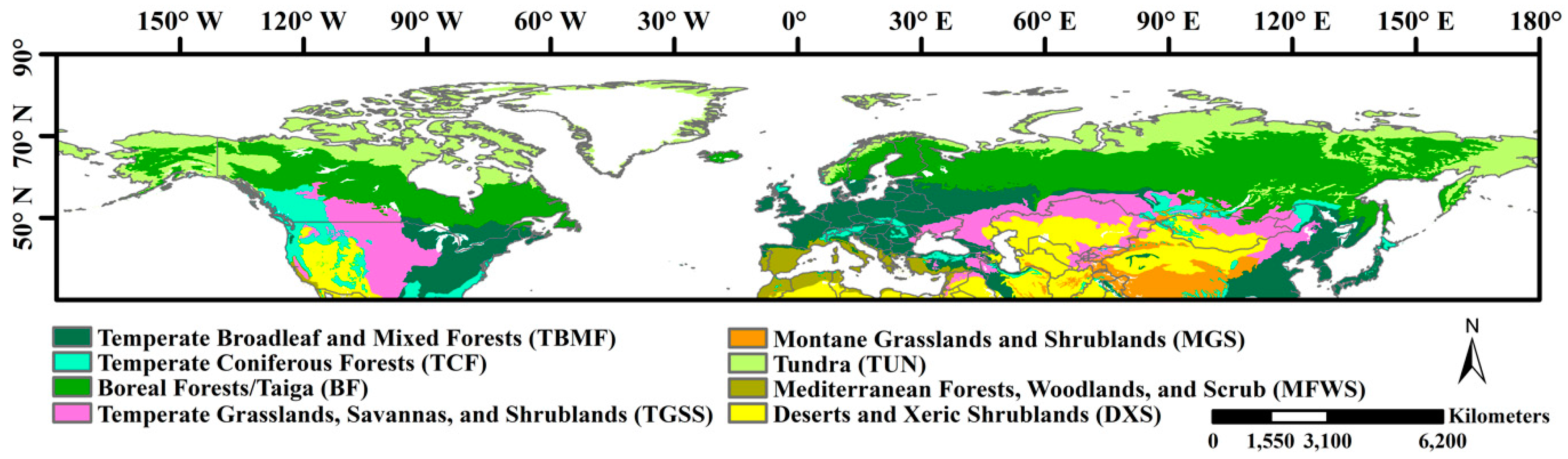
We concentrated our study on the northern hemisphere extratropical terrestrial ecosystems (>30° N; Figure 1) to estimate the phenology and further identify the growing season length because vegetation has evident seasonality in these areas. Previous studies have also concluded that satellite-derived NDVI for these regions have been less influenced by solar zenith angle effects [31,32]. To illuminate the drought variations at the biome level, we classified the vegetated areas into eight biomes according to the land cover classification map produced by Olson et al. [33]. To reduce the noise from nonvegetated areas, those areas with an annual mean NDVI of <0.1 were considered nonvegetated and were excluded from the remote sensing-based growing season length estimation.
2.2. Data Sets
2.2.1. Satellite NDVI Data Set
The NDVI has been widely used as an important proxy of photosynthetic activity to reflect the seasonality of vegetation. In this study, we used the 15-day GIMMS3g (third-generation Global Inventory Modeling and Mapping Studies) NDVI time series ranging from 1982 to 2015 to extract the dates of the SOS and EOS, and we subsequently identified the growing season length for each pixel. The GIMMS NDVI3g version1 was provided by the NASA Ames Ecological Forecasting Lab (http://ecocast.arc.nasa.gov/data/pub/gimms/3g.v1). Such NDVI3g data have a spatial resolution of 1/12° and have undergone rigorous correction, preprocessing, and validation, which has allowed the data to be widely used in previous climate change-related research [24,34].
2.2.2. Climate Data
Monthly precipitation and temperature data from 1982 to 2015 were obtained from the Climatic Research Unit Time Series (CRU-TS) data set (http://data.ceda.ac.uk/badc/cru/data/cru_ts). The latest version of this database, version 4.03, has been updated to span 1901 to 2018, with 0.5° spatial resolutions on land areas [35]. It was derived by the interpolation of monthly climate anomalies from extensive networks of weather station observations, and it has also been widely used in climate change-related studies [1,34].
2.2.3. SPEI Data
The SPEI data set for the period from 1901 to 2015, with a monthly frequency temporal resolution and a 0.5° spatial resolution at timescales from 1 to 48 months, was obtained from the Consejo Superior de Investigaciones Científicas (CSIC; http://spei.csic.es/database.html). The SPEI value at each pixel was calculated based on the difference between precipitation and potential evapotranspiration (PET) to describe the drought conditions with respect to normal conditions for a given period. This process revealed that a decrease in the SPEI may be caused by an abnormal increase in the PET or a decrease in precipitation. In this SPEI data set, the PET was calculated based on the FAO-56 (Food and Agriculture Organization of the United Nations, Irrigation and Drainage Paper 56) Penmann–Monteith equation [36], which integrates the mass transfer and energy balance and has been widely used around the world [5,7]. In addition, the SPEI has different implications at different timescales. For example, the SPEI for longer timescales, such as 12 or 24 months, can reflect medium-term trends in precipitation patterns and may provide an annual estimation of the reservoir levels, stream flows, and even groundwater levels. While for shorter timescales, such as 1 to 3 months, the SPEI can be used to mirror prompt changes in soil moisture, which is particularly important for biomass production. Because the aim of the study was to investigate the drought variations and their impacts on vegetation areas, which are sensitive to soil moisture, a 3-month timescale SPEI for the period of 1982 to 2015 was selected to reveal the variations in drought characteristics, including the drought duration, intensity, and frequency, during the growing season in the northern hemisphere.
2.2.4. Gross Primary Production Data
The 8-day interval-gridded gross primary production (GPP) data set from Global Land Surface Satellite (GLASS) products was used. This database covers 1982 to 2015 and globally has a 0.05° spatial resolution in vegetation areas. The GPP product was simulated from the integration of eight light-use efficiency models by the Bayesian model averaging method. Its accuracy has been validated by 155 flux sites around the world [37,38].
2.3. Estimation of the Growing Season Length from the NDVI
For each pixel, the length of the growing season was defined as the time interval between the SOS and EOS dates. To estimate the SOS and EOS from the NDVI data, we adopted the modified Savitzky–Golay filter to smooth out mutational noise in the NDVI time series that is generated by unstable atmospheric states, such as clouds [39]. Because various methods can be used to extract phenology dates from the NDVI time series, the estimated result of each method may be different. Therefore, to prevent the phenology estimation method from affecting the results, we selected four widely used methods to determine the SOS and EOS for the northern hemisphere.
For Method 1, we first used the double logistic method to fit the NDVI time series at a daily temporal resolution [24,34,40], and it can be described as:
where is the fitted NDVI at day ; is the initial background NDVI value; is the maximum NDVI value; and , , , and b are parameters of this function.
The annual variation curve of the NDVI was divided into two sections by the NDVI maximum value: the ascending part (indicating the vegetation recovery from the nongrowing season) in about the first half of the year and the descending part (indicating the process of plant senescence from the growing peak) in about the second half of the year. For the ascending part of the NDVI, the SOS date was extracted as the local maximum in the first derivative of the fitted NDVI, and for the latter part, the EOS date was extracted as the local minimum in the first derivative of the fitted NDVI. In other words, the date when the NDVI increased (or decreased) faster was determined as the SOS (or EOS).
In Method 2, the NDVI data were fitted with a double logistic function, and the second-order derivative of the fitted curve was then calculated. The two dates corresponding to the two local maximum points in the first half of the year were the SOS and the onset of maturity. The two dates corresponding to the two local maximum points in the second half of the year were the onset of senescence and the EOS [24].
In Methods 3 and 4, we also used the different threshold values method to extract the phenology. First, the NDVI data were fitted by the double logistic function shown in Equation (1). The fitted NDVI was then normalized by using the following function:
where NDVI represents the fitted daily NDVI data by the double logistic function; represents the minimum NDVI for each year, and represents the maximum NDVI for each year. In Method 3, the SOS was determined as the day when the increased to 0.2 in the spring, and the EOS was determined as the day when the decreased to 0.2 in the autumn. Method 4 was similar to Method 3, except that the threshold ratio value was set as 0.5. Finally, we used the average value of the four SOS and EOS extraction results as the final SOS and EOS applied in our study to reduce uncertainties caused by any single calculation algorithm.
2.4. Defining a Drought Event and the Drought Duration, Intensity, and Frequency
There are various drought indices that can be used to quantify the variations in drought characteristics, such as the Standardized Precipitation Index (SPI) proposed by McKee et al. [41], which is calculated based on precipitation data. The SPI has a wide application mainly because of its simplicity of calculation and because it can be calculated at different timescales to monitor droughts with respect to different usable water resources. However, it overlooked the effects of temperature and PET on the occurrence of drought events. Another widely used drought index, the Palmer Drought Severity Index (PDSI), which is calculated based on both precipitation and temperature data, as well as the water content of the soils, seems more appropriate for the objective and quantitative evaluation of drought severity in the context of global warming. However, because of its fixed temporal scale (yearly timescale), PDSI lacked the multiscale characteristic essential for us to determine the drought characteristics within a growing season period. Therefore, to verify the accuracy of the results of this paper, we analyzed the changes in drought characteristics by using the more accurate grid SPEI data, in which the PET was calculated by the Penman–Monteith equation [36]. Compared with the Thornthwaite method, the Penman–Monteith equation takes into account the combined effects of wind speed, radiation, and relative humidity on evapotranspiration; it was thus a more accurate, comprehensive, and physically based model for estimating the PET.
The monthly SPEI-3 (SPEI at a 3-month timescale) series for each pixel during the growing season from 1982 to 2015 was selected to construct the drought duration, intensity, and frequency maps. For example, for a specific pixel, the SOS occurred in March and the EOS occurred in November. The monthly SPEI series from March to November from 1982 to 2015 was then selected for the drought characteristic analysis. The drought event starts and end dates in the month were defined as when the SPEI fell below 0 and when the SPEI returned to a positive value, respectively. However, because the soil moisture can buffer vegetation growth during periods of moisture deficiency, in our analysis, a drought event was defined to occur when the SPEI value fell below 0 for at least three consecutive months. Once a drought event had been determined with its start and end months, the duration of the drought event was calculated by the number of months between the start (included) and end months (not included). In addition, the drought intensity was calculated as the value of the integral area between the SPEI line and the horizontal x axis (SPEI = 0) from the start to the end month of the drought, which indicated that the more negative the intensity value, the more severe the drought. The drought frequency was defined as the number of drought events that occurred over a defined period.
To compare the changes in drought duration and intensity before and after the critical time point of 1998, the total drought duration (TDD) and total drought intensity (TDI) were then calculated as the sum of the duration and intensity of the drought events that occurred in 1982–1998 and 1999–2015, respectively.
2.5. Statistical Analysis
The annual trends for climate factors, SPEI values, and drought characteristics were estimated by regressing them against the year over the periods of 1982–1998 and 1999–2015. To match the spatial resolution of the NDVI data, the precipitation, temperature, and GPP data were first resampled into 1/12° by using the bilinear interpolation method. The drought sensitivity of ecosystem production was determined based on a Pearson correlation analysis between the annual GPP and SPEI data, with high correlation coefficients indicating a high drought sensitivity (high vulnerability to drought) and vice versa [42]. The significance of correlations was evaluated at p < 0.05.
3. Results
3.1. Spatial Distribution of Averaged SOS and EOS from 1982 to 2015
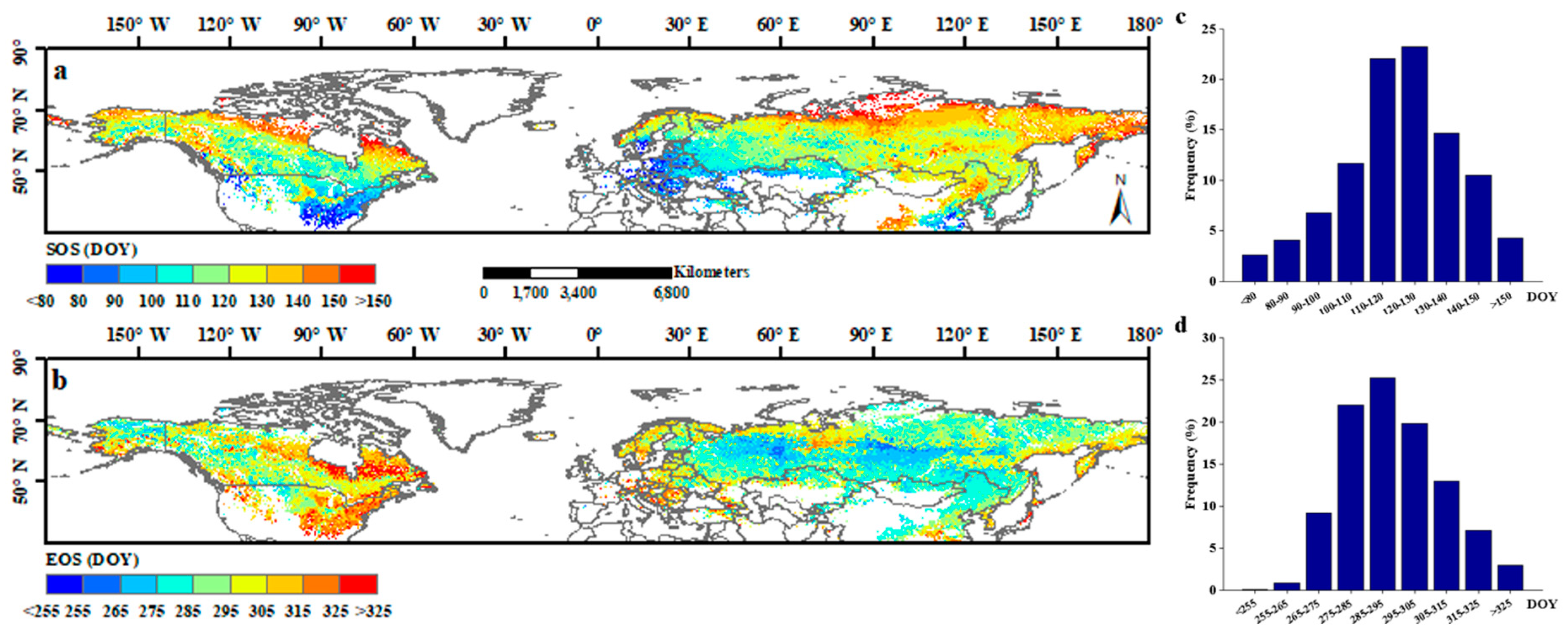
Spatial patterns of the SOS and EOS were shown in Figure 2. These results showed that the mean SOS in the 1982–2015 period in the northern hemisphere mainly occurred from March to May (from the 80th to 150th day of the year (DOY)), which accounted for 93.8% of the pixels (Figure 2c). Earlier SOS (<80th DOY) regions were located in the southeast regions of North America, the southwest regions of Eurasia, and the middle-east regions of China, whereas the later SOS (>150th DOY) regions were concentrated mainly in high-latitude areas (Figure 2a). Additionally, in more than 96.2% of the study area, the EOS occurred from September to November (from the 255th to 325th DOY), and 76.2% occurred from September to October (Figure 2d). Most late EOS (>315th DOY) regions were located in the southeastern and northeastern parts of North America and western Eurasia, whereas most early EOS (<275th DOY) regions were located in inner Asia (Figure 2b).
3.2. Temporal and Spatial Patterns of Climate Factors and SPEI within Vegetation Growing Seasons in 1982–1998 and 1999–2015
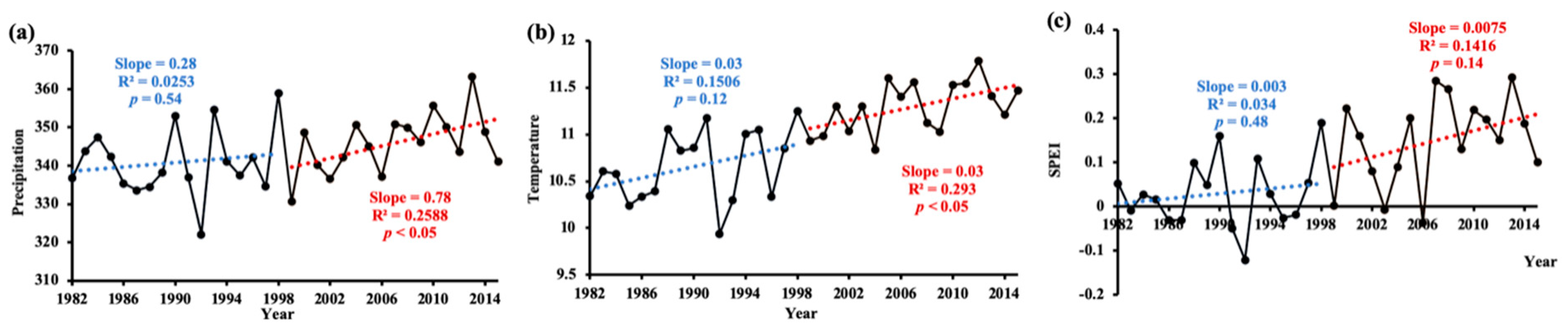
A piecewise linear regression method was used to quantify the change in annual averaged climate factors (mean value during the growing period), including precipitation and temperature before and after 1998. Results showed no obvious changing trend in precipitation in 1982–1998, but precipitation increased significantly (p < 0.05), by 7.8 mm per decade, in 1999–2015 (Figure 3a). With respect to temperature, no apparent warming hiatus was observed after 1998. On the contrary, the temperature increased by 0.3 °C per decade both before and after 1998, and this increasing trend was statistically significant (p < 0.05) in 1999–2015 (Figure 3b). In addition, it is worth noting that the standard deviation of precipitation and temperature were both higher in 1982–1998 than in 1999–2015. As for the SPEI, a significant (p < 0.01) increasing trend was observed over the entire study period, which indicated that the vegetation zone of the northern hemisphere had undergone a considerable wetting trend in the growing season of 1982–2015. When the period was divided into two parts, neither increasing trend in the SPEI was statistically significant, but the trend increased more rapidly in 1999–2015 (Figure 3c).
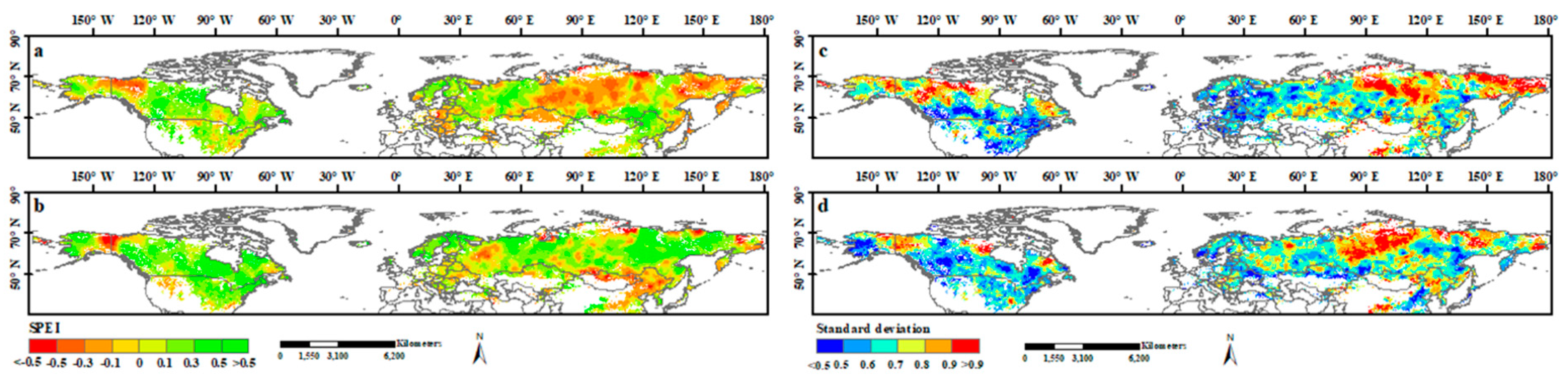
Spatial patterns of the SPEI during the two study periods were reflected by their mean values and the standard deviation. Significantly different spatial patterns in the mean SPEI were observed both before and after 1998 (Figure 4). In 1982–1998, the regions with a low SPEI (<−0.1) accounted for 27.7% of the study area and were mainly located in the high and mid-latitudes, including the middle and northeastern part of Russia, northwestern Canada, and northern Kazakhstan (Figure 4a). However, after 1998, the regions with a low SPEI decreased to 13.6% and were mainly concentrated in low-latitude areas, including northern Mongolia and northeastern China (Figure 4b). Overall, the high-latitude areas underwent a considerable increase in SPEI (wetting trend) in 1999–2015. Compared with the SPEI, the standard deviation also showed a high spatial heterogeneity for the study area, but no apparent difference was observed between the two study periods. Most standard deviations were in the range of 0.5 to 0.9. Regions with a high standard deviation were observed mainly in the northeastern and north-central parts of Russia and northwestern Canada, whereas areas with low standard deviations were widely concentrated in the middle- and low-latitude regions (Figure 4c,d).
3.3. Temporal and Spatial Patterns of Drought Characteristics in 1982–1998 and 1999–2015
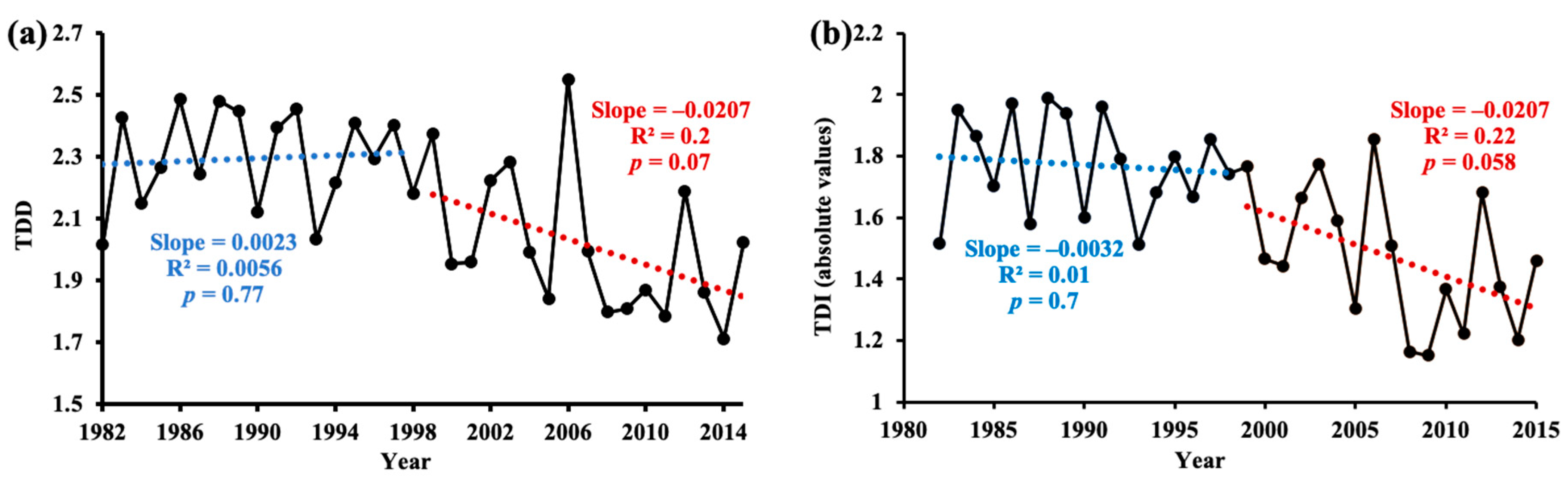
We observed that both the annual drought duration and drought intensity series changed abruptly at approximately 1998 across the entire period (Figure 5). Specifically, the drought duration showed a slight increasing trend before 1998, but this trend was subsequently reversed in 1999–2015, with a significantly (p < 0.1) decreasing trend by 2 months per decade (Figure 5a). The absolute values of drought intensity exhibited a slight decrease before 1998 but a strong decrease afterward, with a 6.5 times larger trend (Figure 5b).
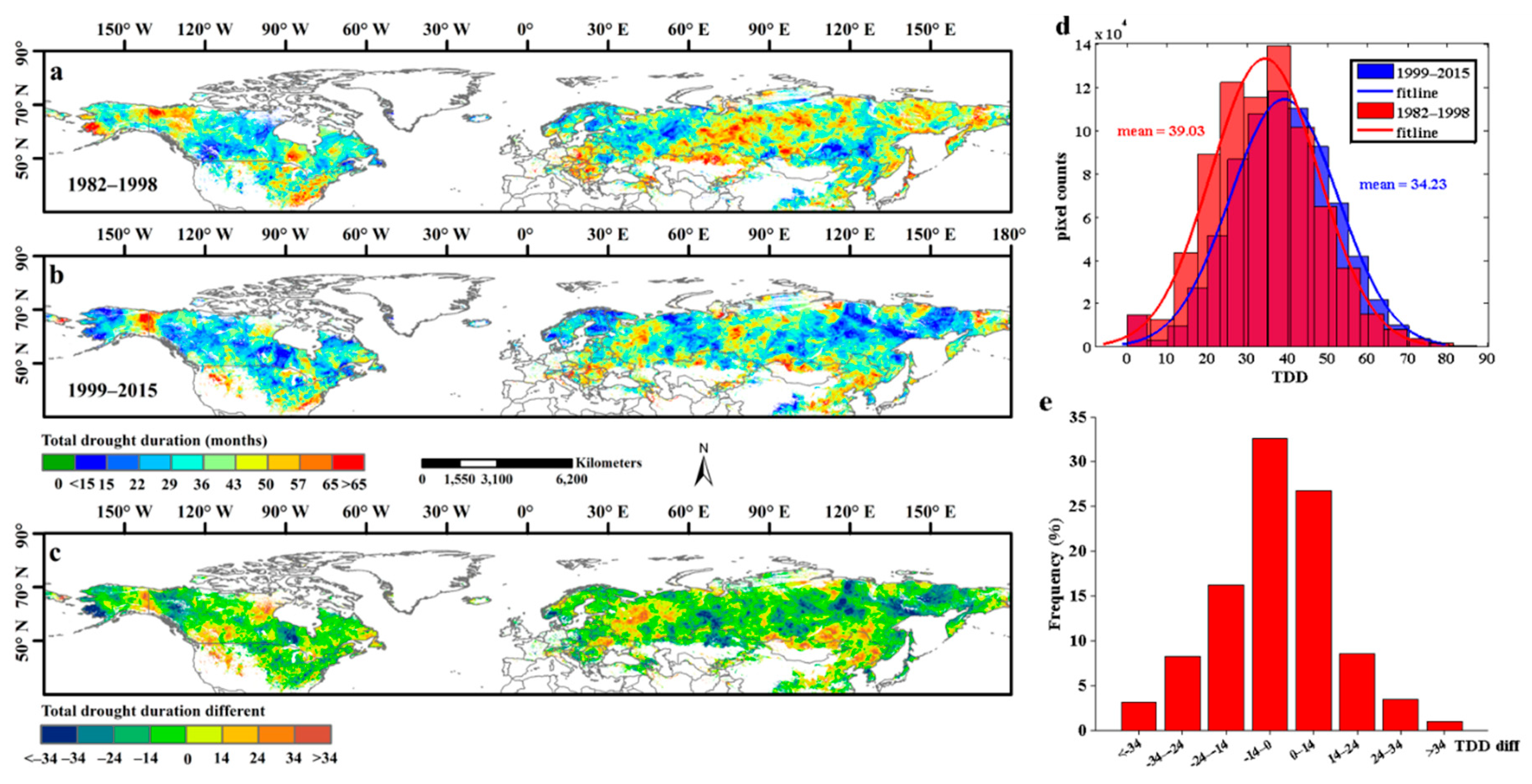
Figure 6 showed the TDD maps for each selected period (1982–1998 and 1999–2015). During the 1982–1998 period, more than 19.14% of the study areas had TDDs longer than 50 months, and these areas were located mainly in northwestern Canada, the eastern United States, northern Kazakhstan, and a large part of central and eastern Russia (Figure 6a). However, during the 1999–2015 period, the number of high-level TDD areas (TDD >50 months) decreased considerably and accounted for only about 11% of the study area. The high-level TDD areas in 1999–2015 were located mainly in intersection regions, such as North America and Canada, northern Inner Mongolia, eastern China, and scattered locations in Russia (Figure 6b). In addition, by calculating the difference in TDD between these two selected periods, we found that the percentage of TDD areas that had decreased accounted for 60.2% of the total study area, with more than 27.5% of the pixels showing a decrease of more than 14 months (Figure 6c,e). The distribution of these areas (TDD with a decrease of >14 months) closely coincided with the distribution of high-level TDD (>50 months) areas in 1982–1998 (Figure 6a,c). Overall, the mean TDD decreased from 39.03 months in 1982–1998 to 34.23 months in 1999–2015 (Figure 6d). However, we also found that about 13% of the pixels experienced a pronounced increase (>14 months) in TDD and that these areas were mainly located in low latitudes in the study area, such as northern Mongolia, northeastern China, and the eastern United States (Figure 6c,e).
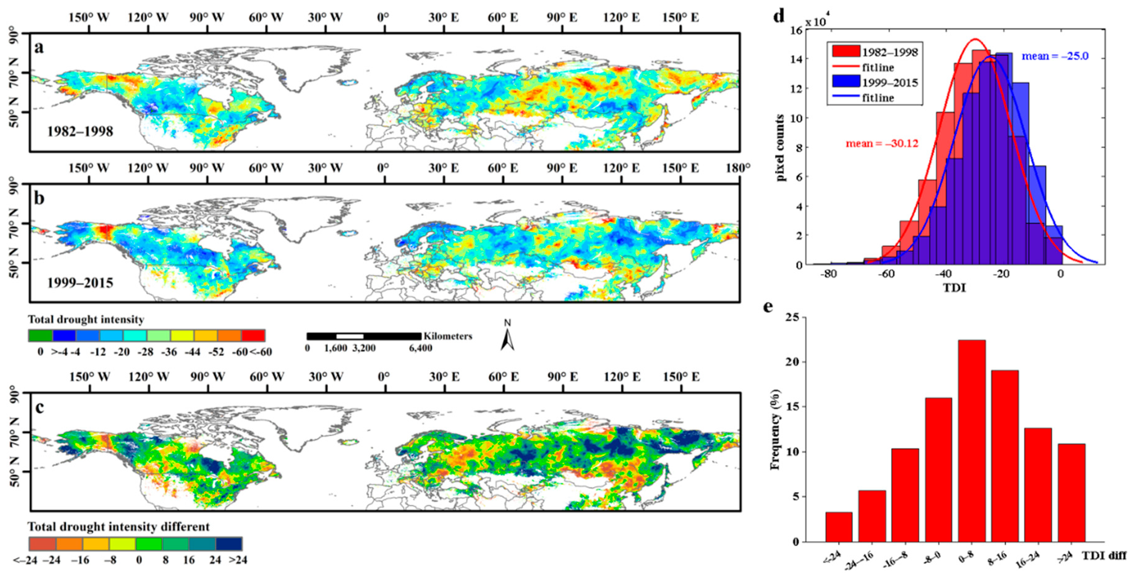
Differences in the TDI maps between the 1982–1998 and 1999–2015 periods were shown in Figure 7; the more negative the TDI value was, the more often the area was affected by high-severity droughts. The results showed that more than 64.8% of areas exhibited an increased TDI and that 23.5% of the pixels of the TDI increased by more than 16 (Figure 7c,e). In addition, it is worth noting that the mean TDI increased from −30.12 in 1982–1998 to −25.0 in 1999–2015 (Figure 7d), which further indicates that the effects of the drought were alleviated after 1998. Spatially, the TDI maps showed a roughly similar spatial pattern as the TDD during the two study periods because they are connected. The proportion of high-level drought intensity (TDI <−44) areas decreased from 13.2% in 1982–1998 to 6.7% in 1999–2015 in the study areas (Figure 7a,b), and these high-level drought intensity areas were concentrated mainly in eastern and middle Russia, northeastern China, and northern Kazakhstan during the 1999–2015 period.
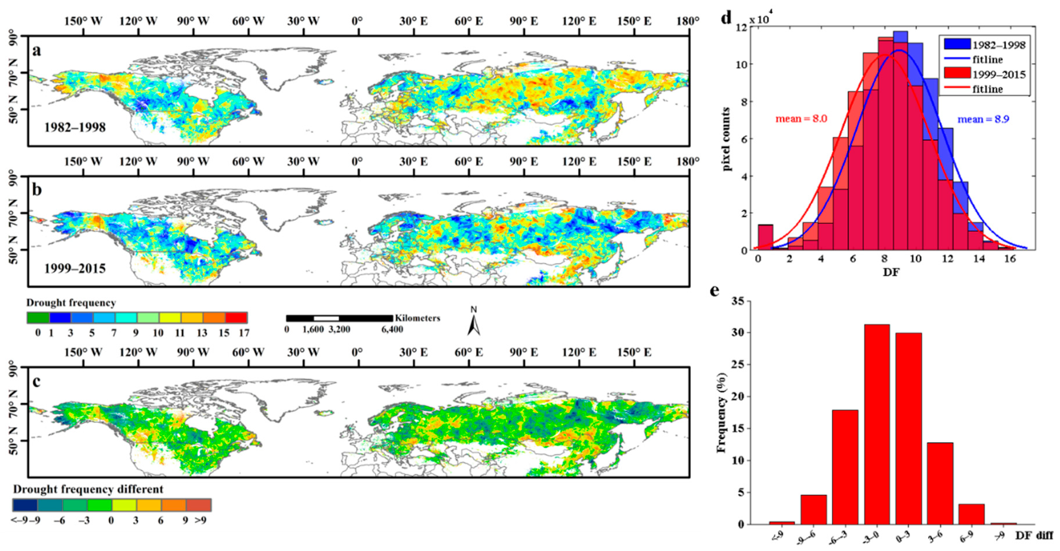
High drought frequency (>11 events) areas accounted for 16.1% of the study area in 1982–1998, and these areas were located mainly in northwestern Canada, northern Kazakhstan, and the central and eastern parts of Russia (Figure 8a). After 1998, the proportion of high drought frequency areas decreased significantly and accounted for only 9.6% of the total pixels. These high drought frequency areas in 1999–2015 were located mainly in northern Mongolia and northeastern China (Figure 8b). When comparing the drought frequency areas between the 1982–1998 and 1999–2015 periods, we found that 54.1% of the pixels showed a decrease in drought frequency and that 4.9% of them had decreased by more than 6 events (Figure 8c,e). Overall, the mean values for drought frequency decreased from 8.9 events in 1982–1998 to 8.0 events in 1999–2015 (Figure 8d). However, in a small proportion of areas, the drought frequency also showed a pronounced increase (>6 events), such as in Mongolia and northern China (Figure 8c).
3.4. Changes in TDD, TDI, and DF at the Biome Level
The mean TDD, TDI, and drought frequency at each biome during the 1982–1998 and 1999–2015 periods were presented in Figure 9. Results showed that the largest decrease in the mean TDD occurred in the tundra (TUN; decreased from 44.7 to 33.1 months) biome, followed by the boreal forests or taiga (BF; 39.3 to 31.2 months), temperate coniferous forests (TCF; 37.9 to 31.9 months), temperate grasslands, savannas, and shrublands (TGSS; 37.6 to 33.9 months), and montane grasslands and shrublands (MGS; 39.8 to 36.6 months) biomes, whereas the deserts and xeric shrublands (DXS), temperate broadleaf and mixed forests (TBMF), and Mediterranean forests, woodlands, and scrub (MFWS) biomes showed no obvious change (Figure 9a). At the same time, except for MFWS, all the biomes presented increased in TDI (Figure 9b). The increased amplitudes of each biome were roughly consistent with the changes in TDD, whereas the largest increase in TDI also occurred in the TUN (−35.5 to −25.8) biome, followed by the BF (−32.0 to −23.1), TCF (−29.2 to −22.8), TGSS (−27.2 to −23.5), and MGS (−29.8 to −26.3) biomes. As for the changes in mean drought frequency (DF), only the TUN, BF, and TCF biomes exhibited obvious decreases, from 9.9 to 7.9, 9.3 to 7.6, and 8.7 to 7.4, respectively (Figure 9c).
As regard to the interannual variations in mean drought duration and drought intensity during the two study periods among different biomes (Table 1), we found that the annual trend for drought duration had transformed from increasing to decreasing trend in the TBMF, TCF, and TGSS biomes. Among them, the trend in the TCF biome decreased significantly (p < 0.05) by 0.06 months per year during the 1999–2015 period. In the TUN biome, the drought duration exhibited a slight decrease before 1998, but it increased more strongly afterward, with an 18 times larger trend. The drought intensity showed nonsignificant trends in the TBMF, TCF, TGSS, MGS, MFWS, DXS, and TUN biomes in 1982–1998, but a significant increase afterward in the TCF (p < 0.05) and TUN (p < 0.01) biomes. In addition, the drought intensity increased significantly (p < 0.05) in the BF biome before 1998, but this trend was subsequently stalled.
3.5. The Sensitivity of Ecosystem Production to Drought
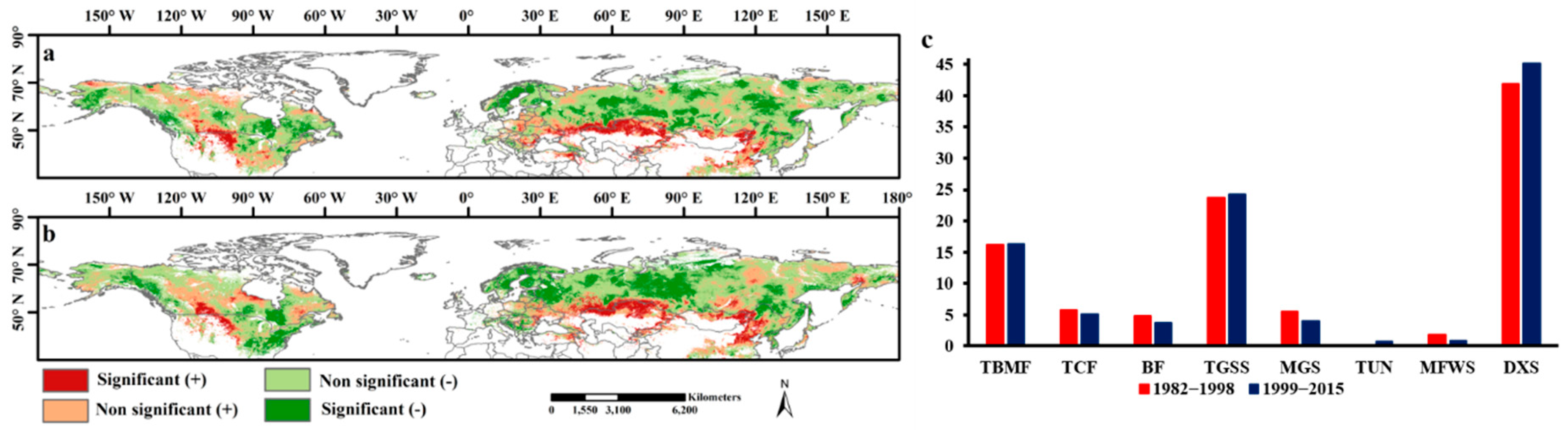
The sensitivity of ecosystem production to drought was reflected in the ability of vegetation to respond to and recover from the impacts of a drought event. This was a particularly important indicator when estimating the drought impacts. Drought that occurs in highly drought-sensitive areas will cause a larger reduction in production than will drought in low drought-sensitive areas. Our results showed that the interannual variation in GPP was closely correlated with the annual SPEI (averaged values during the growing season) in most of the study areas (Figure 10a,b), which indicated that the dryness or wetness exerts a large influence on the GPP. The spatial patterns of highly drought-sensitive areas were roughly the same over the two study periods, and they were located mainly in arid and semi-arid areas, such as northern Kazakhstan, northern Mongolia, northern China, and the midwestern part of the United States. It is worth noting that at the biome level, a great proportion of the highly drought-sensitive areas were concentrated in the DXS (43.5%), TGSS (24%), and TBMF (16.3%) biomes (Figure 10c), where the drought duration, intensity, and frequency were not significantly alleviated in 1999–2015. However, the proportion of highly drought-sensitive areas in biomes with significant drought relief was very small. For example, these proportions were only 0.44% (averaged across the two study periods) and 5.4% of the highly drought-sensitive areas were located in the TUN and TCF biomes, respectively. This means that even though the average number of the occurrence of drought events was reduced over the vegetation zone of the northern hemisphere, the mismatch between the reduction in drought areas and the highly drought-sensitive areas still makes the impact of drought on vegetation nonnegligible.
4. Discussion
Temperature, precipitation, and PET are three key variables of the SPEI that can greatly influence the variations in drought. Temperatures have increased significantly around the world in recent decades, and the predominant explanations given have been the increasing use of fossil fuels and the increase in greenhouse gas emissions caused by anthropogenic activities [43,44]. In this context, recent work suggests that global aridity has increased in step with the observed warming trends and that this drying will aggravate for many regions as the continuous rise in temperature further increases evapotranspiration [7,18]. However, in contrast to the general expectation that a warmer climate will bring about an increase in PET, several studies have demonstrated that the PET has shown a steady downward trend over the last 18–20 years, both globally [45] and regionally in many areas of the northern hemisphere, such as in northern China [46], India [47], Italy [48], and Canada [49]. This is known as the “evaporation paradox” phenomenon [50]. Recently, several studies have attempted to explain what causes this paradoxical phenomenon. Some authors have concluded that under the backdrop of climate change, a weakening of PET resulted from the combined effects of sunshine hours, wind speed, solar radiation, and relative humidity overcomes the increase in PET induced by the temperature elevation and eventually results in increased PET in some regions [51]. It is important to note that a regional study in China emphasized that the rising temperatures contribute to a very limited extent to the variation in PET compared with other climate factors [52]. Our study results supported the view that using only temperature as input data to estimate the variation in PET, such as by using the Thornthwaite method [53], will overestimate the effects of global warming and eventually result in producing incorrect drought trends [1,5]. This may partially explain why recently published studies have generally produced apparently conflicting results regarding to drought trends in the context of climate change.
In addition, a great deal of research has indicated that human-influenced global warming not only affects evapotranspiration but may also be partly responsible for increases in heavy precipitation [54,55]. Our results revealed a significant increase in precipitation in the vegetation zone of the northern hemisphere (Figure 3a) and showed that the areas with a wetting trend in 1999–2015 were located mainly in the high and mid-latitudes (Figure 4), which is consistent with the result by Zhang et al. [56]. That study also attributed the significant increases in precipitation in the mid-latitudes of the northern hemisphere to anthropogenic forcing [56]. The wetting trend in high latitudes was also identified by Zhang et al. [57], but they contributed this wetting trend (especially for Eurasian Arctic regions) to the enhancement of poleward atmospheric moisture transport. In parallel, Spinoni et al. [58] investigated the drought characteristics variations globally based on SPI and also revealed that the drought frequency decreased significantly in Northern Hemisphere in recent decades. Contrary to our results, however, they concluded that the drought duration and intensity have changed insignificantly. The main reason for this discrepancy was that the SPI calculation was based only on precipitation data, and the effects of temperature and PET on drought were overlooked. Guan et al. [59] used AI and Palmer Drought Severity Index (PDSI) to study the response of drought to the recent global warming hiatus in Northern Hemisphere and also revealed a wetting trend over the mid-to-high latitudes. However, they deduced that the wetting zone (high latitudes of Northern Hemisphere) is likely to disappear when the temporary global warming hiatus ended. In other words, they attributed this wetting trend to the slowdown of the increase in temperature.
However, contrary to the prevailing view of a warming hiatus after 1998 that occurred in both the global and hemispheric scale [59], our results showed that increasing trends in the growing season temperatures of Northern Hemisphere during this time period were even more statistically significant than those before. This discrepancy indicated that the reversed trend (decreasing trend) in non-growing season temperature may have overweighed the increasing trend in growing season temperature and eventually resulted in slowing down of rising in annual mean temperature in the Northern Hemisphere. However, such assumption needs to be further validated by future work. In addition, the increase in growing season temperature may be related to the snow-albedo feedback because a rapid rise in temperatures will accelerate the melting of snow, which in turn will reduce the surface albedo in high-altitude areas of the northern hemisphere, resulting in enhanced absorption of solar radiation on the land surface and further increasing the temperature [60]. Beyond that, the accelerated melting of the snow and ice may be another important reason (besides the increase in precipitation) of why the areas with wetting trends are located mainly in the high latitudes. In addition, drought events primarily affect the productivity of the vegetation. However, an interesting phenomenon is that the significantly increasing trend in production before 1998 (referred to by the GPP and NDVI) was slowed or even reversed during the 1999–2015 period in a great part of the northern hemisphere, while the drought events obviously decreased. Yuan et al. [61] tried to explain the slowing down or even the decreased in vegetation production during this period in terms of an increased atmospheric vapor pressure deficit, which describes the difference between the water vapor pressure at saturation and the actual water vapor pressure for a given temperature, and plays a critical role in determining plant photosynthesis. Those authors concluded that the increased vapor pressure deficit had offset the positive CO2 fertilization effect in 1999–2015 and eventually resulted in persistent and widespread decreases in vegetation productivity. However, our results revealed that the mismatch between the distribution of highly drought-vulnerable areas and significant decreases in the areas of drought may also be partly responsible for this discrepancy.
Regarding the method, we suggest that the drought indices should preferentially include the dynamics of temperature in the context of global warming. Therefore, we selected SPEI, which combines the sensitivity of the PDSI with changes in the evaporation demand (mainly caused by temperature fluctuations and trends) and the multitemporal nature of the SPI, to define the drought events. In this context, our findings of a significant wetting trend within the growing season in the northern hemisphere should be more consistent with the real-life situation. Additionally, compared with the change in drought as characterized by area [62], our study used the drought duration, intensity, and frequency, which could comprehensively express the occurrence of drought within a time interval and had better applicability in the severity analysis method. Despite these achievements, this study still faced two limitations. First, because of the limited availability of data, we did not show the temporal and spatial variations in PET, which were also important to fully understand the climatic drivers in regional drought. Second, we used only CRU-TS temperature data to reveal changes in temperature within the growing season in vegetation areas of the northern hemisphere. However, several recent authors have emphasized that other important aspects of the warming hiatus were related to observational biases in global surface temperature data that could well have muted the recent warming [63,64]. Therefore, cross-validation of our comparison with different data sets would seem to be particularly necessary.
5. Conclusions
Using various high-quality data sets, namely, the GIMMS-3g 1/12° spatial resolution NDVI, CRU-TS climate (0.05°), and SPEI (0.05°), we analyzed the variation in drought characteristics, including the drought duration, intensity, and frequency, within the growing season in the northern hemisphere before and after the important time point of 1998, after which the global warming trend was stalled. Furthermore, on the basis of these analyses, we explored the impacts of the spatiotemporal variation in drought characteristics on various vegetation types. The results indicated that the annual growing season precipitation, temperature, and SPEI all showed significant (p > 0.05) increases during the 1982–2015 period and that the increasing trend in temperature after 1998 was steadier and more significant than before. No obvious changes in drought characteristics were observed before 1998, but afterward, both the drought duration, drought frequency, and absolute values of drought intensity decreased significantly. Spatially, the areas with considerable wetting trend were located mainly at high latitudes, such as in northwestern Canada, the eastern United States, and a great part of central and eastern Russia. At the biome level, significant decreases in drought characteristics mainly occurred in the TUN, BF, and TCF biomes. In addition, to fully understand the potential damage to vegetation from drought, we extracted the highly drought-vulnerable areas by examining the correlation between GPP and the SPEI. We found that the highly drought-vulnerable areas were located mainly in the low latitudes and that they mainly occurred in the DXS, TGSS, and TBMF biomes, which is inconsistent with the distribution of obvious decrease in drought areas. Therefore, we suggested that although overall wetting trends were found in vegetation areas in the northern hemisphere, the low latitudes (especially the arid and semi-arid areas) still face a greater threat of drought.
Author Contributions
Z.Z. and W.W. designed the research and performed the analysis, and Z.Z. wrote the first draft. Z.Z., Y.L., W.W., Y.Z., Z.L., and X.W. reviewed and edited the draft. Z.Z. and H.H. collected the data. All authors have read and agreed to the published version of the manuscript.
Funding
This research was funded by the Strategic Priority Research Program of the Chinese Academy of Sciences (XDA19040101, XDA19040304).
Conflicts of Interest
The authors declare no conflict of interest.
References
- Trenberth, K.E.; Dai, A.; Van Der Schrier, G.; Jones, P.D.; Barichivich, J.; Briffa, K.R.; Sheffield, J. Global warming and changes in drought. Nat. Clim. Chang. 2014, 4, 17–22. [Google Scholar] [CrossRef]
- Vicente-Serrano, S.M.; Gouveia, C.; Camarero, J.J.; Beguería, S.; Trigo, R.; López-Moreno, J.I.; Azorín-Molina, C.; Pasho, E.; Lorenzo-Lacruz, J.; Revuelto, J. Response of vegetation to drought time-scales across global land biomes. Proc. Natl. Acad. Sci. USA 2013, 110, 52–57. [Google Scholar] [CrossRef] [PubMed] [Green Version]
- Cook, E.R.; Seager, R.; Cane, M.A.; Stahle, D.W. North American drought: Reconstructions, causes, and consequences. Earth-Sci. Rev. 2007, 81, 93–134. [Google Scholar] [CrossRef]
- Sternberg, T. Regional drought has a global impact. Nature 2011, 472, 169. [Google Scholar] [CrossRef]
- Sheffield, J.; Wood, E.F.; Roderick, M.L. Little change in global drought over the past 60 years. Nature 2012, 491, 435–438. [Google Scholar] [CrossRef]
- Samaniego, L.; Thober, S.; Kumar, R.; Wanders, N.; Rakovec, O.; Pan, M.; Zink, M.; Sheffield, J.; Wood, E.F.; Marx, A. Anthropogenic warming exacerbates European soil moisture droughts. Nat. Clim. Chang. 2018, 8, 421. [Google Scholar] [CrossRef]
- Dai, A. Increasing drought under global warming in observations and models. Nat. Clim. Chang. 2013, 3, 52–58. [Google Scholar] [CrossRef]
- Cai, W.; Cowan, T.; Briggs, P.; Raupach, M. Rising temperature depletes soil moisture and exacerbates severe drought conditions across southeast Australia. Geophys. Res. Lett. 2009, 36. [Google Scholar] [CrossRef]
- Xu, K.; Yang, D.; Yang, H.; Li, Z.; Qin, Y.; Shen, Y. Spatio-temporal variation of drought in China during 1961–2012: A climatic perspective. J. Hydrol. 2015, 526, 253–264. [Google Scholar] [CrossRef]
- Zhao, M.; Running, S.W. Drought-induced reduction in global terrestrial net primary production from 2000 through 2009. Science 2010, 329, 940–943. [Google Scholar] [CrossRef] [Green Version]
- Stocker, B.D.; Zscheischler, J.; Keenan, T.F.; Prentice, I.C.; Seneviratne, S.I.; Peñuelas, J. Drought impacts on terrestrial primary production underestimated by satellite monitoring. Nat. Geosci. 2019, 12, 264–270. [Google Scholar] [CrossRef]
- Adams, H.D.; Zeppel, M.J.; Anderegg, W.R.; Hartmann, H.; Landhäusser, S.M.; Tissue, D.T.; Huxman, T.E.; Hudson, P.J.; Franz, T.E.; Allen, C.D. A multi-species synthesis of physiological mechanisms in drought-induced tree mortality. Nat. Ecol. Evol. 2017, 1, 1285–1291. [Google Scholar] [CrossRef]
- Engelbrecht, B.M.; Comita, L.S.; Condit, R.; Kursar, T.A.; Tyree, M.T.; Turner, B.L.; Hubbell, S.P. Drought sensitivity shapes species distribution patterns in tropical forests. Nature 2007, 447, 80–82. [Google Scholar] [CrossRef] [PubMed]
- Hänke, H.; Börjeson, L.; Hylander, K.; Enfors-Kautsky, E. Drought tolerant species dominate as rainfall and tree cover returns in the West African Sahel. Land Use Policy 2016, 59, 111–120. [Google Scholar] [CrossRef] [Green Version]
- Zhang, X.; Chen, N.; Li, J.; Chen, Z.; Niyogi, D. Multi-sensor integrated framework and index for agricultural drought monitoring. Remote Sens. Environ. 2017, 188, 141–163. [Google Scholar] [CrossRef] [Green Version]
- Peng, J.; Wu, C.; Zhang, X.; Wang, X.; Gonsamo, A. Satellite detection of cumulative and lagged effects of drought on autumn leaf senescence over the Northern Hemisphere. Glob. Chang. Biol. 2019, 25, 2174–2188. [Google Scholar] [CrossRef]
- Ivits, E.; Horion, S.; Erhard, M.; Fensholt, R. Assessing European ecosystem stability to drought in the vegetation growing season. Glob. Ecol. Biogeogr. 2016, 25, 1131–1143. [Google Scholar] [CrossRef]
- Cook, B.I.; Smerdon, J.E.; Seager, R.; Coats, S. Global warming and 21 st century drying. Clim. Dyn. 2014, 43, 2607–2627. [Google Scholar] [CrossRef] [Green Version]
- Stocker, T.F.; Qin, D.; Plattner, G.-K.; Tignor, M.; Allen, S.K.; Boschung, J.; Nauels, A.; Xia, Y.; Bex, V.; Midgley, P.M. Climate change 2013: The physical science basis. In Contribution of Working Group I to the Fifth Assessment Report of the Intergovernmental Panel on Climate Change; Cambridge University Press: New York, NY, USA, 2013; Volume 1535. [Google Scholar]
- Kosaka, Y.; Xie, S.-P. Recent global-warming hiatus tied to equatorial Pacific surface cooling. Nature 2013, 501, 403–407. [Google Scholar] [CrossRef] [Green Version]
- Wu, H.T.J.; Lau, W.K.M. Detecting climate signals in precipitation extremes from TRMM (1998–2013)—Increasing contrast between wet and dry extremes during the “global warming hiatus”. Geophys. Res. Lett. 2016, 43, 1340–1348. [Google Scholar] [CrossRef]
- Wang, L.; Yuan, X.; Xie, Z.; Wu, P.; Li, Y. Increasing flash droughts over China during the recent global warming hiatus. Sci. Rep. 2016, 6, 30571. [Google Scholar] [CrossRef] [PubMed]
- Ballantyne, A.; Smith, W.; Anderegg, W.; Kauppi, P.; Sarmiento, J.; Tans, P.; Shevliakova, E.; Pan, Y.; Poulter, B.; Anav, A. Accelerating net terrestrial carbon uptake during the warming hiatus due to reduced respiration. Nat. Clim. Chang. 2017, 7, 148–152. [Google Scholar] [CrossRef]
- Wang, X.; Xiao, J.; Li, X.; Cheng, G.; Ma, M.; Zhu, G.; Arain, M.A.; Black, T.A.; Jassal, R.S. No trends in spring and autumn phenology during the global warming hiatus. Nat. Commun. 2019, 10, 1–10. [Google Scholar] [CrossRef] [PubMed]
- Huber, M.; Knutti, R. Natural variability, radiative forcing and climate response in the recent hiatus reconciled. Nat. Geosci. 2014, 7, 651–656. [Google Scholar] [CrossRef]
- Douville, H.; Voldoire, A.; Geoffroy, O. The recent global warming hiatus: What is the role of Pacific variability? Geophys. Res. Lett. 2015, 42, 880–888. [Google Scholar] [CrossRef]
- England, M.H.; McGregor, S.; Spence, P.; Meehl, G.A.; Timmermann, A.; Cai, W.; Gupta, A.S.; McPhaden, M.J.; Purich, A.; Santoso, A. Recent intensification of wind-driven circulation in the Pacific and the ongoing warming hiatus. Nat. Clim. Chang. 2014, 4, 222–227. [Google Scholar] [CrossRef]
- Santer, B.D.; Bonfils, C.; Painter, J.F.; Zelinka, M.D.; Mears, C.; Solomon, S.; Schmidt, G.A.; Fyfe, J.C.; Cole, J.N.; Nazarenko, L. Volcanic contribution to decadal changes in tropospheric temperature. Nat. Geosci. 2014, 7, 185–189. [Google Scholar] [CrossRef] [Green Version]
- Li, C.; Stevens, B.; Marotzke, J. Eurasian winter cooling in the warming hiatus of 1998–2012. Geophys. Res. Lett. 2015, 42, 8131–8139. [Google Scholar] [CrossRef] [Green Version]
- Trenberth, K.E.; Fasullo, J.T.; Branstator, G.; Phillips, A.S. Seasonal aspects of the recent pause in surface warming. Nat. Clim. Chang. 2014, 4, 911–916. [Google Scholar] [CrossRef] [Green Version]
- Piao, S.; Cui, M.; Chen, A.; Wang, X.; Ciais, P.; Liu, J.; Tang, Y. Altitude and temperature dependence of change in the spring vegetation green-up date from 1982 to 2006 in the Qinghai-Xizang Plateau. Agric. For. Meteorol. 2011, 151, 1599–1608. [Google Scholar] [CrossRef]
- Yang, Y.; Guan, H.; Shen, M.; Liang, W.; Jiang, L. Changes in autumn vegetation dormancy onset date and the climate controls across temperate ecosystems in China from 1982 to 2010. Glob. Chang. Biol. 2015, 21, 652–665. [Google Scholar] [CrossRef] [PubMed]
- Olson, D.M.; Dinerstein, E.; Wikramanayake, E.D.; Burgess, N.D.; Powell, G.V.; Underwood, E.C.; D’amico, J.A.; Itoua, I.; Strand, H.E.; Morrison, J.C. Terrestrial Ecoregions of the World: A New Map of Life on EarthA new global map of terrestrial ecoregions provides an innovative tool for conserving biodiversity. BioScience 2001, 51, 933–938. [Google Scholar] [CrossRef]
- Wu, C.; Wang, X.; Wang, H.; Ciais, P.; Peñuelas, J.; Myneni, R.B.; Desai, A.R.; Gough, C.M.; Gonsamo, A.; Black, A.T. Contrasting responses of autumn-leaf senescence to daytime and night-time warming. Nat. Clim. Chang. 2018, 8, 1092–1096. [Google Scholar] [CrossRef] [Green Version]
- Harris, I.; Osborn, T.J.; Jones, P.; Lister, D. Version 4 of the CRU TS monthly high-resolution gridded multivariate climate dataset. Sci. Data 2020, 7, 1–18. [Google Scholar] [CrossRef] [PubMed] [Green Version]
- Allen, R.G.; Pereira, L.S.; Raes, D.; Smith, M. Crop Evapotranspiration-Guidelines for Computing Crop Water Requirements-FAO Irrigation and Drainage Paper 56; FAO: Rome, Italy, 1998; Volume 300, p. D05109. [Google Scholar]
- Wang, X.; Wu, C. Estimating the peak of growing season (POS) of China’s terrestrial ecosystems. Agric. For. Meteorol. 2019, 278, 107639. [Google Scholar] [CrossRef]
- Yuan, W.; Liu, S.; Yu, G.; Bonnefond, J.-M.; Chen, J.; Davis, K.; Desai, A.R.; Goldstein, A.H.; Gianelle, D.; Rossi, F. Global estimates of evapotranspiration and gross primary production based on MODIS and global meteorology data. Remote Sens. Environ. 2010, 114, 1416–1431. [Google Scholar] [CrossRef] [Green Version]
- Chen, J.; Jönsson, P.; Tamura, M.; Gu, Z.; Matsushita, B.; Eklundh, L. A simple method for reconstructing a high-quality NDVI time-series data set based on the Savitzky–Golay filter. Remote Sens. Environ. 2004, 91, 332–344. [Google Scholar] [CrossRef]
- Liu, Q.; Fu, Y.H.; Zhu, Z.; Liu, Y.; Liu, Z.; Huang, M.; Janssens, I.A.; Piao, S. Delayed autumn phenology in the Northern Hemisphere is related to change in both climate and spring phenology. Glob. Chang. Biol. 2016, 22, 3702–3711. [Google Scholar] [CrossRef]
- McKee, T.B.; Doesken, N.J.; Kleist, J. The relationship of drought frequency and duration to time scales. In Proceedings of the 8th Conference on Applied Climatology, Anaheim, CA, USA, 17–22 January 1993; pp. 179–183. [Google Scholar]
- Wang, H.; He, B.; Zhang, Y.; Huang, L.; Chen, Z.; Liu, J. Response of ecosystem productivity to dry/wet conditions indicated by different drought indices. Sci. Total Environ. 2018, 612, 347–357. [Google Scholar] [CrossRef]
- Gleckler, P.J.; Santer, B.; Domingues, C.; Pierce, D.; Barnett, T.; Church, J.; Taylor, K.; AchutaRao, K.; Boyer, T.; Ishii, M. Human-induced global ocean warming on multidecadal timescales. Nat. Clim. Chang. 2012, 2, 524–529. [Google Scholar] [CrossRef]
- Kerr, R.A. It’s Official: Humans Are behind Most of Global Warming; American Association for the Advancement of Science: Washington, DC, USA, 2001. [Google Scholar]
- Roderick, M.L.; Farquhar, G.D. The cause of decreased pan evaporation over the past 50 years. Science 2002, 298, 1410–1411. [Google Scholar] [PubMed]
- Han, J.; Wang, J.; Zhao, Y.; Wang, Q.; Zhang, B.; Li, H.; Zhai, J. Spatio-temporal variation of potential evapotranspiration and climatic drivers in the Jing-Jin-Ji region, North China. Agric. For. Meteorol. 2018, 256, 75–83. [Google Scholar] [CrossRef]
- Bandyopadhyay, A.; Bhadra, A.; Raghuwanshi, N.; Singh, R. Temporal trends in estimates of reference evapotranspiration over India. J. Hydrol. Eng. 2009, 14, 508–515. [Google Scholar] [CrossRef]
- Moonen, A.; Ercoli, L.; Mariotti, M.; Masoni, A. Climate change in Italy indicated by agrometeorological indices over 122 years. Agric. For. Meteorol. 2002, 111, 13–27. [Google Scholar] [CrossRef]
- Burn, D.H.; Hesch, N.M. Trends in evaporation for the Canadian Prairies. J. Hydrol. 2007, 336, 61–73. [Google Scholar] [CrossRef]
- Peterson, T.C.; Golubev, V.S.; Groisman, P.Y. Evaporation losing its strength. Nature 1995, 377, 687–688. [Google Scholar] [CrossRef]
- Wang, Q.; Wang, J.; Zhao, Y.; Li, H.; Zhai, J.; Yu, Z.; Zhang, S. Reference evapotranspiration trends from 1980 to 2012 and their attribution to meteorological drivers in the three-river source region, China. Int. J. Climatol. 2016, 36, 3759–3769. [Google Scholar] [CrossRef]
- Gao, G.; Chen, D.; Ren, G.; Chen, Y.; Liao, Y. Spatial and temporal variations and controlling factors of potential evapotranspiration in China: 1956–2000. J. Geogr. Sci. 2006, 16, 3–12. [Google Scholar] [CrossRef]
- Thornthwaite, C.W. An approach toward a rational classification of climate. Geogr. Rev. 1948, 38, 55–94. [Google Scholar] [CrossRef]
- Min, S.K.; Zhang, X.; Zwiers, F.W.; Hegerl, G.C. Human contribution to more-intense precipitation extremes. Nature 2011, 470, 378–381. [Google Scholar] [CrossRef] [PubMed]
- Groisman, P.Y.; Knight, R.W.; Easterling, D.R.; Karl, T.R.; Hegerl, G.C.; Razuvaev, V.A.N. Trends in intense precipitation in the climate record. J. Clim. 2005, 18, 1326–1350. [Google Scholar] [CrossRef]
- Zhang, X.; Zwiers, F.W.; Hegerl, G.C.; Lambert, F.H.; Gillett, N.P.; Solomon, S.; Stott, P.A.; Nozawa, T. Detection of human influence on twentieth-century precipitation trends. Nature 2007, 448, 461–465. [Google Scholar] [CrossRef] [PubMed]
- Zhang, X.; He, J.; Zhang, J.; Polyakov, I.; Gerdes, R.; Inoue, J.; Wu, P. Enhanced poleward moisture transport and amplified northern high-latitude wetting trend. Nat. Clim. Chang. 2013, 3, 47–51. [Google Scholar] [CrossRef]
- Spinoni, J.; Naumann, G.; Carrao, H.; Barbosa, P.; Vogt, J. World drought frequency, duration, and severity for 1951–2010. Int. J. Climatol. 2014, 34, 2792–2804. [Google Scholar] [CrossRef] [Green Version]
- Guan, X.; Huang, J.; Guo, R. Changes in aridity in response to the global warming hiatus. J. Meteorol. Res. 2017, 31, 117–125. [Google Scholar] [CrossRef]
- Hall, A.; Qu, X. Using the current seasonal cycle to constrain snow albedo feedback in future climate change. Geophys. Res. Lett. 2006, 33. [Google Scholar] [CrossRef] [Green Version]
- Yuan, W.; Zheng, Y.; Piao, S.; Ciais, P.; Lombardozzi, D.; Wang, Y.; Ryu, Y.; Chen, G.; Dong, W.; Hu, Z.; et al. Increased atmospheric vapor pressure deficit reduces global vegetation growth. Sci. Adv. 2019, 5. [Google Scholar] [CrossRef] [Green Version]
- Tong, S.; Lai, Q.; Zhang, J.; Bao, Y.; Lusi, A.; Ma, Q.; Li, X.; Zhang, F. Spatiotemporal drought variability on the Mongolian Plateau from 1980-2014 based on the SPEI-PM, intensity analysis and Hurst exponent. Sci. Total Environ. 2018, 615, 1557–1565. [Google Scholar] [CrossRef]
- Karl, T.R.; Arguez, A.; Huang, B.; Lawrimore, J.H.; McMahon, J.R.; Menne, M.J.; Peterson, T.C.; Vose, R.S.; Zhang, H.-M. Possible artifacts of data biases in the recent global surface warming hiatus. Science 2015, 348, 1469–1472. [Google Scholar] [CrossRef] [Green Version]
- Medhaug, I.; Stolpe, M.B.; Fischer, E.M.; Knutti, R. Reconciling controversies about the ‘global warming hiatus’. Nature 2017, 545, 41–47. [Google Scholar] [CrossRef] [PubMed]
Figure 1.
Study area and the distribution of biome types. The land cover classification map was obtained from the Olson et al. [33].
Figure 1.
Study area and the distribution of biome types. The land cover classification map was obtained from the Olson et al. [33].

Figure 2.
The spatial distribution of average SOS (a) and EOS (b) of vegetation area in the Northern Hemisphere during 1982–2015. (c,d) shows the frequency distribution of 34-year averaged SOS and EOS, respectively.
Figure 2.
The spatial distribution of average SOS (a) and EOS (b) of vegetation area in the Northern Hemisphere during 1982–2015. (c,d) shows the frequency distribution of 34-year averaged SOS and EOS, respectively.

Figure 3.
Changing trend of annual (a) precipitation, (b) temperature, and (c) SPEI during 1982–1998 and 1999–2015, respectively. Each year value was averaged of all pixels during the growing season. The blue line is the linear fit of 1982–1998; and the red line is the linear fit of 1999–2015.
Figure 3.
Changing trend of annual (a) precipitation, (b) temperature, and (c) SPEI during 1982–1998 and 1999–2015, respectively. Each year value was averaged of all pixels during the growing season. The blue line is the linear fit of 1982–1998; and the red line is the linear fit of 1999–2015.

Figure 4.
Spatial patterns of SPEI and its standard deviation during 1982–1998 and 1999–2015. (a,b) the spatial patterns of SPEI during 1982–1998 and 1999–2015, respectively; (c,d) the spatial patterns of standard deviation of SPEI during 1982–1998 and 1999–2015, respectively.
Figure 4.
Spatial patterns of SPEI and its standard deviation during 1982–1998 and 1999–2015. (a,b) the spatial patterns of SPEI during 1982–1998 and 1999–2015, respectively; (c,d) the spatial patterns of standard deviation of SPEI during 1982–1998 and 1999–2015, respectively.

Figure 5.
Inter-annual variations of (a) drought duration and (b) absolute value of drought intensity during 1982–1998 and 1999–2015. Each year value was averaged of all pixels. The blue line is the linear fit of 1982–1998; and the red line is the linear fit of 1999–2015.
Figure 5.
Inter-annual variations of (a) drought duration and (b) absolute value of drought intensity during 1982–1998 and 1999–2015. Each year value was averaged of all pixels. The blue line is the linear fit of 1982–1998; and the red line is the linear fit of 1999–2015.

Figure 6.
The spatial distribution of total drought duration (TDD) of each pixel in Northern Hemisphere during 1982–1998 and 1999–2015. (a,b) exhibited the spatial distribution of TDD during 1982–1998 and 1999–2015, respectively; (c) showed the spatial patterns of the TDD different between 1982–1998 and 1999–2015. (d) represented the frequency distribution of TDD in 1982–1998 and 1999–2015. (e) represented the frequency distribution of the TDD different between 1982–1998 and 1999–2015.

Figure 7.
The spatial distribution of total drought intensity (TDI) of each pixel in Northern Hemisphere during 1982–1998 and 1999–2015. (a,b) exhibited the spatial distribution of TDI during 1982–1998 and 1999–2015, respectively; (c) showed the spatial patterns of the TDI different between 1982–1998 and 1999–2015. (d) represented the frequency distribution of TDI in 1982–1998 and 1999–2015. (e) represented the frequency distribution of the TDI different between 1982–1998 and 1999–2015.

Figure 8.
The spatial distribution of drought frequency (DF) of each pixel in Northern Hemisphere during 1982–1998 and 1999–2015. (a,b) exhibited the spatial distribution of DF during 1982–1998 and 1999–2015, respectively; (c) showed the spatial patterns of the DF different between 1982–1998 and 1999–2015. (d) represented the frequency distribution of DF in 1982–1998 and 1999–2015. (e) represented the frequency distribution of the DF different between 1982–1998 and 1999–2015.

Figure 9.
The average total drought duration (TDD) (a), total drought intensity (TDI) (b), and drought frequency (DF) (c) at each biome during 1982–1998 and 1999–2015.
Figure 9.
The average total drought duration (TDD) (a), total drought intensity (TDI) (b), and drought frequency (DF) (c) at each biome during 1982–1998 and 1999–2015.

Figure 10.
Spatial patterns of drought sensitivity of vegetation during (a) 1982–1999 and (b) 2000–2015. Significance of correlations was assessed at p < 0.05. (c) showed the proportion of high drought sensitivity areas (significantly positive correlation) at each biome.
Figure 10.
Spatial patterns of drought sensitivity of vegetation during (a) 1982–1999 and (b) 2000–2015. Significance of correlations was assessed at p < 0.05. (c) showed the proportion of high drought sensitivity areas (significantly positive correlation) at each biome.


Table 1.
Interannual variations in total drought duration (TDD) and total drought intensity (TDI) at the biome level during the 1982–1998 and 1999–2015 periods, respectively 1.
Table 1.
Interannual variations in total drought duration (TDD) and total drought intensity (TDI) at the biome level during the 1982–1998 and 1999–2015 periods, respectively 1.
| Biome | TDD | TDI | ||
|---|---|---|---|---|
| 1982–1998 | 1999–2015 | 1982–1998 | 1999–2015 | |
| TBMF | 0.009 | −0.009 | −0.003 | 0.014 |
| TCF | 0.003 | −0.06 | −0.006 | 0.051 |
| BF | −0.026 | −0.012 | 0.043 | 0.009 |
| TGSS | 0.004 | −0.012 | 0.005 | 0.008 |
| MGS | 0.014 | 0.006 | −0.033 | 0.007 |
| TUN | −0.004 | −0.074 | 0.009 | 0.092 |
| MFWS | −0.027 | 0.005 | 0.023 | 0.03 |
| DXS | 0.04 | 0.002 | −0.047 | −0.006 |
1 The value for each period is the average of all pixels in that specific biome. The significant with p < 0.05 was shown in bold, and p < 0.01 was shown in bold and italic.
© 2020 by the authors. Licensee MDPI, Basel, Switzerland. This article is an open access article distributed under the terms and conditions of the Creative Commons Attribution (CC BY) license (http://creativecommons.org/licenses/by/4.0/).
Share and Cite
MDPI and ACS Style
Zeng, Z.; Li, Y.; Wu, W.; Zhou, Y.; Wang, X.; Huang, H.; Li, Z. Spatio-Temporal Variation of Drought within the Vegetation Growing Season in North Hemisphere (1982–2015). Water 2020, 12, 2146. https://doi.org/10.3390/w12082146
AMA Style
Zeng Z, Li Y, Wu W, Zhou Y, Wang X, Huang H, Li Z. Spatio-Temporal Variation of Drought within the Vegetation Growing Season in North Hemisphere (1982–2015). Water. 2020; 12(8):2146. https://doi.org/10.3390/w12082146
Chicago/Turabian StyleZeng, Zhaoqi, Yamei Li, Wenxiang Wu, Yang Zhou, Xiaoyue Wang, Han Huang, and Zhaolei Li. 2020. "Spatio-Temporal Variation of Drought within the Vegetation Growing Season in North Hemisphere (1982–2015)" Water 12, no. 8: 2146. https://doi.org/10.3390/w12082146
Note that from the first issue of 2016, this journal uses article numbers instead of page numbers. See further details here.