Accuracy Analysis of IMERG Satellite Rainfall Data and Its Application in Long-term Runoff Simulation

Abstract

Frequent flood disasters have caused serious damage to karst areas with insufficient measured rainfall data, and the analysis of the applicability of satellite rainfall data in runoff simulation is helpful to the local water management. Therefore, the purpose of this study is to analyze the accuracy of IMERG satellite rainfall data and apply it to long-term runoff simulations in a karst area—the Xiajia River basin, China. First, R (correlation coefficient) and POD (probability of detection) are applied to analyze the accuracy of the IMERG data, and the SWAT model is used for runoff simulation. The results show that the accuracy of the original IMERG data is poor (R range from 0.412 to 0.884 and POD range from 47.33 to 100), and the simulation results are “Unsatisfactory” (NSE (Nash-Sutcliffe efficiency coefficient) ranged from 0.17 to 0.32 and RSR (root mean square standard deviation ratio) ranged from 0.81 to 0.92). Therefore, the GDA correction method is used to correct the original IMERG data, and then the accuracy analysis and runoff simulation are carried out. The results show that the accuracy of the corrected IMERG data is better than that of the original data (R range from 0.886 to 0.987 and POD range from 94.08 to 100), and the simulation results of the corrected IMERG data are “Satisfactory” (NSE is over 0.55 and RSR is approximately 0.65). Therefore, the corrected data have a certain applicability in long-term continuous runoff simulations.

1. Introduction

Global climate change is an undeniable fact, and under the influence of climate change, flood disasters occur frequently, causing long-term and large-scale damage and impacts [1]. A more precise grasp of the flooding process is helpful to reduce the risk of flood disasters, so as to protect people’s life and health and promote the sustainable development of economy [2]. Therefore, hydrological models have become the key way to solve such problems [3]. Commonly used hydrological models include the SHE model, SWAT model [4,5,6,7], TOPMODEL model [8,9,10], and the Xinanjiang model [11,12], etc. With further research, various coupling models have been widely used. Senatore et al. established a coupled atmospheric hydrological model by coupling the regional climate model WRF and WRF-Hydro model and applied it to the central Mediterranean [13]; Javier Senent-Aparicio applied four nonlinear time series intelligent models combined with the SWAT model to estimate the IPF (the instantaneous peak flow) based on MMDF (the maximum mean daily flow) [14]. The karst landform covers 12% of the Earth’s continent [15], and the hydrological process is unique because of its special hydrogeological conditions. The hydrological simulation is critical to flood control, water and sediment management, and for maintaining the ecological environment health, especially for a karst area. Ravbar et al. analyzed the potential methodological problems by using the most commonly used karst water vulnerability assessment model to the Slovenian karst area [16]. The sedimentation rate of floodplains impacted by land-use changes in the Dragonja catchment in southern Slovenia was estimated by Keesstra et al. [17]. The WATEM/SEDEM model was applied to study the source of suspended sediments in the karst basin of Slovenia [18]. It is well known that China is one of the most developed karst countries with a wide range of karst landforms in the southwest [15], and the hydrological process modeling becomes a major challenge for local water management. Zhou et al. constructed a combination of the Xin’anjiang (XAJ) model and two reservoir-based karst models to better simulate runoff in the karst and non-karst regions of the Lijiang River Basin [19]. Meng et al. proposed a threshold-ANN model (T-ANN) to predict the water flow in a small karst watershed in Hubei Province, China, and achieved good results [20].

For flood simulation, precipitation is one of the most important inputs of the hydrological model, and the accuracy of the precipitation data is critical to the hydrological process simulation [21]. Although hydro-meteorological stations are the most common methods to obtain precipitation data, some limitations should be addressed. The spatial representation of this method is insufficient, a station can only represent the precipitation in a certain range, and it is difficult to describe the actual precipitation in a region when the precipitation stations are relatively sparse and irregular [22,23]. As stated by Duan et al. [24], the type, density and locations of ground-based observations in mountainous regions are constrained since the terrain complexity, leading to sparse, poorly maintained, and irregularly distributed observing networks. To further expand the access to precipitation data and improve the accuracy of precipitation data, a satellite rain measurement was developed [25,26]. The Satellite rain measurement technology uses satellite-borne rain measurement radar to send and receive signals to clouds with active microwave technology and convert the scattering data into rainfall through the built-in algorithms [27,28]. Currently, multiple sets of satellite precipitation retrieval products are commonly used, such as TMPA (TRMM multi-satellite precision analysis) products and IMERG (integrated multi-satellite retrievals for GPM) products of NASA in the United States. However, as the satellite rain measurement is an indirect method to identify infrared and microwave emission, its precipitation inversion accuracy is affected by latitude and longitude, seasonality, precipitation type, terrain, and other factors. YANG et al. analyzed the characteristics between precipitation variation trend (PVT) and altitude, indicating that the correlation between PVT and altitude in different regions was different. Zhou et al. compared the data of TMPA 3b42v6 with the data of 624 ground stations in China and found that the accuracy of satellite precipitation decreased from southeast to northwest [29], and it was worse in complex terrain areas. Tang et al. found that IMERG data did not perform well in arid and high-latitude areas of China [30]. Toshiaki et al. found that it is difficult to discriminate rain echoes from the surface echo at ranges near the surface, especially over mountainous regions [31]. As stated by Prat et al, capturing the space-time variability of precipitation across mountainous regions remains a major challenge for satellite-based precipitation estimates [32], and the satellite-based products tend to severely underestimate rainfall at higher elevation [33]. Therefore, it is necessary to improve the accuracy of satellite data through correction. Cheema and Bastiaanssen used the RA (regression analysis) and GDA (Geographical Differential Analysis) method to locally correct the TRMM3B43 precipitation data and found that the GDA method performed better [34]. Goovaerts et al. cross-validated the prediction performance of the three geostatistical interpolation algorithms GDA, TP (Thiessen polygon method), and OK (ordinary Kriging method) [35]. Cheema and Bastiaanssen found that the GDA technique performed better with higher efficiency and smaller error in complex mountainous terrains [34]. The GDA and the Geographical ratio analysis methods (GRA) were applied by Duan et to the scale corrections of the annual and monthly precipitation, and they found that GDA and GRA were the most effective methods [36]. Besides, the precipitation data can be interpolated using the IDW method, Kring method, and Spline Function method, etc. [37], and the IDW technique was most commonly adopted because of its robustness and simplicity [34].

Scholars have studied the accuracy between IMERG precipitation data and ground station data in various regions [38,39,40,41]. For the karst basin, southwest China, the geological structure is variable, the runoff response process is complex, and the surface rainfall stations are relatively sparse, resulting in difficulties in local flood warning, water resource utilization, and soil-water conservation [29,42,43]. However, there are currently few studies on the runoff simulation of IMERG precipitation data, especially in the karst area of Southwest China. Therefore, the objective of this study is to analyze the accuracy of the IMERG satellite precipitation data and evaluate the applicability of IMERG satellite precipitation data to runoff simulation in a small karst basin-XiaJia River basin in southwest China. The outline of this paper follows: Section 2 briefly introduces the accuracy evaluation method and correction method (GDA) of satellite precipitation data and the use of SWAT model; Section 3 evaluates the accuracy of the IMERG data before and after correction, and respectively drives SWAT model to simulate runoff, and compares the difference of applicability. The summary and conclusions follow in Section 4.

2. Materials and Methods

2.1. Study Area and Data

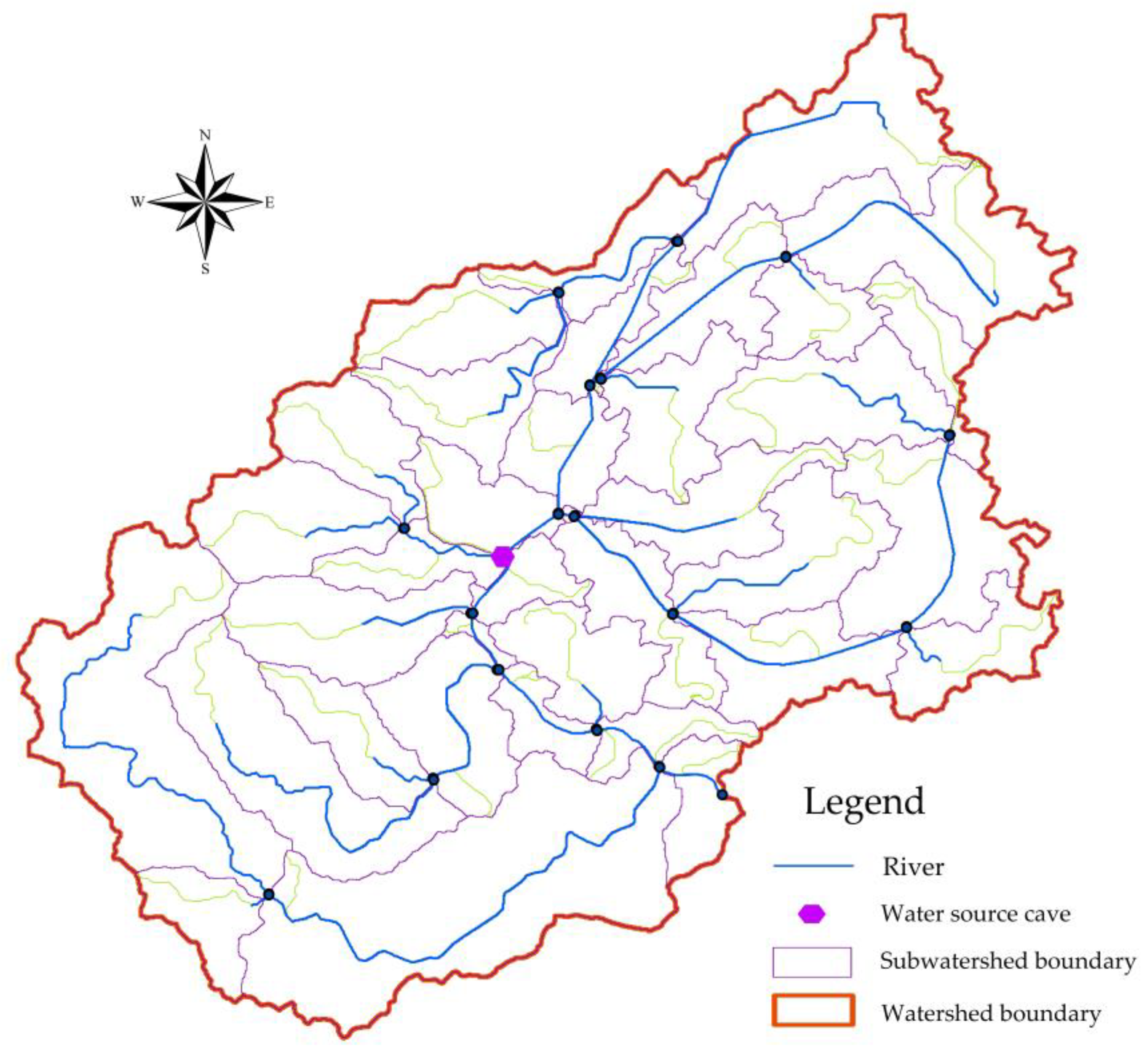
The Xiajia River basin with the main river channel of 35.12 km and a drainage area of 799.20 km², is a typical karst area in Southwest China (Figure 1a). The mainstream in the Xiajia River basin is the Chengbi River (the upper reaches are called the Yangba River), and its main tributaries include the Chaoli, Mengsha, Yaoma, and Dancun River. There is a natural karst cave (water source cave) on the main river channel in southeastern Lingyun County. Most of the water from upstream of the cave belongs to underground undercurrent. The measured precipitation and flow data from 1 January 2002, to 3 September 2018, are recorded by Chaoli station (CLS), Donghe station (DHS), Lingyun station (LYS), and Xiajia station (XJS) (

Table 1. The GPS coordinates and elevation of each station.

Station Code	Station Name	Station Category	Longitude	Latitude	Elevation(m)
20,000,900	Chaoli	Rainfall Station	106°30′14.736″ E	24°14′21.567″ N	625
20,001,300	Donghe	Rainfall Station	106°43′25.983″ E	24°21′37.121″ N	897
20,000,800	Lingyun	Rainfall Station	106°34′26.216″ E	24°20′42.088″ N	444
20,001,000	Xiajia	Hydrological Station	106°38′51.175″ E	24°17′18.718″ N	385

) [44,45,46]. The satellite data used are IMERG early data with a 0.5-h resolution from 12 March 2014, to 3 September 2018, which has the shortest delay. The download space ranges from 24.1° N to 24.6° N, and from 106.3° E to 106.8° E. The spatial grid distribution of the IMERG precipitation data is shown in Figure 1b. Since the coordinated universal time (UTC) of IMERG satellite precipitation data, it is necessary to add an 8-h time difference to convert it into Beijing time to realize the unification of satellite data and ground data time.

2.2. Evaluation Indices

The Correlation coefficient is applied to the accuracy evaluation of IMERG satellite precipitation data at temporal and spatial scales. The Probability of detection, False alarm rate (FAR), and Critical success index (CSI) are selected to evaluate the precipitation detection capability. The indexes mentioned above are calculated by the following equation [47]:

$$R=\frac{{\displaystyle \sum _{i=1}^N(x_i-\overline{X})}(x_{0i}-\overline{X_0})}{\sqrt{{\displaystyle \sum _{i=1}^N(x_i-\overline{X}}}{)}^2\sqrt{{\displaystyle \sum _{i=1}^N(x_{0i}-\overline{X_0}}{)}^2}}$$

(1)

$$\mathrm{POD}=\frac{H}{H+M}$$

(2)

$$\mathrm{FAR}=\frac{F}{H+F}$$

(3)

$$\mathrm{CSI}=\frac{H}{H+F+M}$$

(4)

where $N$ is the number of samples; $x_i$ is the precipitation observed by the ground stations, mm; $x_{0i}$ is the precipitation observed by IMERG, mm; $\overline{X}$ is the average precipitation observed by the ground stations, mm; $\overline{X_0}$ is the average precipitation observed by IMERG, mm; $H$ is the precipitation observed by the ground station and IMERG, simultaneously; $M$ is the precipitation observed by the ground stations but fail to be observed by IMERG; $F$ is the precipitation observed by IMERG but fail to be observed by the ground stations.

The Nash efficiency coefficient (NSE) and the RMS standard deviation ratio (RSR) was selected to evaluate the performance of the SWAT model, and the evaluation criteria [48,49] was shown in

Table 2. The evaluation criteria for RSR and NSE.

Evaluation Level	RSR	NSE
Very good	0.00 ≤ RSR ≤ 0.50	0.75< NSE ≤ 1.00
Good	0.50 < RSR ≤ 0.60	0.65< NSE ≤ 0.75
Satisfactory	0.60 < RSR≤ 0.70	0.50< NSE ≤ 0.65
Unsatisfactory	RSR> 0.70	NSE≤ 0.50

.

$$\mathrm{NSE}=1-\frac{{\displaystyle \sum _{i=1}^n{(q_i^{obs}-q_i^{sim})}^2}}{{\displaystyle \sum _{i=1}^n{(q_i^{obs}-{\overline{q}}^{obs})}^2}}$$

(5)

$$\mathrm{RSR}=\sqrt{\frac{{\displaystyle \sum _{i=1}^n{(q_i^{obs}-q_i^{sim})}^2}}{{\displaystyle \sum _{i=1}^n{(q_i^{obs}-{\overline{q}}^{obs})}^2}}}$$

(6)

where $i$ is the series number, $q^{obs}$ is the measured flow, ${\overline{q}}^{obs}$ is the mean value of the measured flow, $q^{sim}$ is the simulated flow, ${\overline{q}}^{sim}$ is the mean value of the simulated flow, and $n$ is the total number of observations.

2.3. Data Correction Method

The fusion correction methods such as the Linear regression method, the Mean deviation correction method, the Bayesian fusion method, the Geographic weighted regression method, and the Geographic difference analysis (GDA) method, can be adopted to improve the accuracy of the satellite data [50,51]. In this study, the GDA method was applied due to its advantages of good correction effect and simple calculation. The specific correction steps of the GDA method are as follows [52]:

(1) Firstly, calculate the difference between the precipitation measurement for each ground station and the corresponding satellite pixel;

(2) Then, the Inverse distance weighted interpolation (IDW) method is applied to analyze the spatial interpolation of the rainfall differences to obtain a difference map;

(3) Finally, calibrate (correct) the satellite rainfall estimates with the difference map.

2.4. SWAT Model

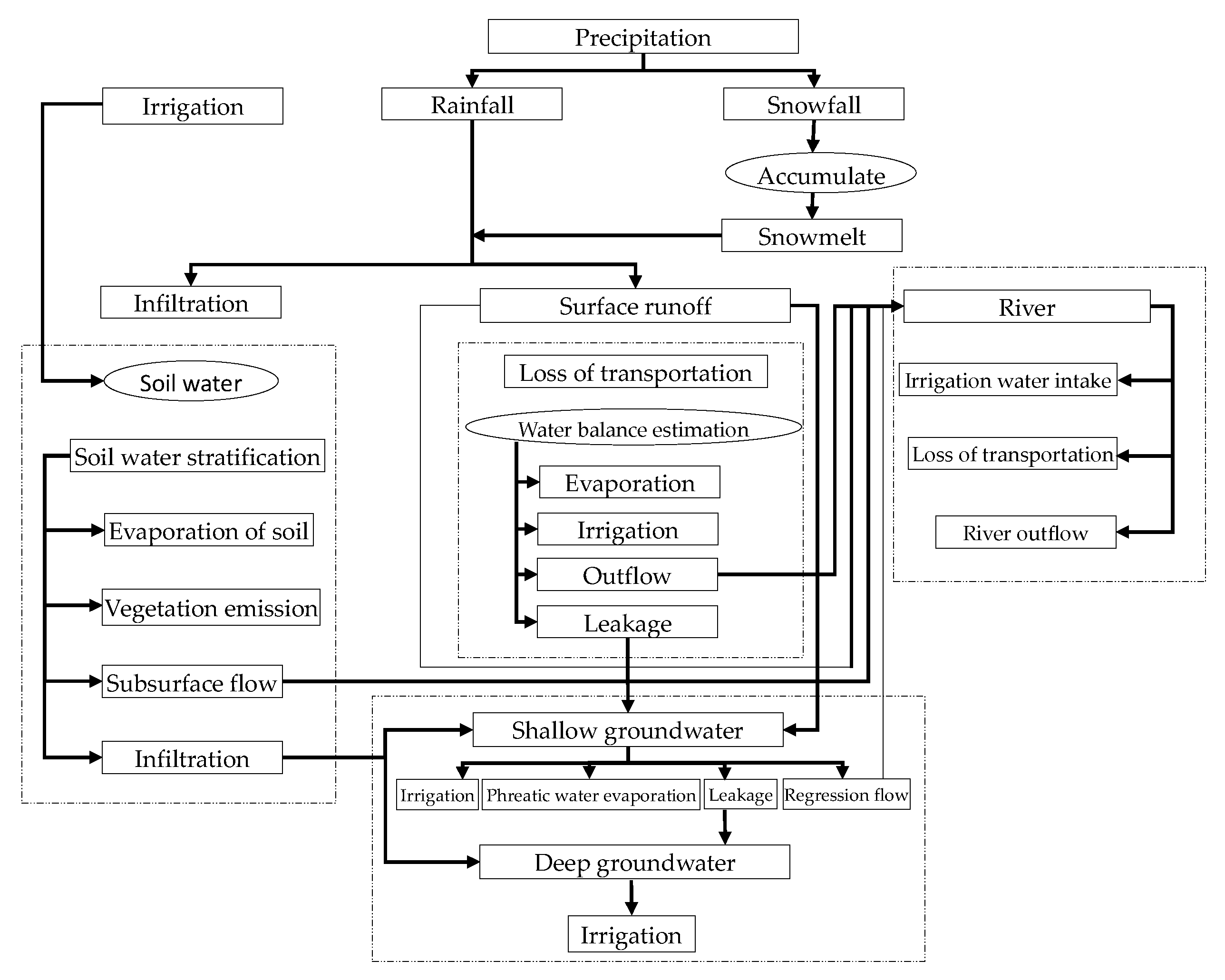
The Soil and Water Assessment Tool (SWAT) model was a distributed hydrological model and suitable for multiple time scale runoff simulations. The model, developed by USDA-ARS, includes eight modules called weather, hydrology, nutrients, sediment, land cover, management measures, river course process, and water body. The runoff, sediment, nutrients, and other processes can be simulated by inputting the terrain, land cover, soil type, weather, pollution source, and other information. The SWAT model has been widely used in runoff simulation, sediment transport simulation, and non-point source pollution prediction since the advantages of easy access to parameters, high calculation efficiency, and continuous simulation [6,53,54]. A schematic diagram of the SWAT model is shown in Figure A1 of Appendix A.

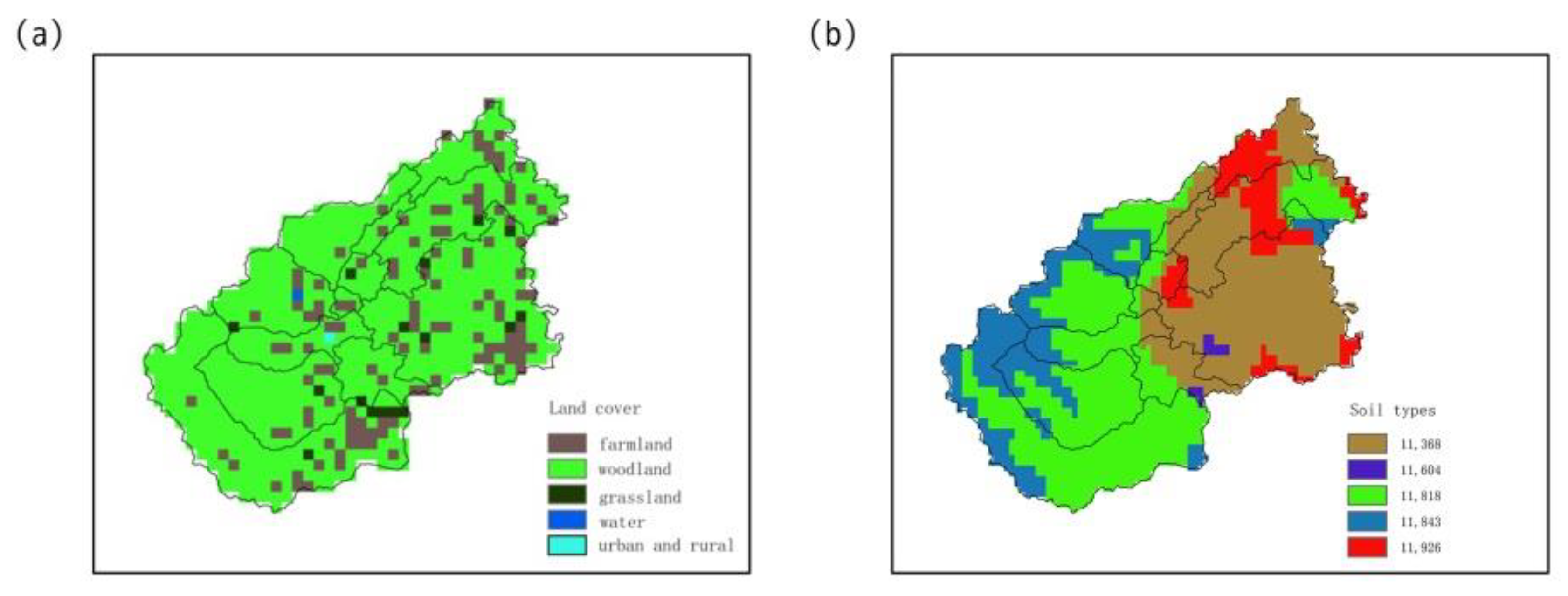
In this study, the original DEM is processed by using the Stream burning method [55], and the cumulative threshold of confluence is set to 1000 by using the watershed extraction tool of ArcSWAT(United States Department of Agriculture, Washington, USA) software (ArcSWAT is an ArcGIS-ArcView extension and interface for SWAT) to obtain the extracted Xiajia River basin (Figure 2). The land cover data of the study area are from the IGBP_LUCC (Food and Agriculture Organization of the United Nations, Rome, Italy) (International Geosphere-Biosphere Programme_Land Use/Cover Change) database and are reclassified according to the type and number specified by the SWAT model. The spatial distribution of land cover is shown in Figure 3a. Besides, the soil data of the study area are from the HWSD(Food and Agriculture Organization of the United Nations, Rome, Italy) (Harmonized World Soil Database) database, some parameters are directly copied from HWSD, the others are recalculated by SPAW (Washington State University, Washington, USA) (Soil-Plant-Air-Water) software, and the spatial distribution of soil data is shown in Figure 3b. According to the weight of 5% of land cover, 20% of soil data, and 20% of slope, 114 hydrological response units (HRU) are generated.

Considering the series of satellite data is relatively short (2014–2018), the static parameter method is applied to calibrate and validate the model parameters based on the ground data. In more detail, set January 2002 to February 2014 as the calibration period, and March 2014 to September 2018 as the validation period.

The weather data needed for the SWAT model include precipitation, relative humidity, solar radiation, temperature, and wind speed. The precipitation data used in this study are measured by the ground stations and IMERG early. The other weather data are calculated depend on the CMADS-V1.1 dataset (spatial resolution is 0.25 × 0.25) and the weather generator. Then, the generated weather data are transformed into SWAT format and imported into the SWAT model. Considering the flow characteristics of the karst area in the Xiajia River basin, the SWAT model is adjusted by adding a reservoir unit to the river channel where the water source cave is located and 7 model parameters named RES_K, RES_RR, RES_ESA, RES_PSA, RES_EVOL, RES_PVOL, and RES_VOL, are added. As a result, a total of 17 parameters called CN2, ALPHA_BF, GW_DELAY, GWQMN, ALPHA_BNK, CH_K2, GW_REVAP, REVAPMN, ESCO, CH_N2, RES_K, RES_RR, RES_ESA, RES_PSA, RES_EVOL, RES_PVOL, and RES_VOL are calibrated by using SWAT-CUP software. The physical meaning and the calibration results of the parameters are shown in

Table A1. Daily calibration results of SWAT model parameters.

Serial Number	Parameter	Meaning	Initial Value	Unit	Final Value
1	CN2	SCS Curve number (AMC II)	60~92	/	69.76~100
2	ALPHA_BF	Base flow recession constant	0.048	day	0.31
3	GW_DELAY	Groundwater time delay	31	day	8.25
4	GWQMN	Regression water level threshold	1000	mm	1360.54
5	ALPHA_BNK	Baseflow factor	0	/	0.31
6	CH_K2	The permeability coefficient of the main channel	0	mm/hour	344.99
7	GW_REVAP	Reavp coefficient of groundwater	0.02	/	0.16
8	REVAPMN	Occurrence reavp water level threshold	750	mm	1106.43
9	ESCO	Soil evaporation compensation factor	0.95	/	0.62
10	CH_N2	Manning coefficient of main channel	0.014	/	0.14
11	RES_K	Permeability coefficient of reservoir	5	mm/hour	7.09
12	RES_RR	Average daily discharge	100	m3/s	175.08
13	RES_ESA	Area of non overflow reservoir	3177.1	ha	8461.61
14	RES_PSA	Area of normal overflow reservoir	2051.9	ha	8294.77
15	RES_EVOL	Extraordinary flood storage capacity	90,000,000	104 m3	48,893,760.00
16	RES_PVOL	Normal flood storage capacity	100,000	104 m3	61,111.90
17	RES_VOL	Initial storage capacity	5000	104 m3	11,924.99

and

Table A2. Monthly calibration results of SWAT model parameters.

Serial Number	Parameter	Meaning	Initial Value	Unit	Final Value
1	CN2	SCS Curve number (AMC II)	60~92	/	60.56~92.86
2	ALPHA_BF	Base flow recession constant	0.048	day	0.34
3	GW_DELAY	Groundwater time delay	31	day	−124.41
4	GWQMN	Regression water level threshold	1000	mm	2636.32
5	ALPHA_BNK	Base flow factor	0	/	0.11
6	CH_K2	Permeability coefficient of main channel	0	mm/hour	159.31
7	GW_REVAP	Reavp coefficient of groundwater	0.02	/	0.15
8	REVAPMN	Occurrence reavp water level threshold	750	mm	1489.71
9	ESCO	Soil evaporation compensation factor	0.95	/	0.91
10	CH_N2	Manning coefficient of main channel	0.014	/	0.04
11	RES_K	Permeability coefficient of reservoir	5	mm/hour	0.45
12	RES_RR	Average daily discharge	100	m3/s	30.00
13	RES_ESA	Area of non-overflow reservoir	3177.1	ha	13,085.54
14	RES_PSA	Area of normal overflow reservoir	2051.9	ha	1501.43
15	RES_EVOL	Extraordinary flood storage capacity	90,000,000	104 m3	45,000,000.00
16	RES_PVOL	Normal flood storage capacity	100,000	104 m3	285,142.00
17	RES_VOL	Initial storage capacity	5000	104 m3	5233.83

of Appendix A.

3. Results and Discussion

3.1. Accuracy Analysis of IMERG Satellite Precipitation Data

3.1.1. Temporal Scale Accuracy Evaluation

The R index was applied to evaluate the accuracy of IMERG early precipitation data at the temporal scale; in other words, to show how well the IMERG satellite precipitation data matches the precipitation data observed by ground stations at the temporal scale—the results are shown in Figure 4. As can be seen from Figure 4, the R index value between the IMERG satellite precipitation data and the precipitation data observed by ground stations at 1-h, 3-h, daily and monthly time scales are 0.412, 0.492, 0.667 and 0.884, respectively, indicating that the R value increases with increasing time scale. That is, the larger the time scale, the greater the rainfall accuracy of IMERG satellite precipitation data. Additionally, the degree of dispersion of rainfall data also increases with increasing time scales. At the 1-h scale (Figure 4a), the IMERG early data are most discrete, which significantly underestimates (negative bias) the ground data. At the monthly scale, the IMERG early data are least discrete, which underestimates the ground data to a certain extent (negative bias). The lower limit values of significant tests for R in different time scales are list in

Table 3. The lower limit value of a significant test for R at different time scales.

Time Scale	Sample Size	$\mathit{\alpha }=0.05$	$\mathit{\alpha }=0.01$
1 h	39,288	0.009888	0.012995
3 h	13,096	0.017127	0.022508
daily	1638	0.049436	0.063629
monthly	54	0.268086	0.347652

[56]. The lower limit values range from 0.009888 (1-h scale) to 0.268086 (monthly scale) at a confidence level $\alpha =0.05$ and range from 0.012995 (1-h scale) to 0.347652 (monthly scale) at a confidence level $\alpha =0.01$.

3.1.2. Spatial Scale Accuracy Evaluation

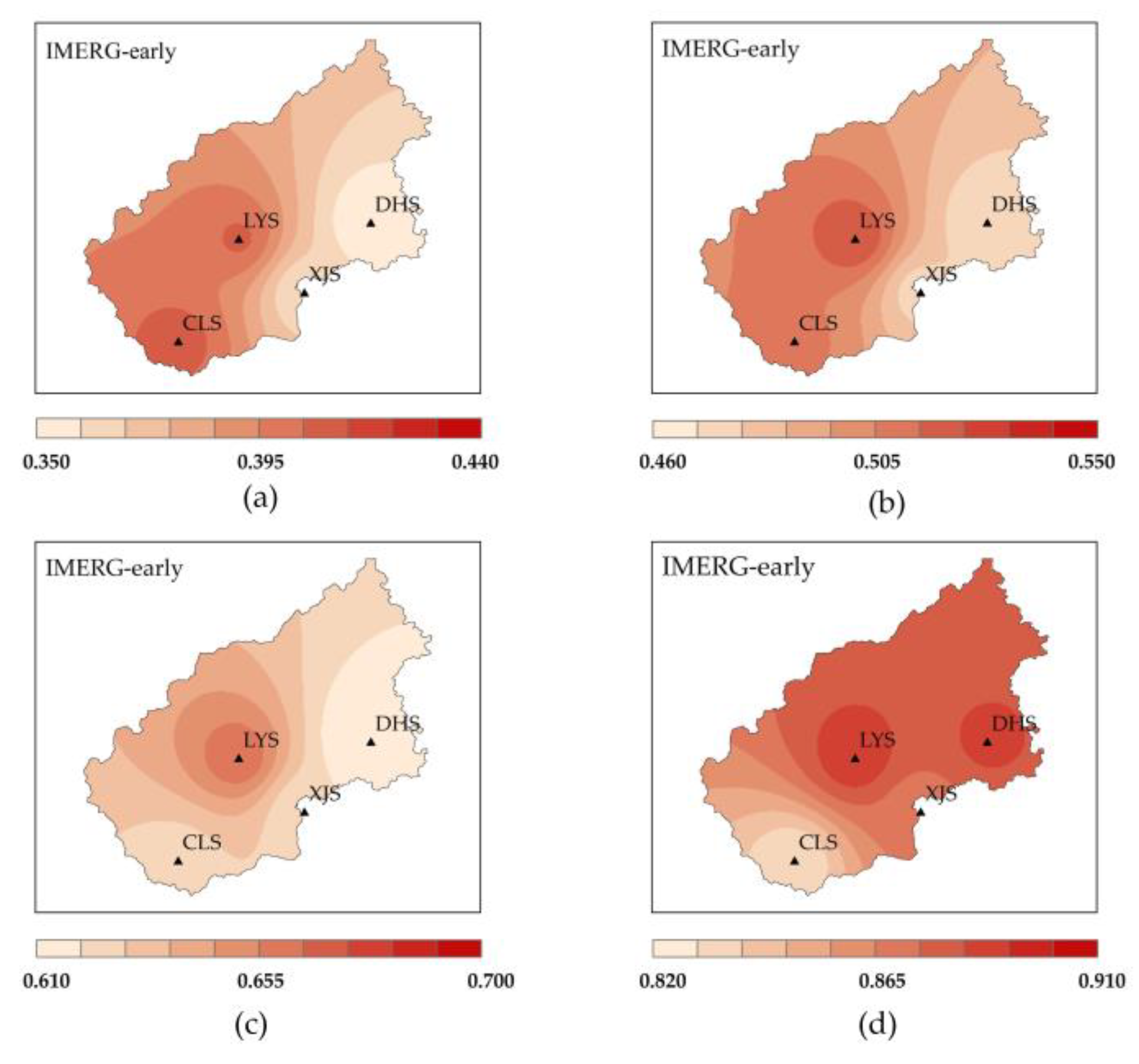
Firstly, the R values of the IMERG early precipitation data (corresponding to each station) were calculated, and then the IDW method was used to analyze the spatial distribution of the R values to evaluate the accuracy of IMERG precipitation data at spatial scale, and the results are shown in Figure 5. For the 1 h scale, the R values range from 0.350 to 0.440, and the values in the central and western regions of the basin are larger than those in the other parts, indicating a higher accuracy of the IMERG precipitation data in the central and western parts of the basin. For the 3 h scale, the R values range from 0.460 to 0.550, and the values in the central and western regions of the basin are larger than those in the other parts, indicating a higher accuracy of the IMERG precipitation data in the central and western parts of the basin. For daily scale, the R values range from 0.610 to 0.700, and the values in the central regions of the basin are larger than those in the other parts, indicating a higher accuracy of the IMERG precipitation data in the central parts of the basin. For a monthly scale, the R values range from 0.820 to 0.910, and the values in the central and eastern regions of the basin are larger than those in the other parts, indicating a higher accuracy of the IMERG precipitation data in the central and eastern parts of the basin. Overall, the R values show an increasing pattern with an increasing time scale.

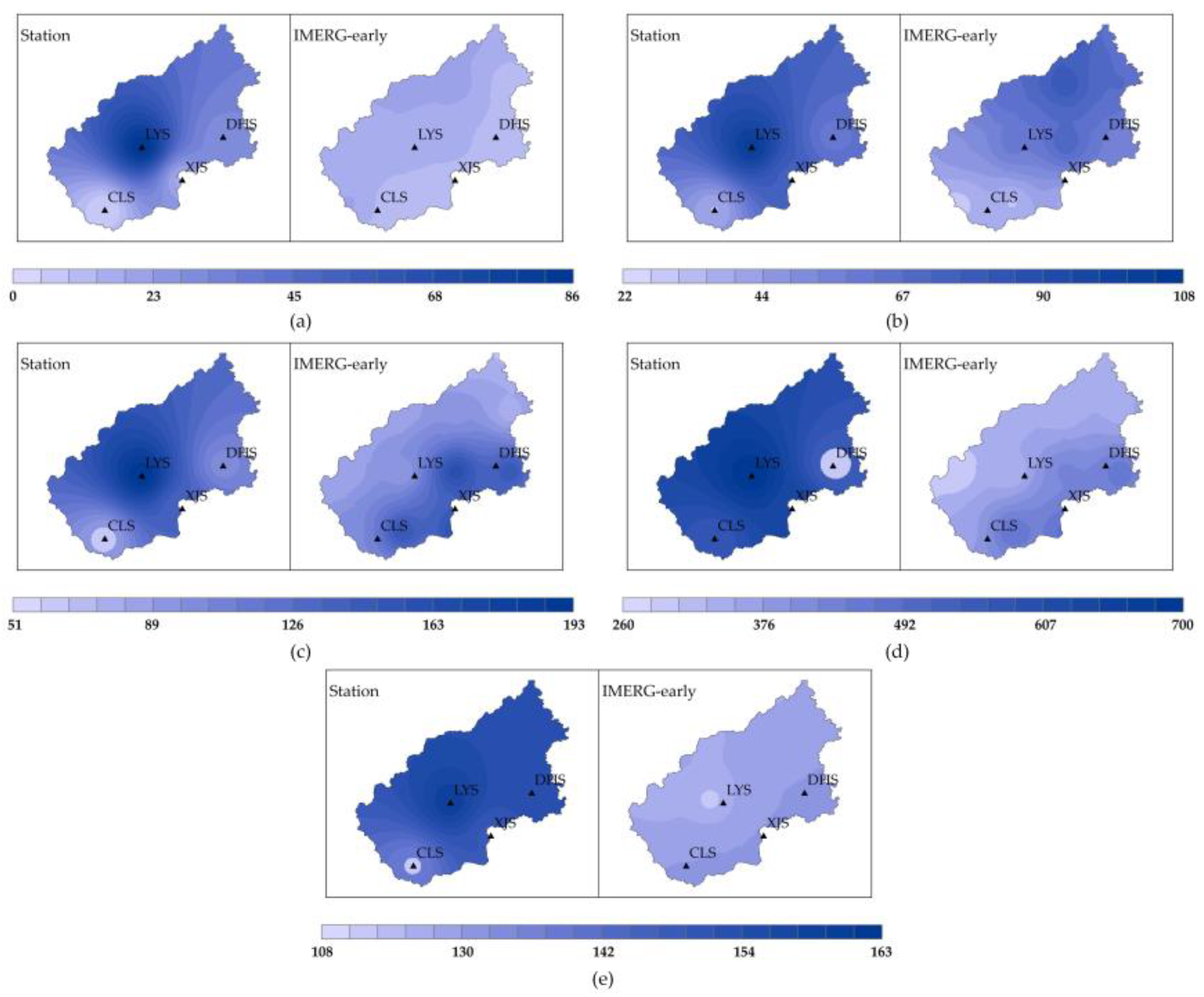
Furthermore, the maximum 1-h precipitation, maximum 3-h precipitation, maximum 1-day precipitation, maximum 1-month precipitation, and the average monthly rainfall from 2014–2018 were selected to evaluate the spatial accuracy of rainfall extremes and average monthly rainfall, and the results are shown in Figure 6. Overall, the IMERG early data at all time scales significantly underestimate the extreme precipitation and average monthly precipitation compared with that of the ground stations. Taking the maximum 1-h precipitation as an example, the values observed by ground stations are larger than those observed by IMERG early, and the values observed by ground stations show a characteristic that the value of the maximum 1-h precipitation is larger in the middle part of the basin while the value observed by IMERG early fails to reflect this characteristic.

3.1.3. Detection Capability Evaluation

The Probability of detection (POD), False alarm rate (FAR), and Critical success index (CSI) were applied to evaluate the precipitation detection capability of IMERG data, and the results are summarized in

Table 4. The precipitation detection capability of IMERG data. Unit: %.

Parameter	1 H	3 H	Daily	Monthly
POD	47.33	54.81	71.57	100.00
FAR	50.99	40.34	19.43	0.00
CSI	31.71	39.99	61.04	100.00

. The POD values range from 47.33% to 100% and show a tendency to increase with increasing time scale. The FAR values range from 0.00% to 50.99% and show a tendency to decrease with increasing time scale. The CSI values range from 39.99% to 100% and show a tendency to increase with increasing time scale. In summary, the precipitation detection capability of the IMERG early gradually increases as the time scale increases.

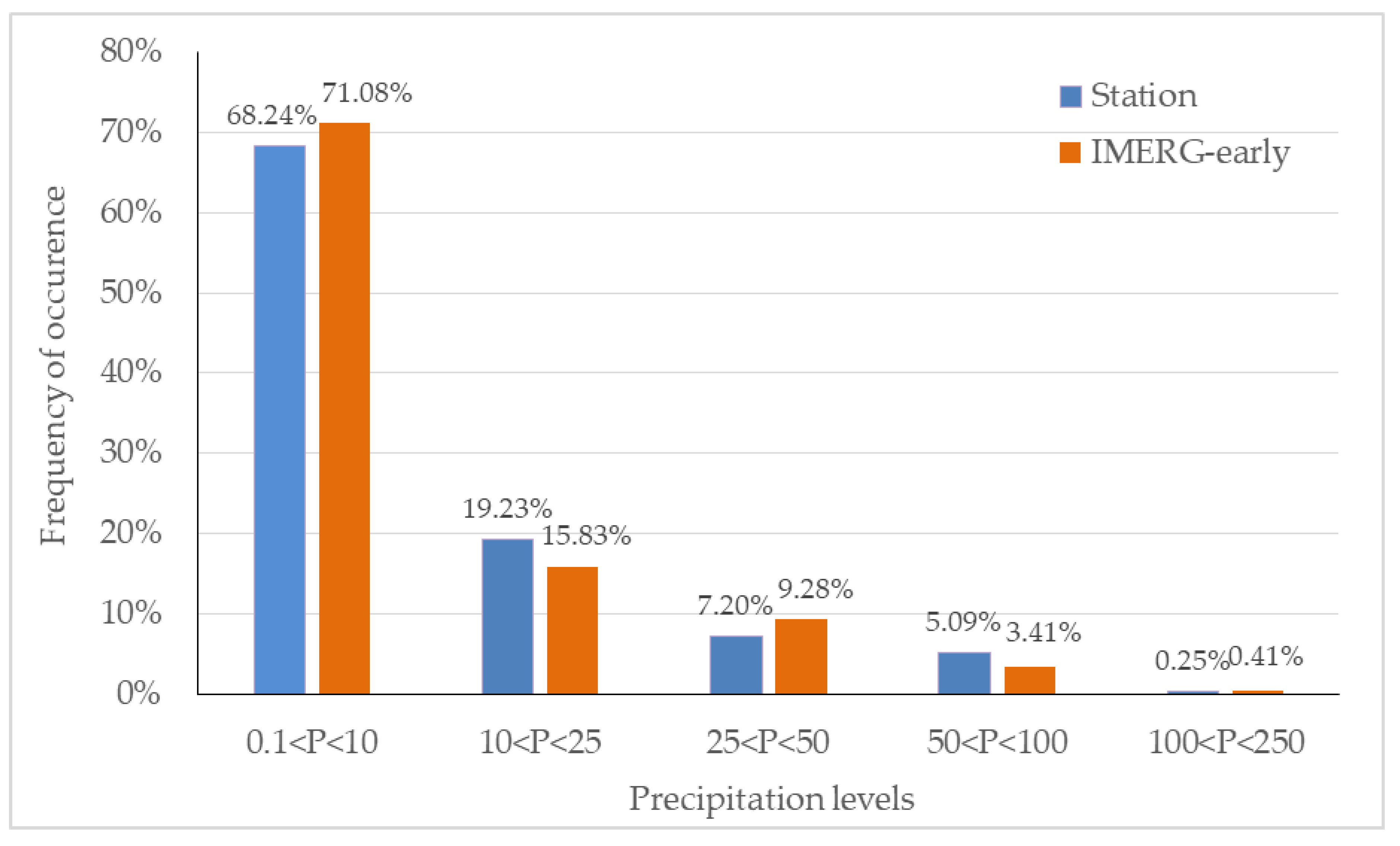
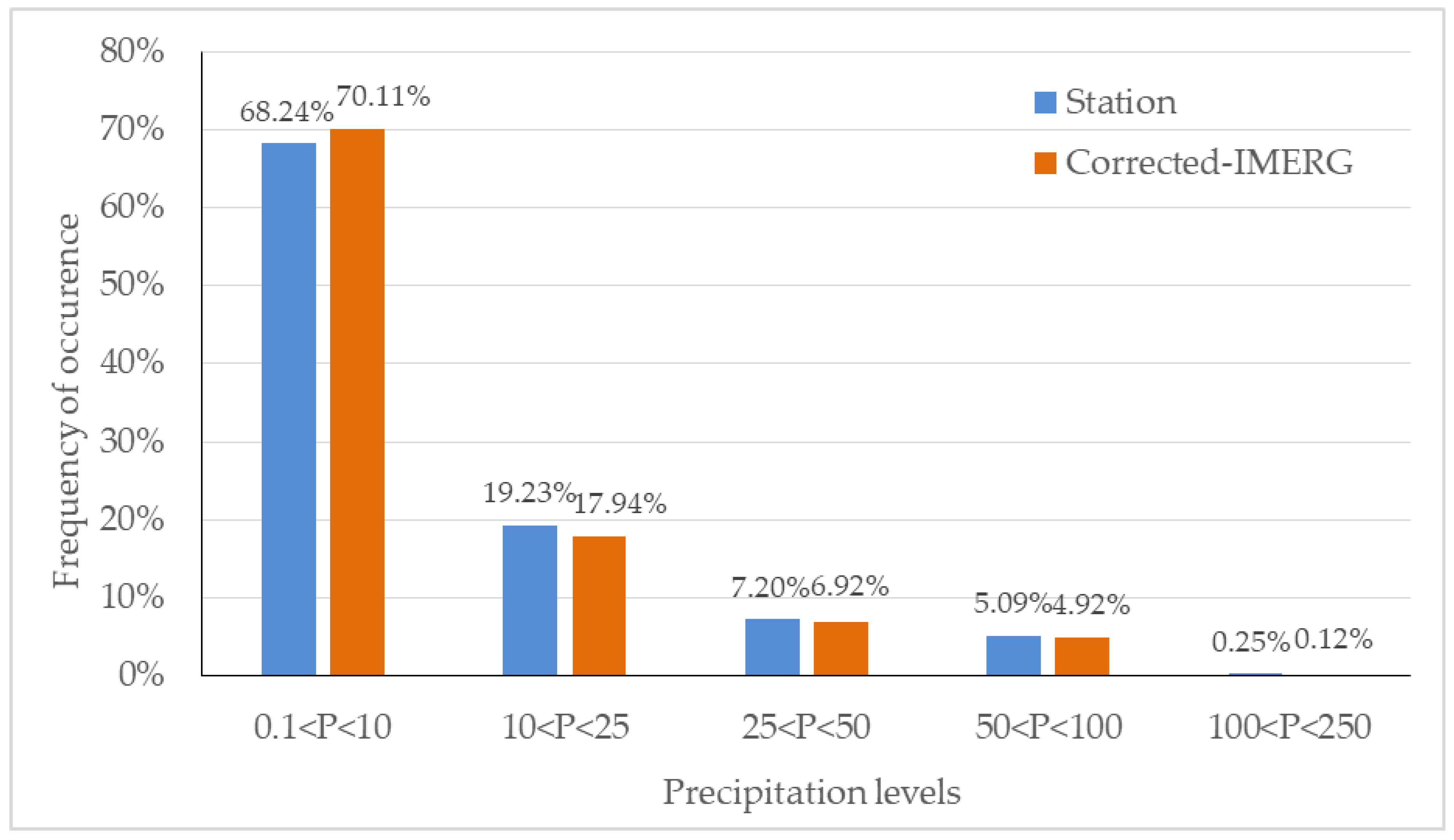
Besides, this study further analyzed the ability of IMERG early to identify the frequency of occurrence of various rainfall levels for the period from March 2014 to September 2018. As suggested by the Chinese national industry standard, GB/T 28592-2012 precipitation classification [57], the rainfall level are determined as 24 h precipitation is light rain at 0.1–9.9 mm, moderate rain at 10.0–24.9 mm, heavy rain at 25.0–49.9 mm, rainstorm at 50.0–99.9 mm, heavy rainstorm at 100.0–249.9 mm and extraordinary rainstorm at 250.0 mm or above. As shown in Figure 7, as the rainfall level increases (from light rain to extraordinary rainstorm), the less frequent the rainfall occurs. Besides, compared to station rainfall, satellite rainfall overestimates the frequency of light rainfall, heavy rain, and extraordinary rainstorm while underestimating the frequency of moderate rain and rainstorm.

3.2. Runoff Simulation Results—Using the IMERG Early Data

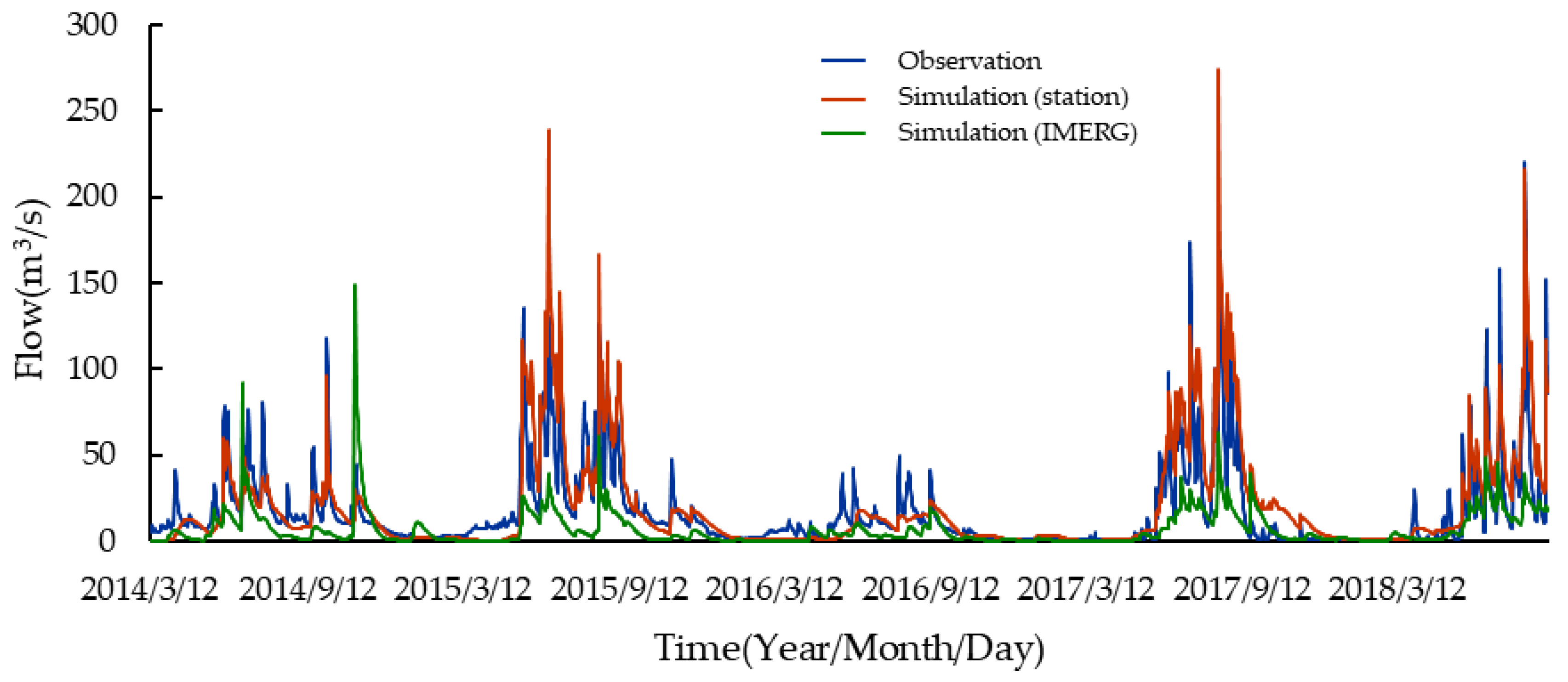
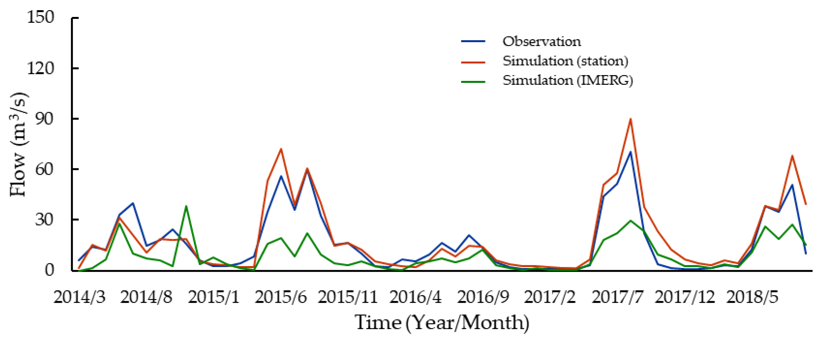
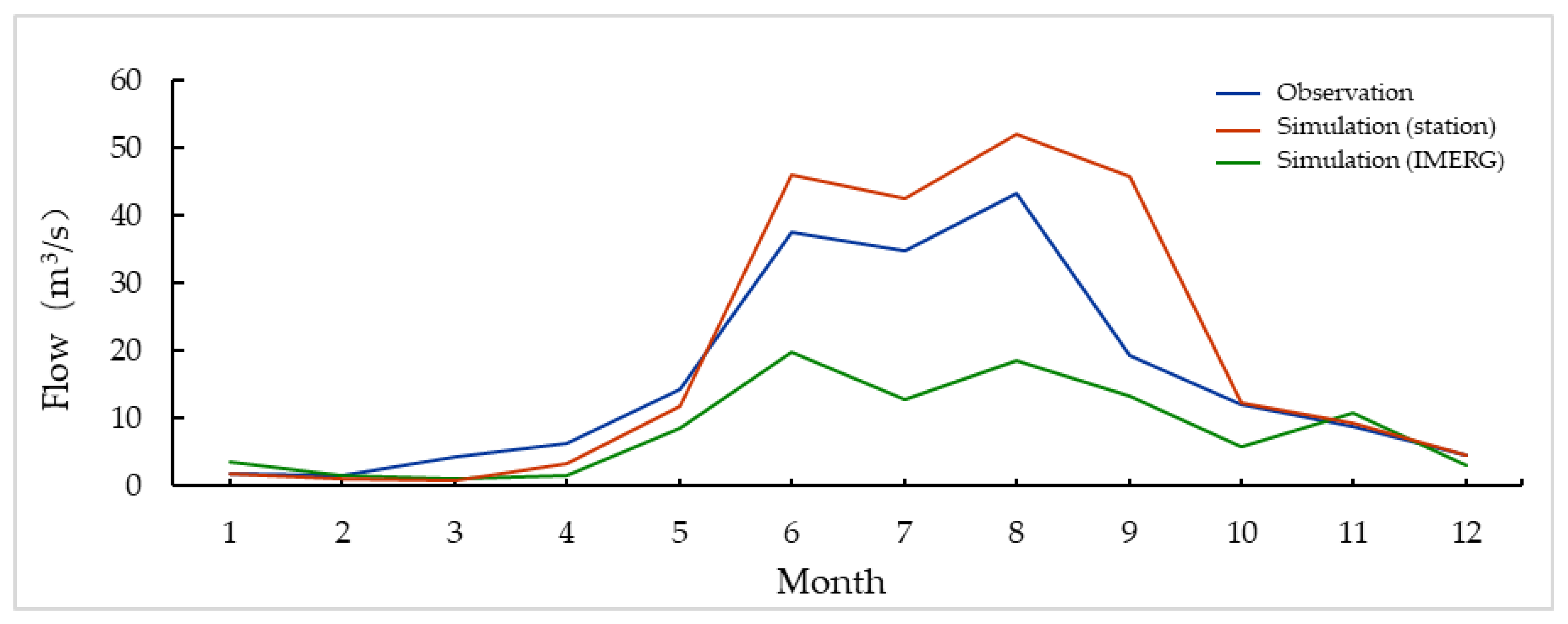
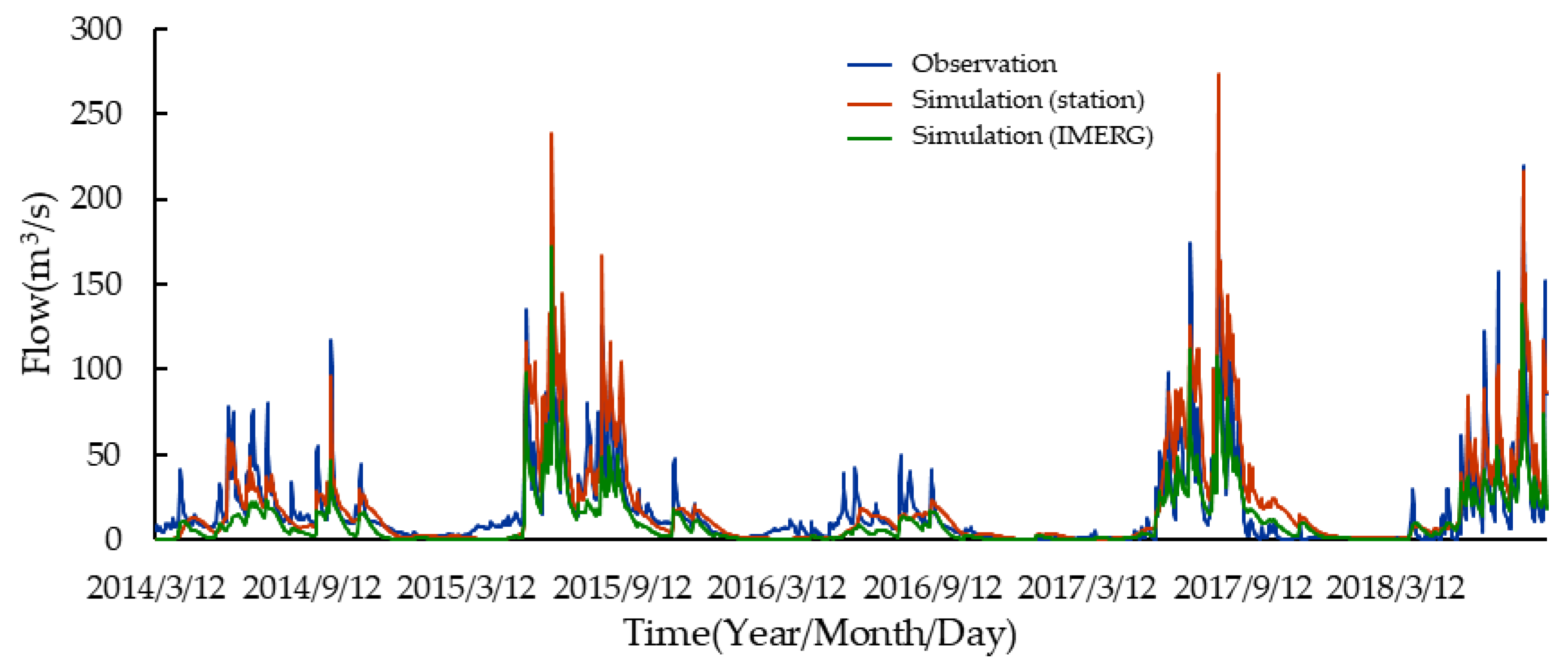
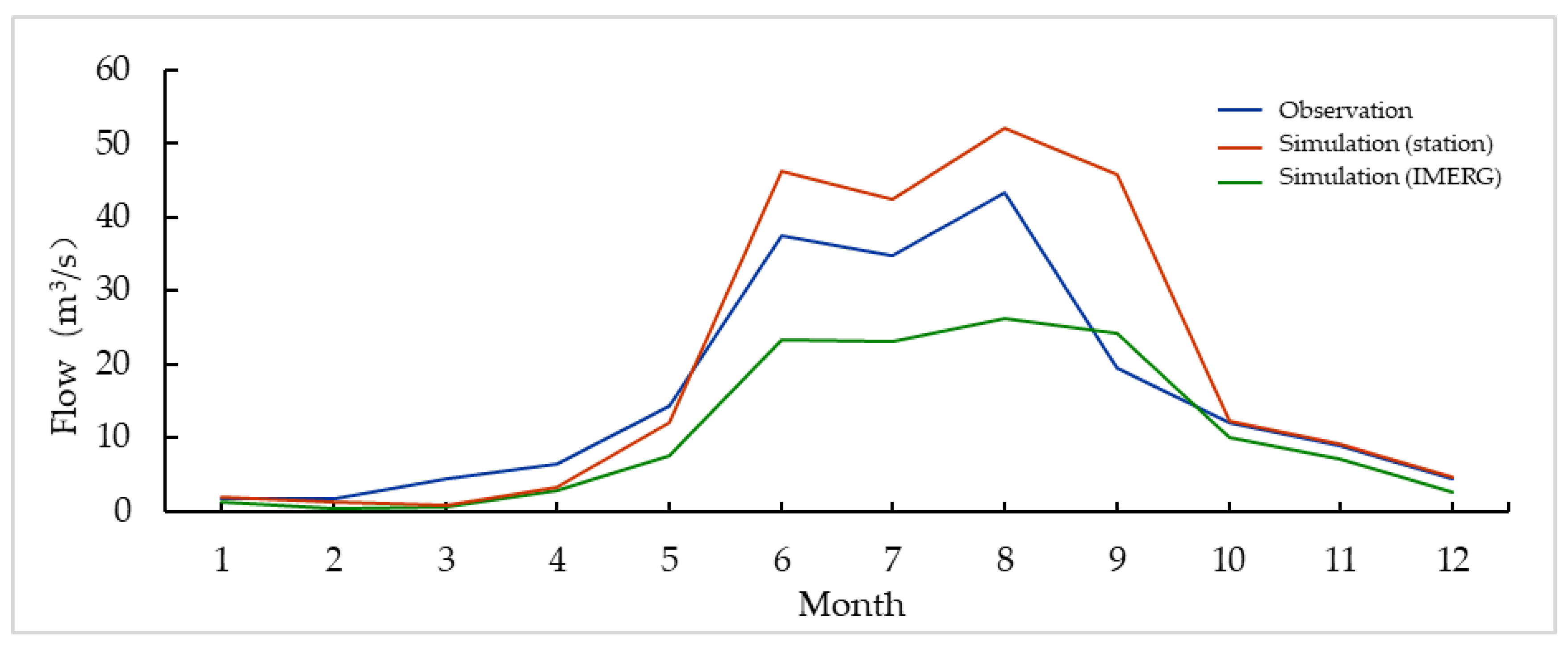
After being calibrated by using the precipitation observed by the ground station, the SWAT model was driven by the IMERG early data to obtain the runoff process on the daily, monthly and multi-year monthly mean scales in the validation period to evaluate the application of the IMERG early data in long-term runoff simulation, and the results are shown in Figure 8, Figure 9 and Figure 10 and

Table 5. The NSE and RSR results.

Scales	Station		IMERG
	NSE	RSR	NSE	RSR
daily	0.60	0.63	0.17	0.92
monthly	0.78	0.46	0.32	0.81
multi-year monthly mean	0.64	0.60	0.49	0.71

. The simulated daily runoff reflected the periodic change in the measured flow, but there were differences in the value and the wet and dry trend. For example, 2014 should be a normal year according to the measured values, while the simulations show 2014 as a wet year. Besides, 2015, 2017, and 2018 should be wet years, but the simulated flows in these years are relatively small (Figure 8). For the simulated monthly and mean–year monthly runoff process (Figure 9 and Figure 10), the overall runoff process was underestimated, especially, the high value was wrongly simulated at the end of 2014 for the monthly runoff process. Furthermore, the NSE and RSR results are shown in Table 5. The NSE and RSR for the daily runoff simulation are 0.17 and 0.92, and the values are 0.32 and 0.81 for the monthly runoff simulation, and 0.49 and 0.71 for the simulation of the monthly results for the mean year. The above results indicate that the runoff simulation results of IMERG data in the validation period are poor, and the simulation results need to be improved, implying that the IMERG data cannot be used without any correction.

3.3. Accuracy Analysis of Corrected IMERG Satellite Precipitation Data

Temporal Scale Accuracy Evaluation for Corrected IMERG

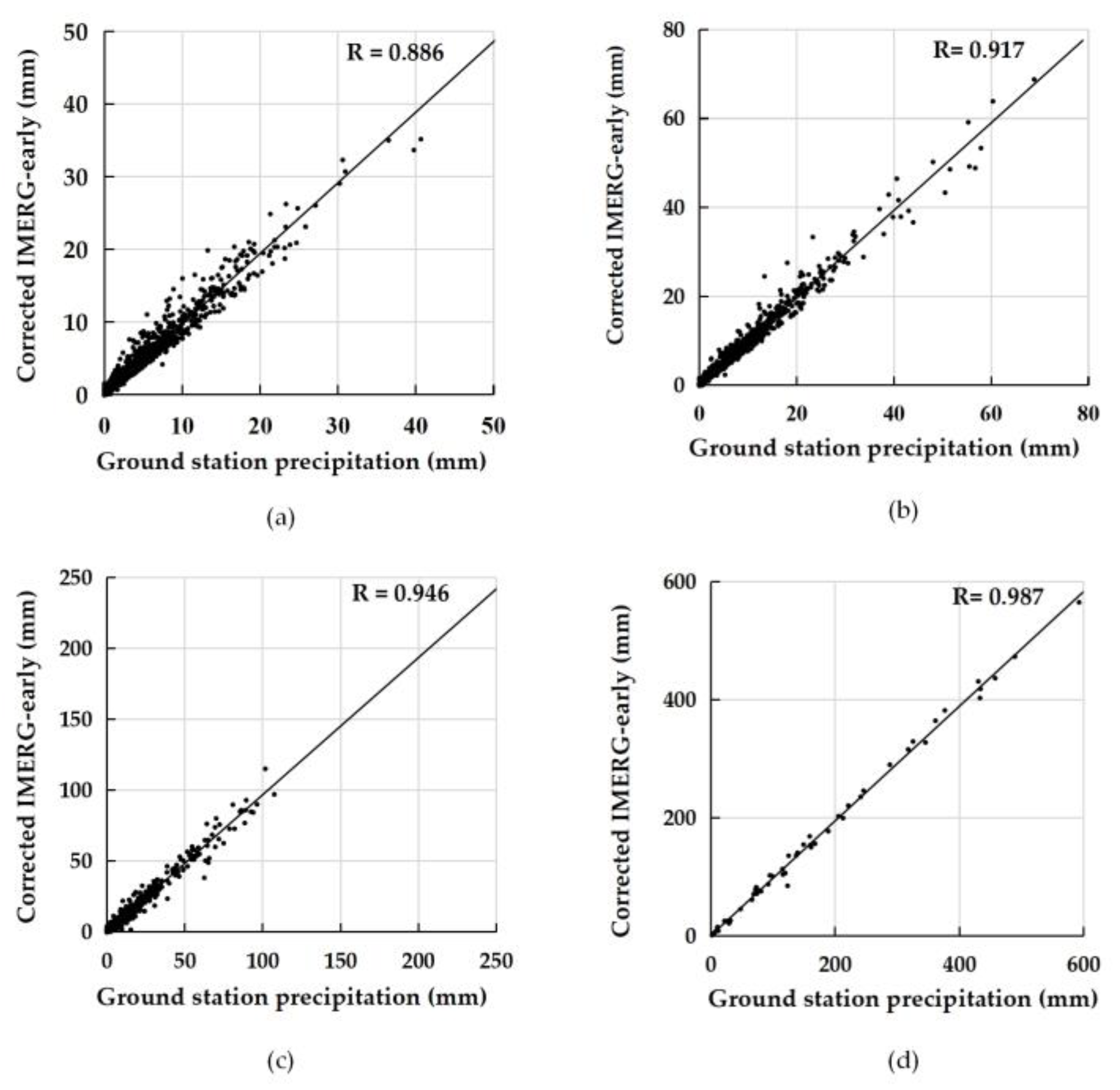
The R index was applied to evaluate the accuracy of corrected IMERG early precipitation data at the temporal scale, in other words, to show how well the corrected IMERG satellite precipitation data matches the precipitation data observed by ground stations at the temporal scale, and the results are shown in Figure 11. As can be seen from Figure 11, the R index value between the corrected IMERG satellite precipitation data and the precipitation data observed by ground stations at 1-h, 3-h, daily and monthly time scales are 0.886, 0.917, 0.946 and 0.987, respectively, showing that the R value increases with increasing time scale. That is, the larger the time scale, the greater the rainfall accuracy of corrected IMERG satellite precipitation data. Additionally, a comparison with the R values in Figure 4 shows that the R values between the corrected IMERG satellite precipitation data and the precipitation data observed by ground stations have improved significantly, with improvement values ranging from 0.103 to 0.474. It can also be seen from Figure 11 that the correlation of the corrected IMERG early data is close at the scale of 1-h, 3-h, day, and month, they are all distributed near the 45° line, and there is no obvious positive or negative deviation.

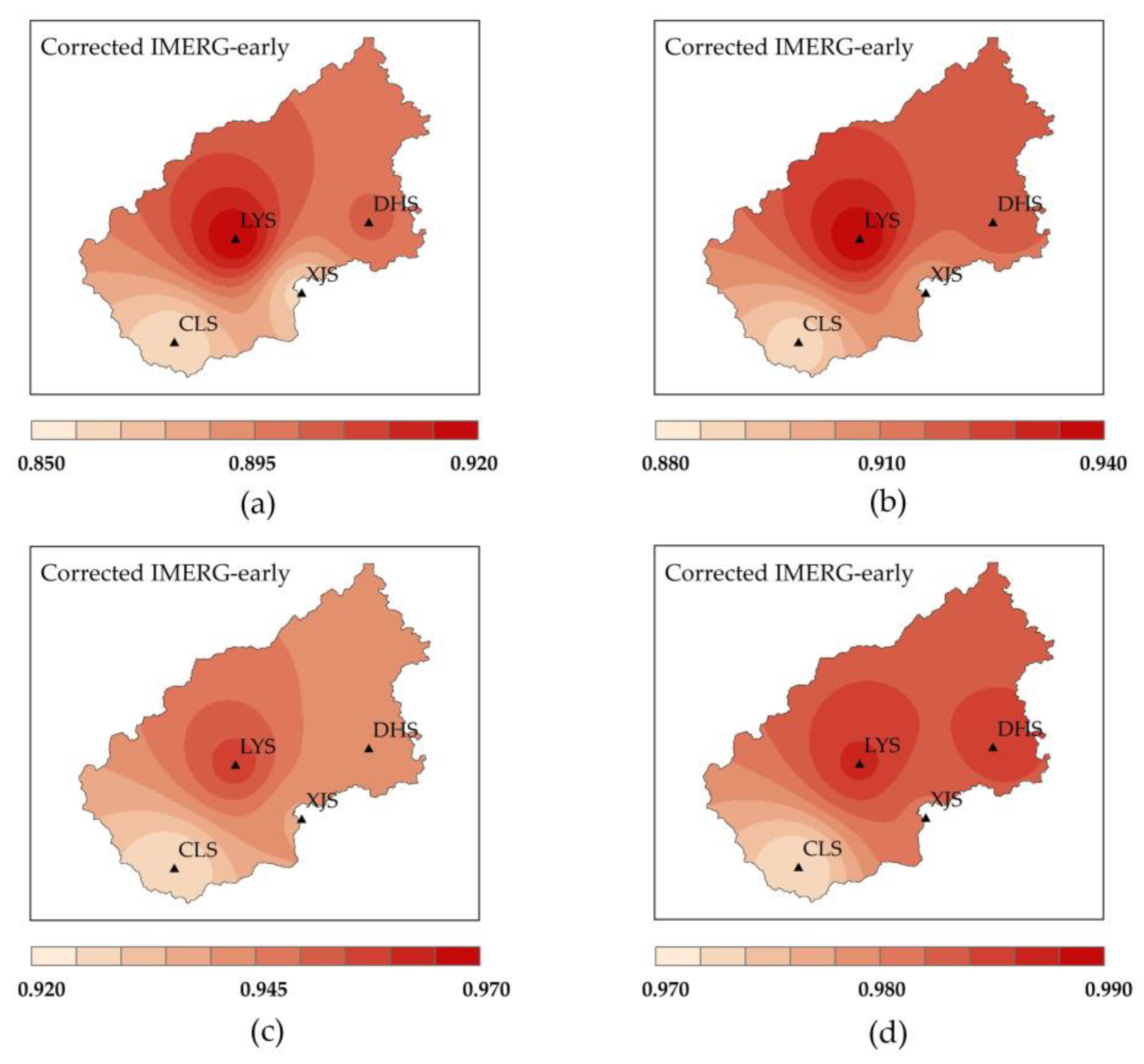
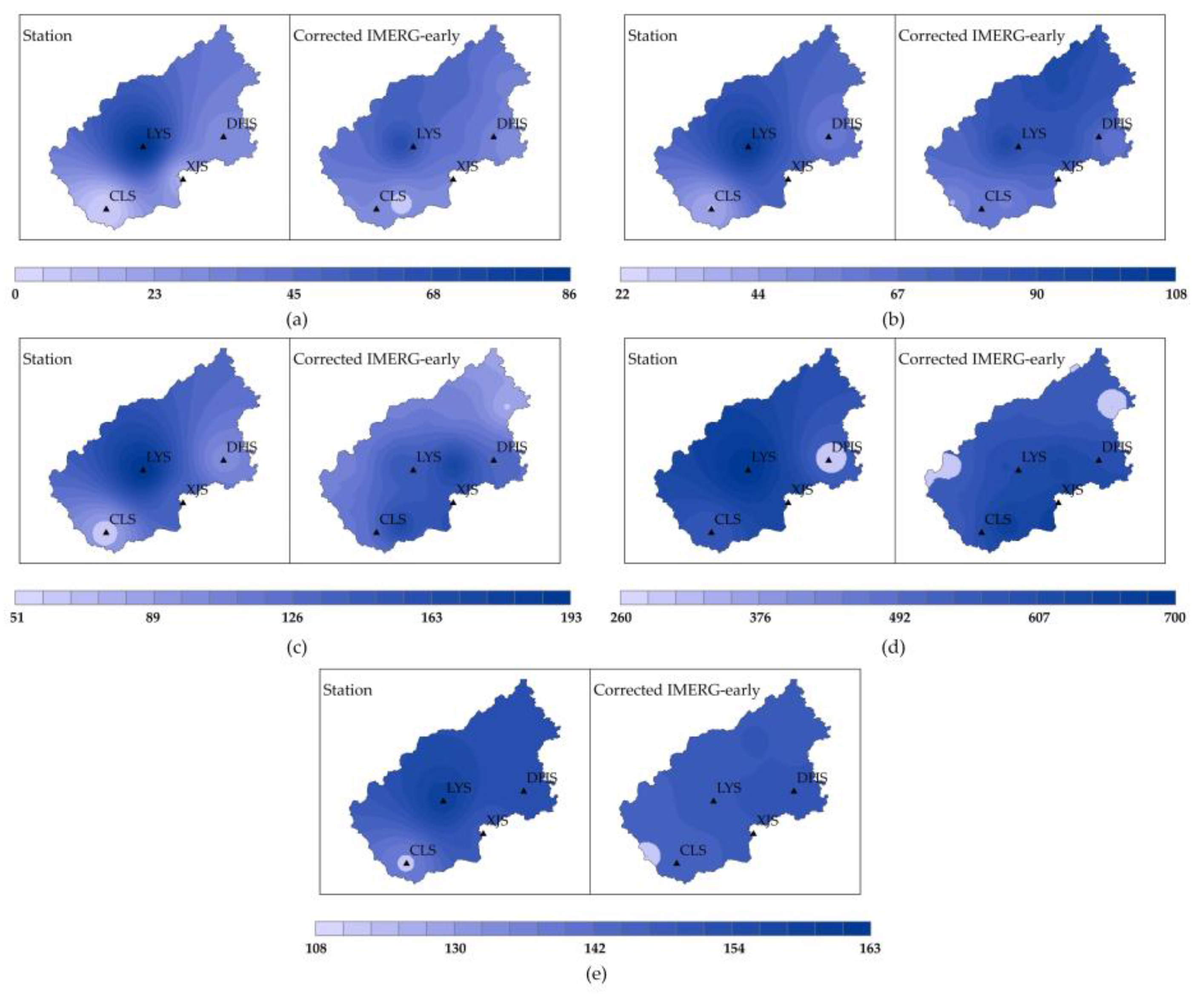
The R spatial distribution for the corrected IMERG precipitation data at various time scales is shown in Figure 12. The spatial analysis of the R of the corrected IMERG data shows that the correlations between the corrected IMERG data and the precipitation observed by the ground station are better than that of the original IMERG early data in most parts of the basin, and the R values are higher in the middle of the basin at all time scales. For 1-h scale, the R values range from 0.850 to 0.920, and the value is 0.880–0.940 for 3-h scale, 0.920–0.970 for daily scale, and 0.970–0.990 for a monthly scale. Overall, the R values showed an increasing pattern with an increasing time scale. Furthermore, the IDW method is used for the spatial interpolation of the maximum 1-h precipitation, maximum 3-h precipitation, maximum 1-day precipitation, maximum 1-month precipitation and average monthly precipitation data in the study area from March 2014 to September 2018, and the spatial distribution map of precipitation of IMERG early data at various time scales (Figure 6) is corrected (Figure 13). After correction, the extreme precipitation of IMERG early data in each time scale is still slightly underestimated compared with that of the ground station, but the overall distribution is the same. The spatial distribution of IMERG early precipitation data after correction retains the spatial distribution characteristics of the original IMERG early data and recognizes that the precipitation center is near Lingyun station. Besides, the corrected IMERG early average precipitation value is close to that of the ground station data, which reflects that the average precipitation center is near the east of Lingyun station, the average precipitation shows the spatial distribution characteristics of larger in the east and less in the west. In summary, the corrected IMERG data are close to that of the ground data in numerical value, which can reflect the spatial distribution characteristics of precipitation in the Xiajia River basin.

3.4. Detection Capability Evaluation for Corrected IMERG

The precipitation detection capability results of the corrected IMERG data are shown in

Table 6. As in Table 4 but for corrected IMERG data.

Parameter	1H	3H	Daily	Monthly
POD	94.08	95.49	96.55	100.00
FAR	5.61	2.50	9.98	0.00
CSI	89.10	93.20	87.21	100.00

. The POD values range from 94.08% to 100% and show a tendency to increase with increasing time scale. The FAR values range from 0.00% to 9.98%, except for daily scale, the FAR values show a tendency to decrease with increasing time scale. The CSI values range from 87.21% to 100% and show a tendency to increase with increasing time scale except for daily scale. In summary, the precipitation detection capability of the IMERG early gradually increases as the time scale increases. In conclusion, the overall precipitation recognition efficiency of the corrected IMERG early data is significantly higher than that of the original IMERG early data. Besides, the ability of corrected IMERG to identify the frequency of occurrence of various rainfall levels for the period from March 2014 to September 2018 is shown in Figure 14. After correction, the ability to identify the frequency of occurrence of various rainfall level is improved compared with that before correction with the error of 0.13–1.87%.

3.5. Runoff Simulation Results-Using the Corrected IMERG

The SWAT model was driven by the corrected IMERG data to obtain the daily, monthly, and multi-year monthly mean runoff processes in the validation period (Figure 15, Figure 16 and Figure 17). As shown in Figure 15, the simulated daily runoff process can reflect the fluctuation and periodic change in the measured flow without particularly obvious peak overestimation, but the overall runoff process is slightly lower than the measured value. For the simulated monthly and mean-year monthly runoff process (Figure 16 and Figure 17), the underestimation of measured values by simulated values is significantly improved. Additionally, the NSE and RSR results are shown in

Table 7. As in Table 5 but for corrected IMERG data.

Scales	Station		IMERG
	NSE	RSR	NSE	RSR
daily	0.60	0.63	0.58	0.66
monthly	0.78	0.46	0.59	0.64
multi-year monthly mean	0.64	0.60	0.73	0.52

. The NSE and RSR for the daily runoff simulation are 0.58 and 0.66, and the values are 0.59 and 0.64 for the monthly runoff simulation, and 0.73 and 0.52 for the simulation of the monthly results for the mean year. Therefore, we can conclude that the runoff model results of corrected IMERG early data can reach the “satisfactory” level, which can be used for runoff simulation in the future.

4. Conclusions

Accuracy analysis of the precipitation data from satellites is helpful for water management, especially in the areas with a sparse rain gauge station network. However, satellite estimates are biased and need area-specific correction. Therefore, the objective of this study is to propose a framework for analyzing the accuracy of IMERG satellite rainfall data and its application in long-term runoff simulation. The proposed framework consists of an accuracy evaluation at temporal and spatial scale by using the R index, an evaluation of the precipitation detection capability depend on the Probability of detection (POD), False alarm rate (FAR) and Critical success index (CSI), and an analysis of the application in long-term runoff simulation based on a SWAT model. The framework was successfully implemented using the IMERG satellite rainfall data and the corrected IMERG satellite rainfall data for a comparison analysis to show if there is an improvement in the accuracy of the data and its application for long-term runoff simulation after being corrected by GDA method. The Xiajia basin in the karst area is selected as the study area. The main conclusions are as follows:

For the accuracy evaluation at temporal and spatial scale, we found that the correlation coefficients R of the original IMERG early satellite precipitation data are 0.412, 0.492, 0.667 and 0.884 at 1-h, 3-h, daily and monthly scales, and these values are raised to 0.886, 0.917, 0.946 and 0.987 after corrections. Besides, the spatial accuracy of rainfall has been significantly improved, with the R values increasing from 0.350–0.910 to 0.850–0.990. Overall, the R values showed an increasing pattern with increasing time scale before and after correction. The extreme precipitation of the corrected IMERG data is still slightly underestimated compared with that of the ground station, but the overall distribution does not very much. In summary, the corrected IMERG data are relatively close to that of the ground data in numerical value and can basically reflect the spatial distribution characteristics of precipitation in the Xiajia River basin. To some degree, the correction resulted in improvements in the temporal and spatial accuracy of the rainfall data.

The detection capability of the original IMERG is strong at a monthly scale, the POD, FAR, and CSI values are 100%, 0.00%, and 100%. Unfortunately, the detection capability decreases with decreasing time scale, the POD, FAR, and CSI values are 47.33%, 50.99%, and 31.71% at a 1-h scale, implying a very poor detection capability. After correction, the detection capability of the corrected IMERG was significantly improved at all time scale, the POD range from 94.08% to 100%, FAR range from 0.00% to 9.98%, and the CSI value is 87.21% to 100%, presenting a strong detection capability.

The model performance is poor in long-term runoff simulation when selecting the original IMERG precipitation as the input data, and it gets poorer as the time scale is decreasing. The values of NSE and RSR are 0.32 and 0.81 for the runoff simulation at a monthly scale, and the values change into 0.17 and 0.92 for the runoff simulation on a daily scale. The reason is that the simulations obtained using satellite rainfall grossly underestimate the measured runoff volume. When inputting the precipitation from the corrected IMERG, the SWAT model performs better, and the simulation result is significantly improved. The simulated daily runoff process can reflect the fluctuation and periodic change in the measured flow though the overall runoff process is slightly lower than the measured value. The NSE values are larger than 0.55, and the RSR values are smaller than 0.70. Therefore, the runoff simulation results by inputting the corrected IMERG early data can reach the “satisfactory” level, which can be used for runoff simulation in the future, and the corrected IMERG early satellite precipitation data have a certain applicability and application value in the runoff simulation of a small watershed in a karst area.

References

- Mo, C.; Ruan, Y.; He, J.; Jin, J.; Liu, P.; Sun, G. Frequency analysis of precipitation extremes under climate change. Int. J. Climatol. 2019, 39, 1373–1387. [Google Scholar] [CrossRef]
- El-Hamid, H.; Wenlong, W.; Li, Q. Environmental sensitivity of flash flood hazard using geospatial techniques. Glob. J. Environ. Sci. Manag. 2019, 6, 31–46. [Google Scholar]
- Kvočka, D.; Falconer, R.A.; Bray, M. Flood hazard assessment for extreme flood events. Nat. Hazards 2016, 84, 1569–1599. [Google Scholar] [CrossRef] [Green Version]
- Pradhan, P.; Tingsanchali, T.; Shrestha, S. Evaluation of Soil and Water Assessment Tool and Artificial Neural Network models for hydrologic simulation in different climatic regions of Asia. Sci. Total Environ. 2020, 701, 134308. [Google Scholar] [CrossRef]
- Chaplot, V. Impact of DEM mesh size and soil map scale on SWAT runoff, sediment, and NO3–N loads predictions. J. Hydrol. 2005, 312, 207–222. [Google Scholar] [CrossRef]
- Bo, H.; Dong, X.; Li, Z.; Hu, X.; Reta, G.; Wei, C.; Su, B. Impacts of climate change and human activities on runoff variation of the intensive phosphate mined Huangbaihe River basin, China. Water 2019, 11, 2039. [Google Scholar] [CrossRef] [Green Version]
- Martínez-Retureta, R.; Aguayo, M.; Stehr, A.; Sauvage, S.; Echeverría, C.; Sánchez-Pérez, J.M. Effect of land use/cover change on the hydrological response of a southern center basin of Chile. Water 2020, 12, 302. [Google Scholar] [CrossRef] [Green Version]
- Neto, S.L.R.; Sa, E.A.S.; Debastiani, A.B.; Padilha, V.L.; Antunes, T.A. Efficacy of rainfall-runoff models in loose coupling spacial decision support systems modelbase. Water Resour. Manag. 2019, 33, 889–904. [Google Scholar] [CrossRef]
- Beven, K.J.; Kirkby, M.J. A physically based, variable contributing area model of basin hydrology. Hydrol. Sci. Bull. 1979, 24, 43–69. [Google Scholar] [CrossRef] [Green Version]
- Ren, L.; Xue, L.Q.; Liu, Y.H.; Shi, J.; Han, Q.; Yi, P.F. Study on variations in climatic variables and their influence on runoff in the Manas River basin, China. Water 2017, 9, 258. [Google Scholar] [CrossRef] [Green Version]
- Chen, Y.; Shi, P.; Qu, S.; Ji, X.; Zhao, L.; Gou, J.; Mou, S. Integrating XAJ model with giuh based on nash model for rainfall-runoff modelling. Water 2019, 11, 772. [Google Scholar] [CrossRef] [Green Version]
- Meng, S.; Xie, X.; Yu, X. Tracing temporal changes of model parameters in rainfall-runoff modeling via a real-time data assimilation. Water 2016, 8, 19. [Google Scholar] [CrossRef] [Green Version]
- Ning, L.; Zhan, C.; Luo, Y.; Wang, Y.; Liu, L. A review of fully coupled atmosphere-hydrology simulations. J. Geogr. Sci. 2019, 29, 465–479. [Google Scholar] [CrossRef] [Green Version]
- Senent-Aparicio, J.; Jimeno-Sáez, P.; Bueno-Crespo, A.; Pérez-Sánchez, J.; Pulido-Velázquez, D. Coupling machine-learning techniques with SWAT model for instantaneous peak flow prediction. Biosyst. Eng. 2019, 177, 67–77. [Google Scholar] [CrossRef]
- Iván, V.; Mádl-Szőnyi, J. State of the art of karst vulnerability assessment: Overview, evaluation and outlook. Environ. Earth Sci. 2017, 76, 112. [Google Scholar] [CrossRef]
- Ravbar, N.; Kovačič, G. Karst water management in slovenia in the frame of vulnerability mapping. Acta Carsologica 2006, 35, 73–82. [Google Scholar] [CrossRef] [Green Version]
- Keesstra, S.D. Impact of natural reforestation on floodplain sedimentation in the Dragonja basin, SW Slovenia. Earth Surf. Process. Landf. 2007, 32, 49–65. [Google Scholar] [CrossRef]
- Keesstra, S.D.; van Dam, O.; Verstraeten, G.; van Huissteden, J. Changing sediment dynamics due to natural reforestation in the Dragonja catchment, SW Slovenia. CATENA 2009, 78, 60–71. [Google Scholar] [CrossRef]
- Zhou, Q.; Chen, L.; Singh, V.P.; Zhou, J.; Chen, X.; Xiong, L. Rainfall-runoff simulation in karst dominated areas based on a coupled conceptual hydrological model. J. Hydrol. 2019, 573, 524–533. [Google Scholar] [CrossRef]
- Meng, X.; Yin, M.; Ning, L.; Liu, D.; Xue, X. A threshold artificial neural network model for improving runoff prediction in a karst watershed. Environ. Earth Sci. 2015, 74, 5039–5048. [Google Scholar] [CrossRef]
- Yilmaz, K.K.; Adler, R.F.; Tian, Y.D.; Hong, Y.; Pierce, H.F. Evaluation of a satellite-based global flood monitoring system. Int. J. Remote Sens. 2010, 31, 3763–3782. [Google Scholar] [CrossRef]
- Lv, A.F.; Zhou, L. A rainfall model based on a geographically weighted regression algorithm for rainfall estimations over the arid Qaidam Basin in China. Remote Sens. 2016, 8, 311. [Google Scholar] [CrossRef] [Green Version]
- Manz, B.; Buytaert, W.; Zulkafli, Z.; Lavado, W.; Willems, B.; Robles, L.A.; Rodriguez-Sanchez, J.P. High-resolution satellite-gauge merged precipitation climatologies of the Tropical Andes. J. Geophys. Res. Atmos. 2016, 121, 1190–1207. [Google Scholar] [CrossRef] [Green Version]
- Duan, Y.; Wilson, A.; Barros, A. Scoping a field experiment: Error diagnostics of TRMM precipitation radar estimates in complex terrain as a basis for IPHEx2014. Hydrol. Earth Syst. Sci. Discuss. 2014, 11, 1501–1520. [Google Scholar] [CrossRef]
- Zhang, Y.; Hong, Y.; Wang, X.; Gourley, J.J.; Xue, X.; Saharia, M.; Ni, G.; Wang, G.; Huang, Y.; Chen, S.; et al. Hydrometeorological analysis and remote sensing of extremes: Was the July 2012 Beijing flood event detectable and predictable by global satellite observing and global weather modeling systems? J. Hydrometeorol. 2015, 16, 381–395. [Google Scholar] [CrossRef]
- Xue, X.; Hong, Y.; Limaye, A.S.; Gourley, J.J.; Huffman, G.J.; Khan, S.I.; Dorji, C.; Chen, S. Statistical and hydrological evaluation of TRMM-based Multi-satellite Precipitation Analysis over the Wangchu Basin of Bhutan: Are the latest satellite precipitation products 3B42V7 ready for use in ungauged basins? J. Hydrol. 2013, 499, 91–99. [Google Scholar] [CrossRef]
- Kummerow, C.; Barnes, W.; Kozu, T.; Shiue, J.; Simpson, J. The Tropical Rainfall Measuring Mission (TRMM) sensor package. J. Atmos. Ocean. Technol. 1998, 15, 809–817. [Google Scholar] [CrossRef]
- Kubota, T.; Ushio, T.; Shige, S.; Kida, S.; Kachi, M.; Okamoto, K. Verification of high-resolution satellite-based rainfall estimates around Japan using a gauge-calibrated ground-radar dataset. J. Meteorol. Soc. Jpn. 2009, 87, 203–222. [Google Scholar] [CrossRef] [Green Version]
- Zhou, N.Q.; Li, C.X.; Jiang, S.M.; Tang, Y.Q. Study on Soil and water loss and soil leakage model in Puding karst area. Bull. Soil Water Conserv. 2009, 29, 7–11. [Google Scholar]
- Tang, G.Q.; Ma, Y.Z.; Long, D.; Zhong, L.Z.; Hong, Y. Evaluation of GPM Day-1 IMERG and TMPA Version-7 legacy products over Mainland China at multiple spatiotemporal scales. J. Hydrol. 2016, 533, 152–167. [Google Scholar] [CrossRef]
- Kozu, T.; Kawanishi, T.; Kuroiwa, H.; Kojima, M.; Oikawa, K.; Kumagai, H.; Okamoto, K.i.; Okumura, M.; Nakatsuka, H.; Nishikawa, K. Development of precipitation radar onboard the Tropical Rainfall Measuring Mission (TRMM) satellite. Geosci. Remote Sens. IEEE Trans. 2001, 39, 102–116. [Google Scholar] [CrossRef]
- Prat, O.; Barros, A. Ground observations to characterize the spatial gradients and vertical structure of orographic precipitation—Experiments in the inner region of the Great Smoky Mountains. J. Hydrol. 2010, 391, 141–156. [Google Scholar] [CrossRef]
- Prat, O.; Barros, A. Assessing satellite-based precipitation estimates in the Southern Appalachian mountains using rain gauges and TRMM PR. Adv. Geosci. 2010, 25, 143–153. [Google Scholar] [CrossRef] [Green Version]
- Cheema, M.J.M.; Bastiaanssen, W.G.M. Local calibration of remotely sensed rainfall from the TRMM satellite for different periods and spatial scales in the Indus Basin. Int. J. Remote Sens. 2012, 33, 2603–2627. [Google Scholar] [CrossRef]
- Goovaerts, P. Geostatistical approaches for incorporating elevation into the spatial interpolation of rainfall. J. Hydrol. 2000, 228, 113–129. [Google Scholar] [CrossRef]
- Duan, Z.; Bastiaanssen, W.G.M. First results from Version 7 TRMM 3B43 precipitation product in combination with a new downscaling–calibration procedure. Remote Sens. Environ. 2013, 131, 1–13. [Google Scholar] [CrossRef]
- Shi, Y.; Song, L. Spatial downscaling of monthly TRMM precipitation based on EVI and other geospatial variables over the tibetan plateau from 2001 to 2012. Mt. Res. Dev. 2015, 35, 180–194. [Google Scholar] [CrossRef]
- Chen, H.Q.; Lu, D.K.; Zhou, Z.H.; Zhu, Z.W.; Ren, Y.J.; Yong, B. Review of GPM precipitation product evaluation. Water Resour. Prot. 2019, 35, 27–34. [Google Scholar]
- Liu, Z. Comparison of Integrated Multi-satellitE Retrievals for GPM (IMERG) and TRMM Multi-satellite Precipitation Analysis (TMPA) monthly precipitation products: Initial results. J. Hydrometeorol. 2015, 17, 777–790. [Google Scholar] [CrossRef]
- Prakash, S.; Mitra, A.K.; Aghakouchak, A.; Liu, Z.; Norouzi, H.; Pai, D.S. A preliminary assessment of GPM-based multi-satellite precipitation estimates over a monsoon dominated region. J. Hydrol. 2016, 556, 865–876. [Google Scholar] [CrossRef] [Green Version]
- Zhao, Y.; Xie, Q.; Lu, Y.; Hu, B. Hydrologic evaluation of TRMM Multisatellite Precipitation Analysis for Nanliu River basin in humid Southwestern China. Sci. Rep. 2017, 7, 2470. [Google Scholar] [CrossRef] [PubMed] [Green Version]
- Jiang, Z.C.; Xia, R.Y.; Shi, J.; Pei, J.G.; He, S.Y.; Liang, B. Analysis on the development and utilization effect and potential of karst groundwater resources in Southwest China. Acta Geosci. Sin. 2006, 2006, 495–502. [Google Scholar]
- Song, X.W.; Gao, Y.; Wen, X.F.; Guo, D.L.; Yu, G.R.; He, N.P.; Zhang, Z.J. Assessment of weathering carbon sink and its ecological service function in key karst zones in China. Acta Geogr. Sin. 2016, 71, 1926–1938. [Google Scholar]
- Zhang, X. Design flood calculation in Karst Area—Taking Chengbi River design flood as an example. Hydrology 1994, 24, 30–33. [Google Scholar]
- Huang, Y.Y. Summary of the construction and operation of the water regime automatic measuring and reporting system in Chengbihe reservoir. Gx Water Resour. Hydropower Eng. 1995, 1995, 14–18. [Google Scholar]
- Xiong, M.L.; Peng, W.X. Stress and deformation analysis of cutoff wall of Chengbihe reservoir in Guangxi. Express Water Resour. Hydropower Inf. 2017, 39, 22–27. [Google Scholar]
- Administration, C.M. QX/T127-2011 Meteorological Satellite Quantitative Product Quality Evaluation Index and Evaluation Report Requirements; Meteorological Publishing House: Beijing, China, 2011. [Google Scholar]
- Moriasi, D.N.; Arnold, J.G.; Van Liew, M.W.; Bingner, R.L.; Harmel, R.D.; Veith, T.L. Model evaluation guidelines for systematic quantification of accuracy in watershed simulations. Trans. ASABE 2007, 50, 885–900. [Google Scholar] [CrossRef]
- Borah, D.K.; Arnold, J.G.; Bera, M.; Krug, E.C.; Liang, X.Z. Storm event and continuous hydrologic modeling for comprehensive and efficient watershed simulations. J. Hydrol. Eng. 2007, 12, 605–616. [Google Scholar] [CrossRef] [Green Version]
- Golian, S.; Moazami, S.; Kirstetter, P.E.; Hong, Y. Evaluating the performance of merged multi-satellite precipitation products over a complex terrain. Water Resour. Manag. 2015, 29, 4885–4901. [Google Scholar] [CrossRef]
- Almazroui, M. Calibration of TRMM rainfall climatology over Saudi Arabia during 1998–2009. Atmos. Res. 2011, 99, 400–414. [Google Scholar] [CrossRef]
- Linguet, L.; Audois, P.; Marie-Joseph, I.; Becker, M.; Seyler, F. Calibration of TRMM 3B42 with Geographical Differential Analysis over North Amazonia. In Proceedings of the 2013 IEEE International Geoscience and Remote Sensing Symposium, Melbourne, Australia, 21–26 July 2013. [Google Scholar]
- Krysanova, V.; White, M. Advances in water resources assessment with SWAT-an overview. Int. Assoc. Sci. Hydrol. Bull. 2015, 60, 771–783. [Google Scholar] [CrossRef] [Green Version]
- Lamichhane, S.; Shakya, N.M. Integrated Assessment of climate change and land use change impacts on hydrology in the Kathmandu Valley Watershed, Central Nepal. Water 2019, 11, 2059. [Google Scholar] [CrossRef] [Green Version]
- Mizgalewicz, P.; Maidment, D. Modeling Agrichemical Transport in Midwest Rivers Using Geographic Information Systems. Ph.D. Thesis, University of Texas, Austin, TX, USA, December 1996. [Google Scholar]
- Zhang, F.J.; Liu, X.J.; Yu, X.B.; Zhang, F.L. Significance test of data difference. Use Maint. Agric. Mach. 2012, 2012, 51–52. [Google Scholar]
- Administration, C.N.S. GB/T28592-2012 Precipitation Grade; China Standards Press: Beijing, China, 2012. [Google Scholar]
Figure 1.
(a) The location of the ground station in the Xiajia River basin and (b) lattice spatial distribution of IMERG satellite data.
Figure 2.
Results of watershed extraction from the SWAT model.
Figure 3.
Land cover (a) and soil types (b) distribution in Xiajia watershed.
Figure 4.
The R values between the ground station precipitation and the IMERG early precipitation at 1 h (a), 3 h (b), daily (c), and monthly (d) scales.
Figure 5.
The R spatial distribution of the 1-h (a), 3-h (b), daily (c), and monthly (d) IMERG precipitation data.
Figure 6.
Spatial distribution of maximum 1-h (a), maximum 3-h (b), maximum 1-day (c), maximum 1-month (d), and average monthly (e), precipitation in the study area (2014–2018).
Figure 7.
The ability of IMERG early to identify the frequency of occurrence of various rainfall levels.
Figure 8.
Daily runoff process simulation in the verification period.
Figure 9.
Monthly runoff process simulation in the verification period.
Figure 10.
The monthly results of the runoff process simulation for the mean year in the verification period.
Figure 11.
As in Figure 4 but for the corrected IMERG data. The R values between the ground station precipitation and the IMERG early precipitation at 1-h (a), 3-h (b), daily (c), and monthly (d) scales.
Figure 12.
As in Figure 5 but for the corrected IMERG data. The R spatial distribution of the 1-h (a), 3-h (b), daily (c), and monthly (d) IMERG precipitation data.
Figure 13.
As in Figure 6 but for the corrected IMERG data. Spatial distribution of maximum 1-h (a), maximum 3-h (b), maximum 1-day (c), maximum 1-month (d), and average monthly (e), precipitation in the study area (2014–2018).
Figure 14.
As in Figure 7 but for the corrected IMERG data.
Figure 15.
As in Figure 8 but for the corrected IMERG data.
Figure 16.
As in Figure 9 but for the corrected IMERG data.
Figure 17.
As in Figure 10 but for the corrected IMERG data.