Seven Good Reasons for Integrating Terrestrial and Marine Spatial Datasets in Changing Environments


1
Institute of Marine Sciences, National Research Council, 40129 Bologna, Italy
2
Department of Earth and Environmental Sciences, University of Milano Bicocca, 20126 Milano, Italy
3
Department of Chemical and Geological Sciences, University of Modena and Reggio Emilia, 41125 Modena, Italy
*
Author to whom correspondence should be addressed.
Water 2020, 12(8), 2221; https://doi.org/10.3390/w12082221
Submission received: 10 June 2020
/
Revised: 31 July 2020
/
Accepted: 3 August 2020
/
Published: 6 August 2020
(This article belongs to the Special Issue Landscapes and Landforms of Terrestrial and Marine Areas)
Abstract
:A comprehensive understanding of environmental changes taking place in coastal regions relies on accurate integration of both terrestrial and submerged geo-environmental datasets. However, this practice is hardly implemented because of the high (or even prohibitive) survey costs required for submerged areas and the frequent low accessibility of shallow areas. In addition, geoscientists are used to working on land or at sea independently, making the integration even more challenging. Undoubtedly new methods and techniques of offshore investigation adopted over the last 50 years and the latest advances in computer vision have played a crucial role in allowing a seamless combination of terrestrial and marine data. Although efforts towards an innovative integration of geo-environmental data from above to underwater are still in their infancy, we have identified seven topics for which this integration could be of tremendous benefit for environmental research: (1) geomorphological mapping; (2) Late-Quaternary changes of coastal landscapes; (3) geoarchaeology; (4) geoheritage and geodiversity; (5) geohazards; (6) marine and landscape ecology; and (7) coastal planning and management. Our review indicates that the realization of seamless DTMs appears to be the basic condition to operate a comprehensive integration of marine and terrestrial data sets, so far exhaustively achieved in very few case studies. Technology and interdisciplinarity will be therefore critical for the development of a holistic approach to understand our changing environments and design appropriate management measures accordingly.
1. Introduction
Ongoing climate changes are producing remarkable impacts worldwide [1]. From the melting of polar ice sheets, and the consequent sea-level rise, to the increasing occurrence of extreme weather events [2], climate changes are notably modifying and/or threatening Earth’s environment and ecosystems. Considerable effects have been observed especially in coastal regions [3], which host more than 10% of global population [4]. Coastal erosion, flood risk, increased landslide occurrence and wetland loss are expected to intensify in the coming decades [2], posing serious threats for inhabited areas and environmental assets. A major issue is the uncertainty about the extent and timing of climate-driven impacts, which has often reflected in a “non-immediate” adoption of effective prevention measures and in a non-sustainable coastal management, producing negative socio-economic consequences [2,5].
Coastal zones are the interface between the terrestrial and marine environments and together with nearshore ones are affected by multiple physical processes that originate in both the terrestrial (i.e., fluvial) and marine (i.e., waves and tides) environments. These processes drive geomorphic change, which determines increasingly hazardous conditions (e.g., unstable cliffs, lowlands susceptible to floods) in coastal areas in relation to climate changes and economic development [3,4]. A comprehensive understanding of environmental changes taking place on coastal regions, whose ecosystems are highly productive and very susceptible to changing environmental conditions, relies on an accurate integration of both terrestrial and submerged geo-environmental datasets. This practice is often lacking in coastal management and that still need to be addressed in many regions of the world, where climate change, rising sea levels, tectonic and marine geohazard of different nature are pressing harder year by year and resources need to be more carefully managed (e.g., [6]).
The absence of a seamless spatial data framework prevents in particular a standard procedure for locating and referencing spatial data across the land-marine interface. Different accessibility and investigation costs are the main causes for the huge disparity in size and quality among terrestrial and marine spatial datasets used in environmental research, especially in geomorphological investigation. Landscapes and landforms of terrestrial and marine areas have been traditionally investigated separately, and scientific communities used to working on land—coastal zone included—or at sea independently. On land, geomorphological mapping has been extensively used as a primary method to visualize and analyze Earth surface features ever since early geomorphological research. Taking advantage of the cartographical potentials of Geographic Information Systems (GIS) and the increasing availability of remote sensing tools, data, and products—especially high-resolution aerial and satellite imagery and derived datasets such as Digital Elevation Models (DEMs) and Digital Terrain Models (DTM)—geomorphological maps have been largely produced for many emerged sectors of Earth’s surface. Besides being crucial for georisk assessment and land management, detailed geomorphological maps provided reference data for a variety of applied sectors of environmental research, such as landscape ecology, forestry or soil science and spatial planning [7,8]. In the terrestrial domain, the need to share and integrate spatial data for more efficient resource information management has been recognized for over a decade. On the contrary, although the latest developments in submarine acoustic remote sensing [9] have offered increasingly detailed DEMs for the submerged domain of the Earth’s surface, only less than 18% of the world’s seafloor has been surveyed with a resolution of 30 arc-second, while less than 9% of world’s seafloor has been mapped with high-resolution multi-beam sonar [10,11,12,13,14,15]. Undoubtedly, new technologies are revealing more of the seafloor than ever before. The recent development of marine robotics, along with the critical improvement in optical underwater imaging systems (among which the use of hyperspectral cameras in the submarine realm, [16]) and computer vision made it possible to obtain, for the first time, 3D optical reconstruction and a real perception of underwater environments. This allowed for the first time to make more accessible the scientific understanding of submarine processes and environments, not only to scientists but even to the community, with a renewed appreciation of their heterogeneity. Nevertheless, a comprehensive characterization and categorization of submarine landforms and processes is still in its infancy, notwithstanding the important applications for the whole spectrum of submarine geomorphological research [9].
The attention recently paid to the integration of terrestrial and marine spatial datasets for different purposes is notable, although the generation of seamless DEMs and DTMs, based on a reliable integration of onshore, nearshore, and offshore data, is often a challenge for the most part of the coastal regions, especially due to technical issues often associated with the integration of multisource data (i.e., differences in resolution, precision, and accuracy among the datasets available). Addressing this process relies on the development of innovative approaches in using methods and techniques traditionally developed for the investigation of terrestrial environments, for exploring and imaging submarine landforms. A variety of challenging and promising techniques capable of providing a homogeneous and continuum representation of the Earth’s surface from the land down to the deep seafloor has been recently tested. They basically rely on the collection of high-quality data for the integration of multiscale elevation datasets coming from different sources (i.e., bathymetric Light Detecting And Ranging (LiDAR), photogrammetry, and echo-sounders—Figure 1). The application of photogrammetry based on the Structure from Motion technique (using a variety of platforms such as scuba diving, uncrewed surface vehicles—USV—and/or uncrewed aerial vehicles—UAV) has gained in particular new attention as a valuable tool for obtaining bathymetric measurements in very shallow environment, where acoustic devices cannot be safely employed, demanding high costs as in the case of LiDAR surveys [17]. The intertidal and nearshore zones are indeed of critical importance to be surveyed to bridge the gap between the land and the sea and to obtain a reliable integration of marine and terrestrial spatial dataset (Figure 1).
This paper aims at showing the reasons why the integration of terrestrial and marine dataset is beneficial for (i) an improved understanding of coastal processes and landforms, (ii) a more effective assessment of coastal risks and impacts, (iii) a sustainable management of coastal environments and associated resources. Progress in the fields of marine acoustic and underwater optical imaging that are contributing to obtain a seamless 3D reconstruction from the land to the sea, are also discussed.
2. Why Integrating Terrestrial and Marine Datasets?
The generation of a seamless digital terrain model that spans the terrestrial and marine environments is a key process for the mapping, modelling, and forecasting of the impact climate-driven changes to coastal geomorphic processes and environmental responses that may occur. This process has in particular the potential of making achievable a more integrated and holistic approach to the management of the coastal zone and the establishment of a timely disaster response and adoption of mitigation measures, especially for those climatically sensitive coastal areas where the changing climate is already severely pressing coastal population and their economy.
Hereafter are seven main distinct reasons why a wider integration of land and sea datasets is of great benefit for the associated implications in the context of global environmental changes. They refer to geomorphological research, and to all those applied sectors of environmental research (e.g., marine spatial planning, archaeology and landscape ecology) that focus on spatial planning and sustainability (Table 1 and Figure 2).
In detail, integrated research merging terrestrial and submarine data can substantially contribute to:
- Development in the field of geomorphological mapping and coastal morphodynamics thanks to innovative mapping techniques and products for coastal and nearshore environments;
- Deeper understanding of Late-Quaternary changes of coastal landscapes and environments, with positive implications for prediction of future risk scenarios;
- New approaches for geoarchaeological research development in coastal and nearshore environments;
- More comprehensive recognition and assessment of geoheritage and geodiversity;
- Wider assessment of coastal geohazards and vulnerability in the frame of disaster risk reduction, thanks to the development of models of different processes (e.g., coastal hydrodynamic modelling);
- Critical support to other disciplines involved in generating key-data for the sustainable management of marine resources, such as marine and landscape ecology;
- Establishment of more sustainable development objectives in planning and management of coastal areas, also in the framework of Integrated Coastal Zone Management.
2.1. Geomorphological Mapping
Analyzing and representing terrestrial and marine data in an integrated perspective allows us to provide a comprehensive picture of a coastal landscape, taking into account the variety of processes that contribute to landform development through time. The most appropriate tool for the representation of emerged and submerged landscapes and landforms in coastal areas (or, in general, in transition environments) is an integrated geomorphological map that relies on the availability of elevation data from the onshore to the offshore settings. Scientific literature started to report consistent examples toward this effort only during the last decade (e.g., [18,19,20]).
A traditional (terrestrial) geomorphological map generally represents landform genesis, distribution, morphometry, and state of activity, offering a dynamic vision of the investigated coastal landscape (e.g., [23,152,153]). According to the mapping approach used, information on lithology, geological structure, and age of surficial deposits can be included. The value of such maps is unquestionable for both scientific and applied research, aiming at environmental conservation and management, and hazard and risks assessment. The same applies to marine geomorphological maps [9,154].
The main differences between terrestrial and marine geomorphological maps and the hurdle in producing geomorphological maps integrating the representation of land and seafloor features in coastal areas and shallow waters concern:
- Representation scale: terrestrial geomorphological maps are more easily drawn at fine scale (e.g., 1:5000) than submarine geomorphological maps, because of the higher ease of data collection on land than underwater;
- Standardized terminology and classification schemes: terrestrial landforms are codified at an international level, and their definition and representation are generally shared, either worldwide or country-wide, while for submarine landforms—apart from the main physiographic classification [155]—different terms and classification schemes are used (e.g., see how bedforms are differently categorized in: Rubin and McCulloch [156]; Ashley [157]; Wynn and Stow [158]; Stow et al. [159]);
- Standardized symbology: standard symbols are codified for terrestrial geomorphological mapping, though they may vary from country to country, while they are lacking for submarine geomorphological mapping and for integrated terrestrial and submarine geomorphological mapping;
- Coverage of lithological and chronological information: in the terrestrial environment, the coverage of lithological and chronological data is generally much higher than for the seafloor, thanks to the wider availability of maps, DTMs, scientific literature, and datasets;
- Acquiring elevation data in marine regions poses significant challenges and some limitations which make the process more complex, from a technological point of view, than in the emerged system. Customized surveys and dedicated technological solutions are indeed required to apply specific corrections that can address all measurements errors created in particular by hydrodynamics (especially tides and wave motion that must be always severely taken into account in hydrographic survey carried out by mean of echo-sounders) and the physical variability of the water column (which has a strong impact on the sound velocity/refraction of beams, creating at places challenging conditions, such as in the case of fresh water influx at the mouth of a river). Cloud coverage, turbidity, water surface glint and breaking waves can also create challenging environmental and operational condition that may prevail during optical remote sensing surveys in shallow water.
Nevertheless, the scientific community has recently paid increasing attention to the above-mentioned issues and different solutions were introduced to overcome them. First of all, technological improvements in acoustic remote sensing has now made it possible to acquire high-resolution elevation data in shallow environments, ranging from 0.5 m [160] to 0.05 m of resolution [28,161], and also with precision and accuracy close to those achievable for terrestrial landscape investigation. In addition, even the deep environment (deeper than 200 m, [162]) can be now surveyed at high resolution thanks to the progress made by underwater robotics. Some compromises are still needed for shallow-water data acquisition, but recent progress has definitely produced unprecedented results (see Section 3.2 and Table 2 for additional details). On the contrary, the standardization of terminology, classification schemes, and symbology is definitely still an unresolved issue, even though many efforts have been made globally to offer practical and applicable solutions in different contexts. In December 2015, a partnership originated from seabed mapping programs of Norway, Ireland and the UK (MAREANO, INFOMAR, and MAREMAP, respectively—MIM) shares experiences, knowledge, expertise and technology in order to propose advancement in best practices for geological seabed mapping [163]. The development of a standardized geomorphological classification approach, following previous work published by the British Geological Survey [164], has been one of the key activities of the MIM group. At the European level, the EMODnet-Geology Portal (European Marine Observation and Data Network; [165]) is collecting data from European state members on the geology and geomorphology of European seabeds and harmonizing the geomorphological representation through a vocabulary developed by the Federal Institute for Geosciences and Natural Resources [166] and by the British Geological Survey [167]. In addition to research strictly dealing with geological and geomorphological mapping, further inputs have been also provided by organizations extensively involved in providing seafloor maps for several environmental purposes, but where precise representation and definition of submarine landforms were crucial for their applications. The Integrated Ocean and Coastal Mapping (IOCM) of the National Oceanic and Atmospheric Administration (NOAA) developed the Coastal and Marine Ecological Classification Standard (CMECS), a scheme for classifying benthic habitats that includes a geomorphic level for the description of submarine landforms. At the European level (within the frame of different EU funded projects, such as Mapping European Seabed Habitats (MESH), CoralFish [168] and CoCoNet [169] among others), various classification schemes were proposed [170,171] taking inspiration from the CMECS and/or from the analogue European classification scheme EUNIS [172].
A few attempts have recently been made to overcome the critical issue of defining a standard symbology for submarine and integrated land–sea geomorphological mapping, and most of them addressed the issue at the national level. Within the CARG Project (Italian official Geological Cartography), the Institute for the Protection and Environmental Research (ISPRA) promoted the production of Geological and Geothematic Sheets at the scale 1:50,000 of the Italian territory. In particular, in coastal areas, both terrestrial and marine geology and terrestrial and marine geomorphology were represented [173]. Recently, the Working Group on Coastal Morphodynamics of the Italian Association of Physical Geography and Geomorphology—in agreement with ISPRA—revised and updated the legend for the “Geomorphological Map of Italy” [27] with reference to coastal, marine, lagoon and aeolian landforms, processes and deposits [23]. Within the revision process submerged landforms and deposits down to the continental shelf break were included in the new legend. The first applications of this new legend were provided by Brandolini et al. [25], Furlani et al. [26] and Prampolini et al. [6,24]. Brandolini et al. [25] compared multi-temporal maps of anthropogenic landforms in Genoa city (Liguria region, Italy) to analyze the urban development since the Middle Age to provide a tool for geo-hydrological risk assessment. Furlani et al. [26] surveyed and mapped the coastal stretch of the Conero system (Marche region, Italy), focusing on tidal notches as geomorphological markers for analyzing Late-Holocene tectonic stability of the area. Prampolini et al. [6,24] surveyed and mapped coastal and submarine areas of the Maltese archipelago in order to produce the first integrated geomorphological maps of the islands, constituting the basis for geomorphological reconstruction and coastal hazard assessment in an environment highly sensitive to ongoing climate change (Figure 3).
With reference to the coverage of lithological and chronological information, it is possible to produce marine geological maps exploiting data coming from marine geological and geophysical surveys. Examples from the Italian coastal and marine areas are given by ISPRA and Gasparo Morticelli et al. [22]. ISPRA, thanks to the CARG Project, has promoted the mapping of the marine geology of the Adriatic Sea, scale 1:250,000 [174], to represent the main geological structures of the Adriatic continental shelf. Gasparo Morticelli et al. [22] published the geological map of Marettimo Island and the submerged surroundings (Egadi Islands, central Mediterranean Sea), scale 1:10,000, integrating data from field surveys and previous marine geological and geophysical surveys, carried out within the CARG Project. Moreover, advances are being made in correlating seabed acoustic backscatter with surface sediments to perform automatic ground discrimination and reduce the number of ground truth stations required to produce robust seabed characterization. Recent availability of well-data from the industry (e.g., ViDEPi [175]) and progress in seismic analysis and seismo-stratigraphic correlation, contributed for a wider geological characterization of the subseafloor too. This way, it is possible to get a wider coverage of lithological and chronological information for submarine regions.
2.2. Late-Quaternary Changes of Coastal Landscapes
Scientific literature referring to integrated analyses of terrestrial and marine geospatial datasets related to coastal areas and continental shelves has proved to be critical in outlining Late-Quaternary coastal changes and paleo-landscapes.
Quaternary global sea-level changes have been largely studied worldwide with special attention to the late Pleistocene and Last Glacial Maximum (LGM), when the relative sea level reached its minimum height of ca. 120–130 m below the present sea level (Figure 4) [176,177].
Consequently, most of the present marine areas down to 130 m of depth, including large portions of the world continental shelves, were emerged during the LGM and modelled by subaerial processes: the paleo-geography of emerged and submerged areas was very different from today, and included land bridges between continental landmasses which do not exist anymore (e.g., the land bridge between Sicily and the Maltese Archipelago—Figure 5—or between Sicily and Egadi Islands of Favignana and Levanzo, in southern Europe [39,42], or the Bering land bridge in the northern Pacific Ocean (Figure 6) [178]).
The post-glacial sea-level rise covered these landscapes, either drowning [33,37] or re-modelling them through marine processes. At some places, the previously emerged areas hosted prehistoric and historic human settlements—as demonstrated by ruins, pollens, bones, or other remains in the sediments, caves, etc. (cf. Section 2.3) [56]. The post-glacial marine transgression led to the disappearance of vast areas, land bridges, human settlements, and a reconfiguration of geographical boundaries. Indeed, the reconstruction of paleo-landscapes and their geomorphological evolution is the basis for further investigations (e.g., on geohazard assessment, identification, and study of geoarchaeological sites).
To reconstruct ancient landscapes located in coastal and shallow-water environments, geomorphological, archaeological, and geophysical observations of both terrestrial and submarine areas are required, together with absolute dating of terrestrial and marine sediments, remains and landforms [54,61]. Hence, technological advances in acquiring data in nearshore areas and in merging terrestrial and marine spatial datasets (e.g., elevation data) are fundamental for the reconstruction of present emerged and submerged topography and to infer paleo-geography.
Numerous examples of terrestrial and marine data integration for the reconstruction of paleo-landscapes are from the Mediterranean Basin [38]. Lo Presti et al. [42] reconstructed the paleo-geography of Egadi Islands and relative sea-level variations from the LGM until today. Furlani and Martin [40] reconstructed the paleo-geography of Faraglioni coast (Ustica Island) that was settlement of a Middle Bronze Age village. They combined geomorphological observation made in nearshore and onshore areas. Miccadei et al. [18,19] reconstructed the Late-Quaternary landscape and geomorphological evolution of Tremiti Islands, located north of Gargano promontory, southern Adriatic Sea. Aucelli et al. [36] carried out a multidisciplinary study of submerged ruins of Roman buildings on the Sorrento Peninsula coast (Gulf of Naples). These archaeological remains enabled the reconstruction of the ancient position of both the sea level and the coastline. Rovere et al. [31] analyzed the submarine geomorphology of the offshore between Finale Ligure and Vado Ligure (western Liguria, NW Mediterranean Sea) for the first time, detecting meaningful submarine geomorphological indicators of former sea levels. Micallef et al. [33] and Foglini et al. [37] reconstructed Late-Quaternary coastal landscape morphology and evolution of the Maltese archipelago, while Furlani et al. [39] focused their research on marine notches of the Maltese Islands that resulted in confirmation of the slowdown of the Late-Holocene marine transgression.
Examples from northern Europe come, among the others, from southern England and northern France [29], and from Northern Ireland [32]. Bridgland et al. [29] analyzed three fluvial sequences, particularly terrace staircases, from southern England and northern France to reconstruct climate fluctuations and paleo-geography of those areas. Westley et al. [32] mapped the continental shelf of northern coast of Ireland and examined the geomorphology for evidence of past sea-level changes, reconstructed the paleo-geography of the area considering sea-level lowstands of −30, −14 and −6 m. This research allowed the identification of ten areas of high archaeological potential.
The combined mapping of emerged and submerged geomorphological features proved to be functional in analyzing the long-term evolution of coastal landslides. Prampolini et al. [6] showed that coastal block slides along the NW coast of Malta prolong below the sea level, reaching a depth of about 40 m, and Soldati et al. [180] demonstrated by means of cosmogenic nuclide dating that they developed in a subaerial environment—when the coastline was much lower than today—having been submerged only later on, during the post-glacial sea-level rise.
2.3. Geoarchaeology
As earlier mentioned, Late-Quaternary sea-level changes have exposed large portion of the present-day continental shelves for long periods of time, resulting in a multitude of archaeological remains lying on the seafloor today [4,45,46,48,49,52]. Therefore, coupling terrestrial and marine datasets can be critical in detecting new archaeological sites in coastal and nearshore areas and for a more comprehensive understanding of already existing ones [60] and references therein. Analyzing coastal archaeological sites can also contribute to the reconstruction of the paleo-geography of ancient landscapes [48], and in particular to infer Late-Holocene relative sea-level oscillations (e.g., [43,51]). Some archaeological remains include functional structures or elements that are unequivocally related to specific elevation of past sea levels, because of their architecture and proximity to the sea. In other cases, an in-depth knowledge of landscape evolution helps inferring about the evolution or the dating of archaeological remains. For example, the proximity of an archaeological site with coastal landforms, whose evolution can be reconstructed, will help in dating and reconstructing the history of the site itself [40] and references therein.
As a matter of fact, early human populations tended to move and expand occupying new territories, in particular during the last glaciation and the early post-glacial period—a period of time characterized by extreme climate fluctuations [56]. In this frame, the most attractive sites for human settlements were coastal lowlands that in some parts of the world, were much more extended than today thanks to sea-level lowstands (e.g., during the LGM, the European land area was 40% wider than presently; [56,181]). During that period, coastal regions were the most densely populated since they profited from more tempered climates that led to enhanced water supplies, and greater ecological diversity. Hence, these areas were sites of prehistoric and historic human settlements, as witnessed by the findings of archaeological remains, pollens, bones, or other ruins in the sediments, caves etc. Then post-glacial sea-level rise led to the flooding of these former territories, redrawing geographical boundaries, and human, plant and animal distributions (cf. Section 2.2) [56,181]. In this context, Harff et al. [56] reported the results achieved within the framework of the SPLASHCOS Project—Submerged Prehistoric Archaeology and Landscapes of the Continental Shelf—(Cooperation in Science and Technology—COST Action TD0902). They succeeded in gathering together experts in geology, archaeology, and climate interested in sea-level changes, paleo-climatology and paleo-geography for reconstructing European submerged landscapes in order to assess their archaeological potential (e.g., [37], cf. Section 2.2).
Geoarchaeological research benefiting from the integration of terrestrial and marine datasets is illustrated with reference to the Mediterranean area by Furlani et al. [50], Aucelli et al. [36,55], Furlani and Martin [40] and Mattei et al. [59]. Furlani et al. [50] studied submerged or partially submerged archaeological structures located along the Maltese coasts providing a first attempt for paleo-environmental reconstruction of the Maltese archipelago from the LGM until today, allowing time and mode of mammal dispersal to the island during the Pleistocene to be inferred. Aucelli et al. [36] analyzed submerged ruins of Roman buildings located along the Sorrento Peninsula coast (Italy) and succeeded in reconstructing sea-level oscillations and coastline changes for the Late-Holocene and tectonic history of the Sorrento Peninsula during the last two millennia. Aucelli et al. [55] explored and mapped the main underwater structures on and below the seabed of the Roman Villa of Marina di Equa (Sorrento Peninsula) and analyzed the geological effects of the 79 A.D. eruption of Vesuvius with the aim of reconstructing the interactions between human and natural events. Furlani and Martin [40] reconstructed the paleo-geography of Ustica Island, focusing on Faraglioni Village, providing clues on the evolution of one of the best-preserved Middle Bronze Age sites in the Mediterranean. Mattei et al. [59] reconstructed the natural and anthropogenic underwater landscape of the submerged Roman harbor of Nisida Island (Gulf of Naples, Italy), the relative sea-level variation in the last 2000 years and outlined the coastal geomorphological evolution of the area.
In northern Europe, Westley et al. [53] exploited the data acquired and analyzed by Westley et al. [32] (cf. Section 2.2) to reconstruct Early–Mid-Holocene paleo-geography of the Ramore Head area (Northern Ireland), hosting evidence of Mesolithic occupation and preserved Early–Mid-Holocene peats both on- and offshore.
Examples of integration of land–sea datasets for geoarchaeological purposes outside the Mediterranean area are provided by Fisher et al. [47] and Cawthra et al. [57] for South Africa, by Bailey et al. [54] for Saudi Arabia, and by Benjamin et al. [58] and Veth et al. [61] for Western Australia. Fisher et al. [47] developed a conceptual tool that enable correlation of the evolution of human behavior within a dynamic model of changes of paleo-environment. Cawthra et al. [57] analyzed paleo-coastal environments, laying on the present continental shelf, offshore of the Pinnacle Point archaeological locality (Mossel Bay, South Africa). During the Pleistocene, these environments were probably settlement of early-modern humans. Bailey et al. [54] analyzed emerged and submerged landscape of SW Saudi Arabia to study human dispersal in Late Pleistocene and Early Holocene. Finally, Benjamin et al. [58] and Veth et al. [61] analyzed a large amount of data (airborne LiDAR, underwater acoustics, cores and scuba dives observations) acquired in Western Australia for archaeological research.
Coupling land–sea data is now more feasible thanks to modern marine research technologies, integration of large databases and proxy data [60] and references therein, allowing further hidden archaeological sites to be discovered and studied in the near future. Recently, this has proved to be successful is the case of the ancient Roman city of Baia located inside the Bay of Pozzuoli and belonging to the Campi Flegrei Archeological Park (Southern Italy). The site is superbly preserved underwater after having been slowly drowned due to bradyseismic movements which characterize this area near the Vesuvius volcano [182].
Geoarchaeological investigations, particularly in coastal and submerged environments are increasing and are taking advantage of new contributions and new approaches in surveying and collecting data using a combination of acoustic and optical remote sensing sources, to recreate a full picture of the present and old landscapes, validated through field surveys observations and absolute dating evidence (e.g., Uncrewed Surface Vehicle simultaneously acquiring geophysical data and images for photogrammetry and drones equipped with cameras).
2.4. Geoheritage and Geodiversity
Integrating terrestrial and marine datasets can be of paramount importance for the assessment of terrestrial and marine sites of geological interest in coastal and shallow-water areas. Both the shore and inner continental shelf show common processes and landforms that should be considered to be a single feature (cf. Section 2.1 and Section 2.2) [66].
Geosites—or geodiversity sites (sensu Brilha [183])—are places of a certain value due to human perception or exploitation and include geological elements with high scientific, educational, aesthetic, and cultural importance [71]. Geosites and key geodiversity areas are often protected areas thanks to different directives (e.g., EU Habitat Directive, 1992; OSPAR Convention, 1992; EU Marine Strategy Framework Directive, 2008). Indeed, the importance of preserving geodiversity has been acknowledged mainly thanks to the effect that geodiversity has on biodiversity patterns [184]. Hence, the assessment of geosites and key geodiversity areas enhance the identification of areas that need protection (e.g., Marine Protected Areas—MPAs—Geoparks; cf. Section 2.6 and Section 2.7).
Geoheritage and geodiversity have been investigated mainly in terrestrial environments [71] and references therein, while only a few studies on this topic refer to underwater environments (cf. [62,63,64,66]). With reference to the latter, Orrù and Ulzega [62], Orrù et al. [63,64] identified underwater trails for scuba divers in the MPAs of Capo Carbonara and of Capo Caccia (Sardinia, Italy) enhancing the value of the whole underwater environment. Rovere et al. [66] assessed underwater geomorphological heritage in the Bergeggi MPA (Ligurian Sea, Italy) and in the Sigri area (Lesvos Island, Greece); however they considered that a complete approach in studies on geoheritage would take both emerged and submerged landforms of the coastal and nearshore environments into account.
Very few studies deal with the integrated assessment of terrestrial and marine sites of geological interest. This is largely due to technological constraints and, to some extent, to conceptual issues—such as (i) differences in attributes related to geosites in terrestrial and marine environments [185]; (ii) different perception and fruition of abiotic features of the aquatic environment by tourists; and (iii) lack of common schemes and approaches to the identification, assessment, and improvement of submarine geosites. However, attention to these themes is increasing presently.
Coratza et al. [71] identified and assessed the terrestrial and marine geosites of the Portofino Natural Park and MPA (Liguria, Italy), which are internationally known for both terrestrial scenic landforms and quality of the marine ecosystem. They aimed at identifying the most suitable sites for tourist improvement and defining possible connections between terrestrial and marine environments. Finally, they were able to identify a significant number of both terrestrial and marine sites, assessing their scientific value, ecological, cultural, and aesthetic importance, and accessibility, services, and economic potential.
The identification and quantitative assessment of geodiversity in terrestrial areas are already established and several countries have been developing national inventories of geodiversity key areas by means of different methods [183]. Only recently, this discipline has been addressed to the marine environment and its elements of geodiversity. Examples of geodiversity assessment in marine areas come from Scotland [65,66,67,68,69,70], southeast Brazil [67], Hawaiian and Canarian Islands and the New Zealand subduction zone [68]. Brooks et al. [65] and Gordon et al. [69,70] focused on the contribution of geo-conservation within the Marine Protected Area network for Scottish seawaters. Their work is the first systematic assessment of marine geodiversity key areas comparable to the Geological Conservation Review geo-conservation carried out for the terrestrial geology and geomorphology of Great Britain, which was “a world-first project of its type in the systematic assessment of the whole geological heritage of a country, from first principles” [69]. Mansini Maia and Alencar Castro [67] developed a model for characterizing marine geodiversity at a regional scale in the Vitória–Trindade Volcanic Seamount Ridge and its surroundings (SE Brazil). They aimed at supporting Brazilian marine spatial planning regarding geo-conservation of features related to the geological history of Brazil and the most vulnerable habitats. Finally, Veloo [68] developed a geodiversity index for the seafloor and applied it to three study areas (Hawaii, Canary Islands, and the New Zealand subduction zone), considering abiotic factors such as geomorphology, bathymetry, range of slope angle, and light penetration.
Although there is a growing number of studies on terrestrial and marine geodiversity showing that its understanding is essential for several issues, including geo-conservation [186], still there is no specific literature available on the integrated assessment of geodiversity in coastal and shallow-water areas. However, available knowledge and technological tools call for immediate actions in this field, which would be highly beneficial for holistic management and planning in coastal and nearshore areas.
2.5. Geohazards
Coastal and shallow-water environments are threatened by different kinds of geohazards that can produce significant impacts on (i) the economy, due to possible reduction in tourism and disruption of urbanized areas, (ii) on landscapes, due to possible severe morphological changes both onshore and underwater, and (iii) on ecosystems, due to possible loss of sensitive habitats [187,188,189]. In this context, the availability of terrestrial and marine spatial datasets is fundamental to get a full picture of coastal geohazards. A combined analysis of terrestrial and marine processes should be considered to be a necessary step in geohazard assessment in coastal environments. In the past few years, there has been an increase of published papers in this field of research. Here we briefly present a review of literature with special reference to tsunami and storm waves, volcanic eruptions, coastal landslides, coastal inundation, and erosion due to sea-level rise.
Recent progress in hydrodynamic modelling and simulation produced considerable results in topics such as tsunami and storm wave hazards in coastal environments, mostly because bathymetric data is a crucial parameter in nearshore wave and hydrodynamic modelling [28,190]. De Jongh and van Opstal [95] proposed an interesting combined analysis of topography and bathymetry in Mozambique to model tsunami and storm surges impacts on land. One of the most common effects to storm and tsunami, after the flooding of low-lying areas, is the detachment of boulders of a variety of sizes (from decametric to metric) from the seafloor. The knowledge of both nearshore and coastal geomorphology is fundamental to develop models reconstructing the height of the wave necessary to produce such a detachment and boulders’ possible path on land. Examples of tsunami or storm deposits and models on the waves that caused them come from the Mediterranean Sea, in particular from the Istrian coast (e.g., [116]), the Apulian coasts (e.g., [99] and references therein), the Maltese archipelago (e.g., [104,105]) and the Greek coasts (e.g., [81,113]).
De Gange et al. [88] illustrated the effects of volcanic eruptions on coastal and marine environments, such as spreading of volcanic ashes and pyroclasts, which can affect also terrestrial and marine habitats, earthquakes and landslides (Figure 7).
Examples of landslides triggered by volcanic eruptions or, in general volcanic setting, are from Mount Etna (Sicily, Italy) and oceanic and insular volcanoes. Urlaub et al. [115] analyzed the deformations of the southeastern flank of Etna volcano that is sliding into the Ionian Sea and carried out the first long-term seafloor displacement monitoring campaign. Oceanic and insular volcanoes commonly experience giant landslides with relevant run-out (i.e., debris avalanches), able to create huge depositional areas in the offshore and even deep domain. Examples come from Canary Islands [76,77,101], Hawaii Islands [72,75,78], Stromboli Island (Figure 8) [83,85,91], Lipari Island [110] etc.
As for more common coastal landslides, there are case studies showing how the integration of land and sea datasets can be beneficial for landslide hazard assessment. In the Calabria region, seismic-induced landslides originated on land and reached the seafloor [94,100]. De Blasio and Mazzanti [87] produced a few-centimeters resolution DTLM (Digital Terrain and Lacustrine Model) and a DTMM (Digital Terrain and Marine Model) of two Italian sites in Latium and Calabria affected by coastal rock falls in order to model the falling of material into the water. Casalbore et al. [90] analyzed terrestrial and marine DTMs both pre- and post-hyperpycnal flows at Fiumara (Western Messina Strait, Italy) aiming at detecting the morphological evidence of the event on the seabed and to assess flash flood occurrence a posteriori. Another example of integration of terrestrial and marine datasets for landslide analysis is from the Nice landslide (Ligurian Sea, NW Mediterranean) subsequent to the 1979 catastrophe of the Nice International Airport (NE France) that caused a 2–3 m high tsunami, generated by a landslide that progressively turned into a debris flow and, then, in a turbidity current [73,80]. Several studies analyzed morphology, stratigraphy, geotechnics of the landslide and surrounding terrestrial and marine areas, providing numerical models of the phenomenon [74] and evaluating the possibility of future collapses and related impacts on the environment and human activities [89]. Coastal and marine mass wasting can also be related to past and present sea-level rise due to climate change. This is the case of the Vasto landslide (Abruzzo, Italy), a rotational slide continuing under the sea level, whose geomorphological evolution, and past and historical reactivations have been reconstructed by Della Seta et al. [96]. Another example comes from the Maltese coastal block slides that developed during the last glaciation and were then influenced by the successive sea-level oscillations [180].
Among hazards induced by the ongoing climate change, coastal inundation (especially along stretches of coast affected by subsidence; [108]) and coastal erosion triggered by extreme meteorological events, and sea-level rise are the most reported in the literature. In particular, several papers concern (i) the quantification of sea-level rise (e.g., [2,93,107,111]; Figure 9), (ii) the general impacts of sea-level rise on coastal environments [97,102] and (iii) the assessment of coastal exposure and coastal erosion (e.g., [98,114,117,118]). Terrestrial and marine datasets are differently analyzed and integrated, although bathymetry is often taken into consideration, especially in those works presenting predictive models on sea-level rise and coastal inundation.
2.6. Marine and Landscape Ecology
In the last few years, attention has been focused on the so-called “mapping from ridge to reef” approach [12] in order to investigate the connectivity between upland watersheds, intertidal zones and shallow coastal areas, including the influence that coastal (or riverine) and submarine morphological features can have on habitats’ distribution.
As a matter of fact, habitats can be defined as physically distinct areas characterized by specific physical, chemical and biological properties (and oceanographic properties as well for benthic habitats) and hosting distinct species or communities of species. Among the physical components, seabed morphology and its geomorphological significance can have a remarkable control on ecological processed and associated biota [191,192]. Indeed, it is known that a wide variety of terrain attributes (e.g., orientation, slope angle, roughness), substrate type and chemical and oceanographic variables deeply affect species distribution and in turn biodiversity, providing surrogates used to identify places that deserve protection [68]. In submarine environments, different landforms are usually associated with specific benthic habitats as discussed in Harris and Baker [129] and some species are defined as ecosystem engineers providing themselves typical submarine landforms or geomorphic proxies for habitat detection, even in the deep submarine environments (cf. [193,194,195,196,197,198]). In tropical coastal environments detailed and accurate representations of topography and bathymetry are essential for habitat mapping [199,200], since they are required for modelling nearshore hydrodynamics, sediment transport and reef evolutionary processes [21] and references therein, [201]. Finally, we must consider that terrestrial and marine ecosystems are linked by freshwater inputs (e.g., rivers discharge) that supply sediments, nutrient exchange and larval transport, and pollutants [121,124].
In this framework, the acquisition of reliable base maps, in terms of elevation data, for both on-land and marine environments constitutes the basis for any studies aiming at analyzing seabed landscapes. Benthic habitat mapping means “plotting the distribution and extent of habitats to create a map with complete coverage of the seabed showing distinct boundaries separating adjacent habitats” as stated within the MESH project [202]. Benthic habitat and, more generally, habitat mapping practices constitute a basic tool for habitats conservation as part of an ecosystem approach [168] (cf. Section 2.7).
The growing interest in seafloor mapping, habitat mapping and development of an integrated management of coastal and marine environment fostered large use of abiotic surrogates to represent biodiversity [126], as witnessed also by the international GeoHab (Marine Geological and Biological Habitat Mapping) community [127,203] and at the European level by the MAREANO program in Norway [204,205,206], and the MAREMAP in the UK [207,208].
Important contributions including habitat maps generated by coupling terrestrial and underwater geospatial datasets are from Hogrefe et al. [121], McKean et al. [122,123], Vierling et al., [125], Leon et al. [21], Marchese et al. [127] and Prampolini et al. [6,128]. The latter exploited latest technological advancement, among which the LiDAR-derived elevation data of the Maltese coast and of its seafloor down to a depth of ca. 50 m for mapping both geomorphological features and habitats. Leon et al. [21] produced a seamless and high-resolution DEM of the fringing reef system of Lizard Island in northern Great Barrier Reef (Australia), merging multisource 3D models (topographic and bathymetric LiDAR data, passive optical remote sensing data, nautical charts, and single-beam and multi-beam echo-sounder data reaching 30 m b.s.l.). McKean et al. [122,123] tested the high-resolution Experimental Advanced Airborne Research LiDAR (EAARL), a new technology for cross-environment surveys of channels and floodplains, to acquire elevation-depth data of a channel in the Bear Valley Creek (Idaho, USA), and map its landforms and habitats.
Combining terrestrial and bathymetric LiDAR allows reconstructing a 3D view of terrestrial habitats (e.g., St. Joe Woodlands and sagebrush-steppe ecosystem in Idaho (USA) as showed by Vierling et al. [125]). Hogrefe et al. [121] combined depths derived from IKONOS satellite imagery and sonar data to produce a seamless DEM of Tutuila Island (American Samoa) that can be used for evaluating the assessment of human population and land use practices on coral reefs. Finally, worthy of note are the recent studies reporting first applications of photogrammetric technique to UAV imagery to map coral habitats in tropical coastal environments [127,209].
2.7. Coastal Planning and Management
Land and sea interaction is increasingly perceived as relevant in the context of planning and management of terrestrial and sea areas, since most of the activities occurring in the marine environment are also connected with the terrestrial vicinities. The interdependence of land and offshore systems drives the need for integration between terrestrial and marine planning systems, considering driver issues that cross the land/sea boundary [138]. Among others, changes in both landscapes and seascapes due to urbanization and anthropogenic activities represent a key element to consider within any planning processes.
The land–sea interactions and related processes constitute a key element of the Mid-Term Strategy 2016–2021 of UN Environment /MAP adopted with Decision IG. 22/1 [147], and correspond to the first objective of both the Mediterranean Strategy for Sustainable Development (MSSD) 2016–2025, adopted with Decision IG 22/2 [148], and the Sustainable Development Goals 14 and 15 [149,150]. Indeed, the goals of “Life below water” (SDG 14) and “Life on land” (SDG 15) are strictly interconnected [145].
In this context, few diverse approaches facilitate land–sea planning system integration. Among them there are the Integrated Coastal Zone Management (ICZM) and the Maritime Spatial Planning (MSP) tools, coupled with an Ecosystem-Based Approach (EBA) [137].
The ICZM initiatives provide a support to integrated and holistic planning and management of the coastal areas, including both the land (inland limit decided by the countries) and marine (territorial seas) components (Art. 1 of the Protocol on ICZM in the Mediterranean [151]). The importance of considering land and sea space as a whole within the ICZM process is re-affirmed by some of the Protocol’s objectives and principles as for example the following: “Ensure preservation of the integrity of the coastal ecosystems, landscape and geomorphology” (Art. 5; objective d). Given the definition of the coastal zone provided by the Protocol, this integrity can be preserved only if the land and marine parts of the landscape are considered together.
The “Conceptual Framework for MSP in the Mediterranean” (Barcelona Convention, December 2017 [146]) foster this integration also facilitating the introduction of MSP into ICZM in the framework of the Barcelona Convention Protocols. A step by step methodology for the implementation of the MSP following common principles in the Mediterranean has been designed thanks to the existing guiding documents (Figure 10) [132,134,141,142,143].
Recent examples of integrated approaches to terrestrial and marine spatial planning occur in the design of a network of MPAs using models such as Marxan (“marine reserve design using spatially explicit annealing”), the most widely used software at global level for conservation planning and designed for solving conservation planning issues in landscapes and seascapes [135].
Following an ecosystem-based approach within the MSP and ICZM leads to an evolution within the different planning and management actions, taking into account the need to embrace multidisciplinary approaches and to advocate cross-realm connectivity [144].
These imply the integration of spatial data stored in a GIS, including relevant Earth Observation services and the characterization of marine habitats and seabed landscapes, especially as premise for representing coastal and maritime space [136].
MSP practice highlights the necessity of having a strong data and knowledge base among its principles [210]. Hence, the integration of terrestrial and marine spatial dataset constitutes a fundamental element to be able to undertake a new interdisciplinary approach for an integrated analysis of marine ecosystems and common maritime space [137].
3. Advances in Data Collection Technology and Data Processing Methodology
The accomplishment of the outcomes reported in the literature and examples listed in previous chapters is mostly due to the widespread recent availability of new technologies and software that enable scientists to acquire geo-environmental spatial data that were unrecoverable before the 1970s in the submarine environments. Their integration with terrestrial data has become feasible especially with the generation of data format and products suitable for implementation into GIS platforms that in turn made possible to handle and analyze complex and heterogeneous datasets from the onshore to the offshore zone, as shown in most of the previously cited works.
The expansion of GIScience can be dated back to the 1990s. As soon as marine datasets became accurately “geo-referenced”, thanks to our ability in obtaining geographical positions at sea through the development of GPS, their structure, format and way of representation moved immediately toward the form of geospatially enabling the data to create maps and 3D scenes of the marine environment. Since “marine” GIS has evolved adapting a technology originally designed for land-based applications, the integration of marine and terrestrial datasets has been quite immediate. This especially happened for those marine studies dealing with coastal environments or applications that benefit from the investigation of spatial relationships within and between marine and terrestrial dataset—such as measuring and monitoring the seascape or modelling/predict future scenarios [211]. An important trigger in applying this new approach for coastal and marine data visualization and analysis came undoubtedly from industry, especially in the fields of hydrographic surveying and production of nautical charts and publications.
As soon as marine and terrestrial elevation datasets started to be implemented and harmonized in a continuum dataset, the British Geological Survey introduced the new term “white ribbon” in the hydrographic sector, to designate the information gap of elevation data in the shallow area formed by the intertidal and nearshore zones, meaning the interface between land and sea. Covering the white ribbon with high-resolution bathymetric data became soon a challenge in all first attempts devoted to integrate marine and terrestrial spatial datasets (e.g., [121,124,212,213,214,215]), and the scientific community soon realized both the relevance and the issues to be addressed in carrying out topo-bathymetric surveys [15,28,190,216,217,218,219,220,221]. Most of the difficulties in getting elevation data in the white ribbon are caused by the water depth: it is generally too shallow for traditional bathymetric surveys (because of the draft and the need to submerge the echo-sounders keeping them at a certain distance from the seafloor to obtain an efficient coverage, and because of the unsafe conditions generated by the common occurrence of rocky outcrops and/or waves) and too deep for traditional optical land-based survey methods. Shallow water is in addition more expensive to be surveyed than deeper ones since MBES seafloor coverage is narrowed as water becomes shallower, requiring the vessel to spend excessive time in shallower areas due to the need to run very close sur vey lines to achieve adequate coverage (Figure 1). Nonetheless, the intertidal and nearshore zones are of extreme importance to investigate for all the reasons listed in the previous sections. This challenge favored the development of new advanced methods and techniques to improve the capability of obtaining shallow-water bathymetric data, and especially:
- The production of new advanced acoustic systems designed for obtaining depth measurements in shallow water;
- The application of cutting-edge visualization technology to images and data collected with optical sensors to obtain elevation data from shallow areas (i.e., underwater photogrammetry, image derived bathymetry, LiDAR, laser scanning).
Finally, given all the technological and economic difficulties mentioned above in mapping the seafloor, both in deep and shallow water, sharing data is increasingly appreciated and encouraged by several research funding programs. The goal “map once, use many times” supports the creation of national (underpinned by governments), regional and international repositories of bathymetric data. Examples of regional repositories are the European EMODnet (www.emodnet-bathymetry.eu) and Baltic Sea Bathymetry Database (http://data.bshc.pro), while at international/global level, GEBCO (https://www.gebco.net/) is a repository of world bathymetry, which is also updated thanks to local portals (e.g., from EMODnet), and currently under update thanks to GEBCO Seabed 2030 Project, aiming at completing mapping of the world ocean by 2030.
3.1. Shallow-Water Acoustic Systems
Most of the interest in surveying shallow water comes from industry (oil and gas companies, port and harbor authorities and maritime engineering among others) and academics and has grown rapidly in recent years. This has pushed manufacturers to both produce MBES systems (i.e., “beamforming system”—[222]) adapted for fast mobilization on smaller vessels (easy-to-use and quick-to-deploy) and explore new innovations in swath bathymetry systems, developing novel swath sonar technology to reach greater seafloor coverage (up to 15 times the depth), such as (i) the interferometric echo-sounders, also known as Phase Differencing Bathymetric Systems (PDBS) [222,223] or (ii) the multi-phase echo-sounders (MPES—[224]).
Technological developments in beamforming system have especially affected the geometry and the performance of the transmit array and sounding frequencies, refining the capability of the systems in offering a wider coverage (up to 7 times the water depth) and narrower acoustic beam (reaching accuracies that have been shown to exceed the IHO-International Hydrographic Organization-Standards for Hydrographic Surveys). The broader coverage (i.e., swath) is obtained using multi-transducer multi-beam products. Two sonar heads (i.e., transducers), for instance, can easily achieve double the coverage, by simply adjusting the angle of the heads.
Developments in shallow-water swath bathymetry systems involved all aspects of the ‘‘seafloor mapping system’’, including all ancillary sensors and software involved in the survey to provide the so-called “integrated survey system”, namely the GPS/GNSS positioning systems, the motion sensors, and sound velocity recording sensors. The goal is to simplify installation and calibration procedure and make the shallow-water MBES systems perfect for use on vessels of opportunity, small survey launches, and even Autonomous Surface Vessels (ASVs) or USVs. ASV/USV are vehicles that can navigate and collect data from the surface of the water without a crew. ASV/USV are currently produced to remotely control data acquisition especially in shallow marine water, rivers and channels.
3.2. Optical Sensor for Underwater Imaging and Mapping
Latest technological developments in underwater 3D reconstruction, based on airborne active optical sensor, has given rise to a wide range of new systems and techniques such as the LiDAR systems, Structured Light (SL), Laser Stripe (LS), Laser Line Scanning (LLS), Stereo Vision (SV) and SfM [225,226,227,228].
LiDAR systems have substantially improved shallow seafloor mapping in coastal environments. Using infrared laser pulses, topographic LiDAR systems achieve a very high-resolution mapping performance (i.e., meter to sub-meter point spacing) with sub-meter vertical accuracy. Bathymetric LiDAR systems, can even use both infrared and blue-green laser pulses, to simultaneously acquire depth measurements down to ~70 m below Mean Sea Level (MSL), according to water turbidity, typically <40 m is achieved in most applications. Bathymetric LiDAR systems have been the first active optical sensors that provided elevation data from the nearshore areas, allowing surveying shallow seafloor with much more efficiency in terms of coverage and required time (Figure 1). The LiDAR technology can presently be integrated also to terrestrial or surface or underwater platforms, carrying out ROV-based LiDAR inspection surveys, benefiting from increased spatial and temporal resolution, and greater accuracy [229]. LLS can now be used just like a multi-beam although the technology is slightly different. Both subsea LiDAR and Laser scanners generate a relative point cloud (referenced by flow and bearing measurements) with a resolution of even millimeters, i.e., much higher than any acoustics-based system.
The high resolution offered by subsea LiDAR or laser and the need to operate under lighting conditions determine, however, a limited range, strongly regulated by the environmental conditions. The resolution and accuracy typical of LiDAR/submarine laser systems require indeed clear water with good visibility [230]. Thus, they cannot be employed to scan those nearshore areas characterized by high turbidity such as the ones close to river discharge or with sediment/pollutant moved by water movements [231,232].
Hence, starting from the 1990s, active sensors based on underwater acoustic (e.g., multi-beam or interferometric echo-sounders) and light signals LiDAR/LLS systems improved substantially the capacity of obtaining elevation data in underwater environments, despite expensive techniques, especially for small scale surveys. These instruments directly provide a point cloud of bathymetric measurements that can generate a DTM with sub-meter resolution. LiDAR systems can even combine onshore topographic and nearshore bathymetric mapping obtaining detailed emerged and submerged surfaces in a single acquisition (Figure 11) [233].
With the availability of high-resolution images collected by satellite remote sensors (or even by drones), 3D underwater models can now be generated using also passive optical systems, at least for those areas in which visible light can penetrate down to the seafloor. Satellite-Derived Bathymetry (SDB) is indeed the most recently developed method of surveying shallow waters. Different companies developed ad-hoc algorithms since the 1990s to convert the information collected by satellite sensor into bathymetric data. SDB is based on the connection between the seabed reflected energy and the depth of the water [234]. The method, using dedicated computational algorithms, basically exploits, for each pixel of the satellite image where the seafloor is visible, the statistical relationship between the depth of water and the type and intensity of energy detected by the sensor. Since SDB can estimates the water depth of the seafloor up to the extent of light penetration into the water medium (i.e., around 20–30 m under optimal conditions), water transparency is the main limiting factor. Atmospheric absorption, sun glint, high substrate heterogeneity, algal blooms, suspended sediment, or waves, can also all limit SDB performance.
Finally, with the advent of underwater camera systems, progress in deep-sea robotics, and the increased number of videos and images being captured underwater, researchers began to obtain optical 3D reconstruction of recorded scenes with (sub)centimetric resolution, employing numerous techniques, among which the use of stereo cameras and the principle of photogrammetry even underwater (i.e., SfM technique). Optical underwater imaging is emerging as a key technology for a variety of oceanography applications [227] and [235] among others.
However, very few techniques employing photorealistic seafloor imagery take critically into account the extent to which scattering affects the scenes captured under daylight in shallow water or using active illumination in deep water. In most cases reported in the literature, it is implicitly assumed that light is neither absorbed nor scattered by the medium in which the source and scene are immerged (as it happens in pure air [236]). However, the major challenge facing optical imaging in these applications is the severe degradation of image quality caused by scattering generated by impurities and organisms. SfM has been also applied to UAV-based RGB imagery, on coastal waters [237,238] among others. UAV imagery processed with SfM techniques offers a low-cost alternative to established shallow seafloor mapping techniques providing also important visual information with the generation of an orthomosaic for the surveyed scene [17]. Nevertheless, water refraction introduces severe errors when UAVs imagery is used for bathymetric applications. Although the application of photogrammetric procedures on images captured directly in the water medium (in-water) needs only a thorough calibration to correct the effects of refraction, in instance where the image acquisition occurs through-water (two-media), the sea surface undulations caused by waves [239,240] and the magnitude of refraction that can change at each point of every image, lead to uncertain results [241,242].
Overall, it is clear that no single optical imaging system can meet all the needs of underwater 3D reconstruction. The different systems cover very different spatial scales, resolutions and accuracy, being suitable for different applications. Furthermore, it is important to underline the lack of systematic studies to precisely compare the performance of different sensors in relation to the same scenario and under identical conditions. However, technology and computer vision are definitely on the way of addressing all pitfalls of the mentioned applications, to obtain 3D optical reconstructions more reliable over multiple spatial scales, through innovative sensors and data processing. Finally, it should be emphasized that the possibility of obtaining accurate photorealistic 3D reconstructions, also allows the use of interactive tools for visualization and exploration in 3 dimensions, designed to support the interpretation and analysis of the obtained spatial data. These large, complex and multicomponent spatial datasets can indeed be used to develop innovative learning tools for environmental sciences, presenting new worlds of interactive exploration to a multitude of users [243].
4. Conclusions and Future Perspectives
Most terrestrial landscapes and landforms have always been investigated for several purposes and benefited from high accessibility to surveyed areas and high-resolution data. On the contrary, the submarine environment has struggled in being represented with the same resolution and coverage as its terrestrial counterpart because of its remoteness and/or its limited accessibility and the high costs imposed by the need to use expensive infrastructures and sophisticated technologies (especially research vessels, underwater robotics and a multitude of sensors). Nevertheless, remote sensing tools operating from satellite, aerial platforms and vessels or autonomous vessels and drones have contributed to obtain elevation data for both land and sea areas with a comparable resolution, establishing submarine geomorphology as a field of research that is also remarkably contributing to marine environmental management, with an increase in many associated applicable research.
This paper has pointed out seven good reasons to pursuit such a comprehensive and homogeneous integration of terrestrial and submarine datasets, showing the outputs of relevant research in this field. The interest in producing integrated land–sea geomorphological maps is now at its beginning, even though it would be the basis for further applied research. The integrated assessment of geoheritage and geodiversity in coastal and marine environments has been the subject of a very limited number of papers so far. A much larger number of papers refers instead on the coupling of terrestrial and marine spatial datasets aiming at reconstructing paleo-landscapes in coastal and marine areas and outlining their geomorphological evolution, supporting also the identification and study of archaeological sites. The field of application that has mostly benefited so far from the integration of terrestrial and marine datasets is the integrated assessment of geohazards in coastal and marine areas, with special reference to tsunami and storms, coastal and marine landslides and sea-level-rise-related hazards. Attention to the interrelations between land and sea and their effects on marine habitats is being paid, but still only few works show combined investigation in terrestrial and nearshore environments. Finally, in the last ten years, stakeholders have pointed out the need for an integrated planning and management of marine and terrestrial areas. During this span of time, discussion has extended from MSP alone to ICZM of coastal areas thanks to several directives and plans developed and applied at international level (i.e., European Union, United Nations).
In the near future, it is likely that technological improvements will allow an increasingly easier accessibility to the “white ribbon” and a better integration of terrestrial and marine spatial datasets that strongly relies on the realization of seamless DTMs of land and sea areas. This will enhance further and much wider research in transition environments based on interdisciplinary approaches. It is also desirable that a standardization and/or harmonization of data will be soon achieved, to adopt common terminology and classification schemes for both terrestrial and submarine geomorphological features.
The resulting increased awareness of the interconnection between landscapes of terrestrial and marine areas calls for a holistic approach to better understand environmental changes taking place on Earth and to consequently design appropriate management measures. Scientists and stakeholders typically working on terrestrial and marine areas separately will hopefully understand the benefits of coupling terrestrial and marine investigation and activities, which is of paramount importance for environmental protection and enhancement.
Author Contributions
Conceptualization, F.F.; M.P.; A.S.; M.S.; methodology, F.F.; M.P.; A.S.; M.S.; software, M.P.; investigation, F.F.; M.P.; A.S.; M.S.; data curation, M.P.; writing—original draft preparation, M.P.; writing—review and editing, F.F.; M.P.; A.S.; M.S.; visualization, M.P.; A.S.; supervision, M.S.; project administration, A.S.; M.S.; funding acquisition, A.S.; M.S. All authors have read and agreed to the published version of the manuscript.
Funding
The study was carried out in the frame of the Project “Coastal risk assessment and mapping” funded by the EUR-OPA Major Hazards Agreement of the Council of Europe (2020–2021). Grant Number: GA/2020/06 n° 654503 (Resp. Unimore Unit: Mauro Soldati). This article is also an outcome of the Project MIUR—Dipartimenti di Eccellenza 2018–2022, Department of Earth and Environmental Sciences, University of Milano-Bicocca and of the INTERREG-MED “Actions for Marine Protected Areas—AMAre” 2014–2020. Ref. 649 (Resp. CNR-ISMAR Unit: Federica Foglini).
Acknowledgments
We are thankful to Paola Coratza for her precious suggestions about geoheritage and geodiversity issues, and to the three anonymous reviewers for their constructive comments and suggestions.
Conflicts of Interest
The authors declare no conflict of interest.
References
- Oreskes, N. The Scientific Consensus on Climate Change. Science 2004, 306, 1686. [Google Scholar] [CrossRef] [PubMed] [Green Version]
- IPCC. Climate Change 2014–Synthesis Report. Contribution of Working Group I, II, III to the Fifth Assessment Report of the Intergovernmental Panel on Climate Change; Cambridge University Press: Cambridge, UK; New York, NY, USA, 2014; pp. 1–32. [Google Scholar]
- Nicholls, R.J.; Cazenave, A. Sea-level rise and its impact on coastal zones. Science 2010, 328, 1517–1520. [Google Scholar] [CrossRef] [PubMed]
- FitzGerald, D.M.; Fenster, M.S.; Argow, B.A.; Buynevich, I. Coastal Impacts Due to Sea-Level Rise. Annu. Rev. Earth Planet. Sci. 2008, 36, 601–647. [Google Scholar] [CrossRef] [Green Version]
- Kunreuther, H.; Gupta, S.; Bosetti, V.; Cooke, R.; Dutt, V.; Ha-Duong, M.; Held, H.; Llanes-Regueiro, J.; Patt, A.; Shittu, E.; et al. Integrated Risk and Uncertainty Assessment of Climate Change Response Policies. In Climate Change 2014: Mitigation of Climate Change. Contribution of Working Group III to the Fifth Assessment Report of the Intergovernmental Panel on Climate Change; Edenhofer, O., Pichs-Madruga, R., Sokona, Y., Farahani, E., Kadner, S., Seyboth, K., Adler, A., Baum, I., Brunner, S., Eickemeier, P., et al., Eds.; Cambridge University Press: Cambridge, UK; New York, NY, USA, 2014. [Google Scholar]
- Prampolini, M.; Foglini, F.; Biolchi, S.; Devoto, S.; Angelini, S.; Soldati, M. Geomorphological mapping of terrestrial and marine areas, northern Malta and Comino (central Mediterranean Sea). J. Maps 2017, 13, 457–469. [Google Scholar] [CrossRef]
- Dramis, F.; Guida, D.; Cestari, A. Nature and aims of geomorphological mapping. In Geomorphological Mapping—Methods and Appplications; Smith, M.J., Paron, P., Griffiths, J.S., Eds.; Elsevier: Oxford, UK, 2011; Volume 15, pp. 39–73. [Google Scholar]
- Paron, P.; Claessens, L. Makers and users of geomorphological maps. In Developments in Earth Surface Processes; Smith, M.J., Paron, P., Griffiths, J.S., Eds.; Elsevier: Oxford, UK, 2011; Volume 15, pp. 75–106. [Google Scholar]
- Micallef, A.; Krastel, S.; Savini, A. Submarine Geomorphology; Springer: Cham, Switzerland, 2018. [Google Scholar]
- Sandwell, D.T.; Gille, S.T.; Orcutt, J.; Smith, W.H. Bathymetry from space is now possible. Eos 2003, 84, 37–44. [Google Scholar] [CrossRef]
- Wright, D.J. Introduction. In Undersea with GIS; Wright, D.J., Ed.; ESRI Press: Redlands, CA, USA, 2003; pp. xiii–xvi. [Google Scholar]
- Wright, D.J.; Heyman, W.D. Introduction to the Special Issue: Marine and Coastal GIS for Geomorphology, Habitat Mapping, and Marine Reserves. Mar. Geod. 2008, 31, 223–230. [Google Scholar] [CrossRef]
- Wölfl, A.-C.; Snaith, H.; Amirebrahimi, S.; Devey, C.W.; Dorschel, B.; Ferrini, V.; Huvenne, V.A.I.; Jakobsson, M.; Jencks, J.; Johnston, G.; et al. Seafloor Mapping–The Challenge of a Truly Global Ocean Bathymetry. Front. Mar. Sci. 2019, 6, 283. [Google Scholar] [CrossRef]
- Mayer, L.; Jakobsson, M.; Allen, G.; Dorschel, B.; Falconer, R.; Ferrini, V.; Lamarche, G.; Snaith, H.; Weatherall, P. The Nippon Foundation—GEBCO seabed 2030 project: The quest to see the world’s oceans completely mapped by 2030. Geosciences 2018, 8, 63. [Google Scholar] [CrossRef] [Green Version]
- Menandro, P.S.; Bastos, A.C. Seabed Mapping: A Brief History from Meaningful Words. Geosciences 2020, 10, 273. [Google Scholar] [CrossRef]
- Foglini, F.; Grande, V.; Marchese, F.; Bracchi, V.A.; Prampolini, M.; Angeletti, L.; Castellan, G.; Chimienti, G.; Hansen, I.G.; Gudmundsen, M.; et al. Application of Hyperspectral Imaging to Underwater Habitat Mapping, Southern Adriatic Sea. Sensors 2019, 19, 2261. [Google Scholar] [CrossRef] [Green Version]
- Dietrich, J.T. Bathymetric structure-from-motion: Extracting shallow stream bathymetry from multi-view stereo photogrammetry. Earth Surf. Proc. Land. 2017, 42, 355–364. [Google Scholar] [CrossRef]
- Miccadei, E.; Mascioli, F.; Orrù, P.; Piacentini, T.; Puliga, G. Late Quaternary paleolandscape of submerged inner continental shelf areas of Tremiti islands archipelago (northern Puglia). Geogr. Fis. Dinam. Quat. 2011, 34, 223–234. [Google Scholar]
- Miccadei, E.; Mascioli, F.; Piacentini, T. Quaternary geomorphological evolution of the Tremiti Islands (Puglia, Italy). Quatern. Int. 2011, 233, 3–15. [Google Scholar] [CrossRef]
- Miccadei, E.; Orrù, P.; Piacentini, T.; Mascioli, F.; Puliga, G. Geomorphological map of the Tremiti Islands (Puglia, Southern Adriatic Sea, Italy), scale 1: 15,000. J. Maps 2012, 8, 74–87. [Google Scholar] [CrossRef] [Green Version]
- Leon, J.X.; Phinn, S.R.; Hamylton, S.; Saunders, M.I. Filling the ‘white ribbon’—A multisource seamless digital elevation model for Lizard Island, northern Great Barrier Reef. Int. J. Remote Sens. 2013, 34, 6337–6354. [Google Scholar] [CrossRef]
- Gasparo Morticelli, M.; Sulli, A.; Agate, M. Sea–land geology of Marettimo (Egadi Islands, central Mediterranean sea). J. Maps 2016, 12, 1093–1103. [Google Scholar] [CrossRef]
- Mastronuzzi, G.; Aringoli, D.; Aucelli, P.P.C.; Baldassarre, M.A.; Bellotti, P.; Bini, M.; Biolchi, S.; Bontempi, S.; Brandolini, P.; Chelli, A.; et al. Geomorphological map of the Italian coast: From a descriptive to a morphodynamic approach. Geogr. Fis. Dinam. Quat. 2017, 40, 161–195. [Google Scholar]
- Prampolini, M.; Gauci, C.; Micallef, A.S.; Selmi, L.; Vandelli, V.; Soldati, M. Geomorphology of the north-eastern coast of Gozo (Malta, Mediterranean Sea). J. Maps 2018, 14, 402–410. [Google Scholar] [CrossRef]
- Brandolini, P.; Faccini, F.; Paliaga, G.; Piana, P. Man-made landforms survey and mapping of an urban historical center in a coastal Mediterranean environment. Geogr. Fis. Dinam. Quat. 2018, 41, 23–34. [Google Scholar]
- Furlani, S.; Piacentini, D.; Troiani, F.; Biolchi, S.; Roccheggiani, M.; Tamburini, A.; Tiricanti, E.; Vaccher, V.; Antonioli, F.; Devoto, S. Tidal Notches (TN) along the western Adriatic coast as markers of coastal stability during Late Holocene. Geogr. Fis. Dinam. Quat. 2018, 41, 33–46. [Google Scholar]
- Campobasso, C.; Carton, A.; Chelli, A.; D’Orefice, M.; Dramis, F.; Graciotti, R.; Guida, D.; Pambianchi, G.; Peduto, F.; Pellegrini, L. Revisione e aggiornamento delle “Linee Guida al Rilevamento della Carta Geomorfologica d’Italia alla scala 1:50.000” e proposta di un modello di cartografia Geomorfologica “a oggetti”. GT&A 2018, 2, 15–27. [Google Scholar]
- Genchi, S.A.; Vitale, A.J.; Perillo, G.M.; Seitz, C.; Delrieux, C.A. Mapping topobathymetry in a shallow tidal environment using low-cost technology. Remote Sens. 2020, 12, 1394. [Google Scholar] [CrossRef]
- Bridgland, D.; Maddy, D.; Bates, M. River terrace sequences: Templates for Quaternary geochronology and marine–terrestrial correlation. J. Quat. Sci. 2004, 19, 203–218. [Google Scholar] [CrossRef]
- Pujol, G.L.; Sintes, C.; Lurton, X. High-resolution interferometry for multibeam echosounders. IEEE Oceans 2005, 1, 345–349. [Google Scholar]
- Rovere, A.; Vacchi, M.; Firpo, M.; Carobene, L. Underwater geomorphology of the rocky coastal tracts between Finale Ligure and Vado Ligure (western Liguria, NW Mediterranean Sea). Quatern. Int. 2011, 232, 187–200. [Google Scholar] [CrossRef]
- Westley, K.; Quinn, R.; Forsythe, W.; Plets, R.; Bell, T.; Benetti, S.; McGrath, F.; Robinson, R. Mapping submerged landscapes using multibeam bathymetric data: A case study from the north coast of Ireland. Int. J. Naut. Archaeol. 2011, 40, 99–112. [Google Scholar] [CrossRef]
- Micallef, A.; Foglini, F.; Le Bas, T.; Angeletti, L.; Maselli, V.; Pasuto, A.; Taviani, M. The submerged paleolandscape of the Maltese Islands: Morphology, evolution and relation to Quaternary environmental change. Mar. Geol. 2013, 335, 129–147. [Google Scholar] [CrossRef]
- Kennedy, D.M.; Ierodiconou, D.; Schimel, A. Granitic coastal geomorphology: Applying integrated terrestrial and bathymetric LiDAR with multibeam sonar to examine coastal landscape evolution. Earth Surf. Process. Landf. 2014, 39, 1663–1674. [Google Scholar] [CrossRef]
- Greenwood, S.L.; Clason, C.C.; Mikko, H.; Nyberg, J.; Peterson, G.; Smith, C.A. Integrated use of LiDAR and multibeam bathymetry reveals onset of ice streaming in the northern Bothnian Sea. GFF 2015, 137, 284–292. [Google Scholar] [CrossRef] [Green Version]
- Aucelli, P.; Cinque, A.; Mattei, G.; Pappone, G. Historical sea level changes and effects on the coasts of Sorrento Peninsula (Gulf of Naples): New constraints from recent geoarchaeological investigations. Palaeogeogr. Palaeocl. 2016, 463, 112–125. [Google Scholar] [CrossRef]
- Foglini, F.; Prampolini, M.; Micallef, A.; Angeletti, L.; Vandelli, V.; Deidun, A.; Taviani, M. Late Quaternary Coastal Landscape Morphology and Evolution of the Maltese Islands (Mediterranean Sea) Reconstructed from High-Resolution Seafloor Data. In Geology and Archaeology: Submerged Landscapes of the Continental Shelf; Harff, J., Bailey, G., Lüth, L., Eds.; Special Publication; Geological Society: London, UK, 2016; Volume 411, Issue 1, pp. 77–95. [Google Scholar]
- Benjamin, J.; Rovere, A.; Fontana, A.; Furlani, S.; Vacchi, M.; Inglis, R.H.; Galili, R.H.; Antonioli, F.; Sivan, D.; Miko, S.; et al. Late Quaternary sea-level changes and early human societies in the central and eastern Mediterranean Basin: An interdisciplinary review. Quatern. Int. 2017, 449, 29–57. [Google Scholar] [CrossRef] [Green Version]
- Furlani, S.; Antonioli, F.; Gambin, T.; Gauci, R.; Ninfo, A.; Zavagno, E.; Micallef, A.; Cucchi, F. Marine notches in the Maltese islands (central Mediterranean Sea). Quatern. Int. 2017, 439, 158–168. [Google Scholar] [CrossRef] [Green Version]
- Furlani, S.; Foresta Martin, F. Headland or stack? Paleogeographic reconstruction of the coast at the Faraglioni Middle Bronze Age Village (Ustica Island, Italy). Ann. Geophys. Ital. 2018, 61. [Google Scholar] [CrossRef]
- De Giosa, F.; Scardino, G.; Vacchi, M.; Piscitelli, A.; Milella, M.; Ciccolella, A.; Mastronuzzi, G. Geomorphological Signature of Late Pleistocene Sea Level Oscillations in Torre Guaceto Marine Protected Area (Adriatic Sea, SE Italy). Water 2019, 11, 2409. [Google Scholar] [CrossRef] [Green Version]
- Lo Presti, V.; Antonioli, F.; Palombo, M.R.; Agnesi, V.; Biolchi, S.; Calcagnile, L.; Di Patti, C.; Donati, S.; Furlani, S.; Merizzi, J.; et al. Palaeogeographical evolution of the Egadi Islands (western Sicily, Italy). Implications for late Pleistocene and early Holocene sea crossings by humans and other mammals in the western Mediterranean. Earth Sci. Rev. 2019, 194, 160–181. [Google Scholar] [CrossRef]
- Antonioli, F.; Anzidei, M.; Lambeck, K.; Auriemma, R.; Gaddi, D.; Furlani, S.; Orrù, P.; Solinas, E.; Gaspari, A.; Karinja, S.; et al. Sea level change during Holocene from Sardinia and northeastern Adriatic (Central Mediterranean Sea) from archaeological and geomorphological data. Quat. Sci. Rev. 2007, 26, 2463–2496. [Google Scholar] [CrossRef]
- Bailey, G.N.; Flemming, N. Archaeology of the continental shelf: Marine resources, submerged landscapes and underwater archaeology. Quat. Sci. Rev. 2008, 27, 2153–2165. [Google Scholar] [CrossRef] [Green Version]
- Harff, J.; Lüth, F. SINCOS I–Sinking Coasts: Geosphere, Ecosphere and Anthroposphere of the Holocene Southern Baltic Sea; Rep Roman Germanic Commission: Frankfurt, Germany, 2007; Volume 88, pp. 7–266. [Google Scholar]
- Harff, J.; Lüth, F. SINCOS II–Sinking Coasts: Geosphere, Ecosphere and Anthroposphere of the Holocene Southern Baltic Sea; R Roman Germanic Commission: Frankfurt, Germany, 2011; Volume 92, pp. 7–380. [Google Scholar]
- Fisher, E.C.; Bar-Matthews, M.; Jerardino, A.; Marean, C.W. Middle and Late Pleistocene paleoscape modeling along the southern coast of South Africa. Quat. Sci. Rev. 2010, 29, 1382–1398. [Google Scholar] [CrossRef]
- Benjamin, J.; Bonsall, C.; Pickard, K.; Fischer, A. Submerged Prehistory; Oxbow: Oxford, UK, 2011. [Google Scholar]
- Bailey, G.; Sakellariou, D.; Members of the SPLASHCOS Network. Submerged prehistoric archaeology and landscapes of the continental shelf. Antiq. Proj. Gallery 2012, 86. Available online: http://antiquity.ac.uk/projgall/sakellariou334 (accessed on 5 August 2020).
- Furlani, S.; Antonioli, F.; Biolchi, S.; Gambin, T.; Gauci, R.; Presti, V.L.; Anzidei, M.; Devoto, S.; Palombo, M.; Sulli, A. Holocene sea level change in Malta. Quatern. Int. 2013, 288, 146–157. [Google Scholar] [CrossRef]
- Anzidei, M.; Lambeck, K.; Antonioli, F.; Furlani, S.; Mastronuzzi, G.; Serpelloni, E.; Vannucci, G. Coastal structure, sea-level changes and vertical motion of the land in the Mediterranean. In Sedimentary Coastal Zones from High to Low Latitudes: Similarities and Differences; Martini, I.P., Wanless, H.R., Eds.; Special Publications; Geological Society: London, UK, 2014; Volume 388, pp. 453–479. [Google Scholar] [CrossRef]
- Evans, A.; Flemming, N.; Flatman, J. Prehistoric Archaeology of the Continental Shelf: A Global Review; Springer: New York, NY, USA, 2014. [Google Scholar]
- Westley, K.; Plets, R.; Quinn, R. Holocene paleo-geographic reconstructions of the ramore head area, Northern Ireland, using geophysical and geotechnical data: Paleo-landscape mapping and archaeological implications. Geoarchaeology 2014, 29, 411–430. [Google Scholar] [CrossRef] [Green Version]
- Bailey, G.N.; Devès, M.H.; Inglis, R.H.; Meredith-Williams, M.G.; Momber, G.; Sakellariou, D.; Sinclair, A.G.M.; Rousakis, G.; Al Gamdi, A.; Alsharekh, A.M. Blue Arabia: Palaeolithic and underwater survey in SW Saudi Arabia and the role of coasts in Pleistocene dispersals. Quatern. Int. 2015, 382, 42–57. [Google Scholar] [CrossRef] [Green Version]
- Aucelli, P.; Cinque, A.; Giordano, F.; Mattei, G. A geoarchaeological survey of the marine extension of the Roman archaeological site Villa del Pezzolo, Vico Equense, on the Sorrento Peninsula, Italy. Geoarchaeology 2016, 31, 244–252. [Google Scholar] [CrossRef]
- Harff, J.; Bailey, G.; Luth, F. Geology and Archaeology: Submerged Landscapes of the Continental Shelf; Geological Society Special Publications 411; Geological Society of London: London, UK, 2016; p. 294. ISBN 978–1-86239-691-3. [Google Scholar]
- Cawthra, H.C.; Compton, J.S.; Fisher, E.C.; MacHutchon, M.R.; Marean, C.W. (Eds.) Submerged Shorelines and Landscape Features Offshore of Mossel Bay, South Africa; Geological Society Special Publications 411; Geological Society of London: London, UK, 2016; pp. 219–233. [Google Scholar]
- Benjamin, J.; O’Leary, M.; Ward, I.; Hacker, J.; Ulm, S.; Veth, P.; Holst, M.; McDonald, J.; Ross, P.J.; Bailey, G. Underwater archaeology and submerged landscapes in Western Australia. Antiquity 2018, 92, 1–9. [Google Scholar]
- Mattei, G.; Troisi, S.; Aucelli, P.; Pappone, G.; Peluso, F.; Stefanile, M. Sensing the Submerged Landscape of Nisida Roman Harbour in the Gulf of Naples from Integrated Measurements on a USV. Water 2018, 10, 1686. [Google Scholar] [CrossRef] [Green Version]
- Sturt, F.; Flemming, N.C.; Carabias, D.; Jöns, H.; Adams, J. The next frontiers in research on submerged prehistoric sites and landscapes on the continental shelf. Proc. Geol. Assoc. 2018, 129, 654–683. [Google Scholar] [CrossRef] [Green Version]
- Veth, P.; McDonald, J.; Ward, I.; O’Leary, M.; Beckett, E.; Benjamin, J.; Ulm, S.; Hacker, J.; Ross, P.J.; Bailey, G. A Strategy for Assessing Continuity in Terrestrial and Maritime Landscapes from Murujuga (Dampier Archipelago), North West Shelf, Australia. J. Isl. Coast. Archaeol. 2019, 27. [Google Scholar] [CrossRef]
- Orrù, P.; Ulzega, A. Rilevamento geomorfologico costiero e sottomarino applicato alla definizione delle risorse ambientali (Golfo di Orosei, Sardegna orientale). Mem. Soc. Geol. Ital. 1988, 37, 123–131. [Google Scholar]
- Orrù, P.; Panizza, V.; Ulzega, A. Submerged geomorphosites in the marine protected areas of Sardinia (Italy): Assessment and improvement. Ital. J. Quat. Sci. 2005, 18, 167–174. [Google Scholar]
- Orrù, P.; Panizza, V. Assessment and Management of Submerged Geomorphosites. A Case Study in Sardinia (Italy). In Geomorphosites; Reynard, E., Coratza, P., Regolini-Bissig, G., Eds.; Pfeil: Munchen, Germany, 2009; pp. 201–212. [Google Scholar]
- Brooks, A.J.; Kenyon, N.H.; Leslie, A.; Long, D.; Gordon, J.E. Characterising Scotland’s Marine Environment to Define Search Locations for New Marine Protected Areas; Part 2: The Identification of Key Geodiversity Areas in Scottish Waters (Interim Report July 2011); Commissioned Report No. 430; Scottish Natural Heritage: Inverness, UK, 2011; Available online: http://nora.nerc.ac.uk/id/eprint/16861/1/430.pdf (accessed on 5 August 2020).
- Rovere, A.; Vacchi, M.; Parravini, V.; Bianchi, C.N.; Zouros, N.; Firpo, M. Bringing geoheritage underwater: Definitions, methods, and application in two Mediterranean marine areas. Environ. Earth Sci. 2011, 64, 133–142. [Google Scholar] [CrossRef]
- Mansini Maia, M.A.; de Alencar Castro, W.J. Methodological proposal for characterization of marine geodiversity in the South Atlantic: Vitória-Trindade Ridge and adjacent areas, Southeast of Brazil. J. Integr. Coast. Zone Manag. 2015, 15, 293–309. [Google Scholar]
- Veloo, F. A New Method to Analyze Seafloor Geodiversity Around the Hawaiian and Canarian Archipelagos and the New Zealand Subduction Cone. Bachelor’s Thesis, University of Amsterdam, Amsterdam, The Netherlands, 2017. [Google Scholar]
- Gordon, J.E.; Brooks, A.J.; Chaniotis, P.D.; James, B.D.; Kenyon, N.H.; Leslie, A.B.; Long, D.; Rennie, A.F. Progress in marine geoconservation in Scotland’s seas: Assessment of key interests and their contribution to Marine Protected Area network planning. Proc. Geol. Assoc. 2016, 127, 716–737. [Google Scholar] [CrossRef] [Green Version]
- Gordon, J.E.; Crofts, R.; Díaz-Martínez, E.; Woo, K.S. Enhancing the role of geoconservation in protected area management and nature conservation. Geoheritage 2018, 10, 191–203. [Google Scholar] [CrossRef] [Green Version]
- Coratza, P.; Vandelli, V.; Fiorentini, L.; Paliaga, G.; Faccini, F. Bridging Terrestrial and Marine Geoheritage: Assessing Geosites in Portofino Natural Park (Italy). Water 2019, 11, 2112. [Google Scholar] [CrossRef] [Green Version]
- Moore, J.G.; Normark, W.R.; Holcomb, R.T. Giant Hawaiian landslides. Annu. Rev. Earth Planet. Sci. 1994, 22, 119–144. [Google Scholar] [CrossRef]
- Mulder, T.; Savoye, B.; Syvitki, J.P. Numerical modelling of a mid-sized gravity flow: The 1979 Nice turbidity current (dynamics, processes, sediment budget and seafloor impact). Sedimentology 1997, 44, 305–326. [Google Scholar] [CrossRef]
- Assier-Rzadkieaicz, S.; Heinrich, P.; Sabatier, P.C.; Savoye, B.; Bourillet, J.F. Numerical modelling of a landslide-generated tsunami: The 1979 Nice event. Pure Appl. Geophys. 2000, 157, 1707–1727. [Google Scholar] [CrossRef]
- Caplan-Auerbach, J.; Fox, C.G.; Duennebier, F.K. Hydroacoustic detection of submarine landslides on Kilauea volcano. Geophys. Res. Lett. 2001, 28, 1811–1813. [Google Scholar] [CrossRef] [Green Version]
- Gee, M.J.; Watts, A.B.; Masson, D.G.; Mitchell, N.C. Landslides and the evolution of El Hierro in the Canary Islands. Mar. Geol. 2001, 177, 271–293. [Google Scholar] [CrossRef]
- Masson, D.G.; Watts, A.B.; Gee, M.J.R.; Urgeles, R.; Mitchell, N.C.; Le Bas, T.P.; Canals, M. Slope failures on the flanks of the western Canary Islands. Earth Sci. Rev. 2002, 57, 1–35. [Google Scholar] [CrossRef]
- McMurtry, G.M.; Watts, P.; Fryer, G.J.; Smith, J.R.; Imamura, F. Giant landslides, mega-tsunamis, and paleo-sea level in the Hawaiian Islands. Mar. Geol. 2004, 203, 219–233. [Google Scholar] [CrossRef]
- Zhang, K.; Douglas, B.C.; Leatherman, S.P. Global warming and coastal erosion. Clim. Chang. 2004, 64, 41–58. [Google Scholar] [CrossRef]
- Dan, G.; Sultan, N.; Savoye, B. The 1979 Nice harbour catastrophe revisited: Trigger mechanism inferred from geotechnical measurements and numerical modelling. Mar. Geol. 2007, 245, 40–65. [Google Scholar] [CrossRef] [Green Version]
- Scheffers, A.; Scheffers, S. Tsunami deposits on the coastline of west Crete (Greece). Earth Planet Sci. Lett. 2007, 259, 613–624. [Google Scholar] [CrossRef]
- Chiocci, F.L.; Romagnoli, C.; Tommasi, P.; Bosman, A. The Stromboli 2002 tsunamigenic submarine slide: Characteristics and possible failure mechanisms. J. Geophys. Res.Solid Earth 2008, 113, B10102. [Google Scholar] [CrossRef]
- Baldi, P.; Bosman, A.; Chiocci, F.L.; Marsella, M.; Romagnoli, C.; Sonnessa, A. Integrated subaerial-submarine morphological evolution of the Sciara del Fuoco after the 2002 landslide. In The Stromboli Volcano: An Integrated Study of the 2002–2003 Eruption; Calvari, S., Inguaggiato, S., Puglisi, G., Ripepe, M., Rosi, M., Eds.; American Geophysical Union: Washington, DC, USA, 2008; pp. 171–182. [Google Scholar]
- Parrott, D.R.; Todd, B.J.; Shaw, J.; Hughes Clarke, J.E.; Griffin, J.; MacGowan, B.; Lamplugh, M.; Webster, T. Integration of multibeam bathymetry and LiDAR surveys of the Bay of Fundy, Canada. In Proceedings of the Canadian Hydrographic Conference and National Surveyors Conference 2008, Victoria, BC, Canada, 5–8 May 2008; Paper 6-2. pp. 1–15. [Google Scholar]
- Casalbore, D. Studio di Fenomeni d’Instabilità Gravitativa sui Fondali Marini, con Particolare Riferimento all’Isola di Stromboli. Ph.D. Thesis, Alma Mater Studiorum Università di Bologna, Dottorato di Ricerca in Scienze Della Terra, Bologna, Italy, 2009. [Google Scholar]
- Violante, C. Rocky coast: Geological constraints for hazard assessment. In Geohazard in Rocky Coastal Areas; Violante, C., Ed.; Geological Society Special Publications 322; Geological Society: London, UK, 2009; pp. 1–31. [Google Scholar]
- De Blasio, F.V.; Mazzanti, P. Subaerial and subaqueous dynamics of coastal rockfalls. Geomorphology 2010, 115, 188–193. [Google Scholar] [CrossRef]
- De Gange, A.R.; Vernon Byrd, G.; Walker, L.R.; Waythomas, C.F. Introduction–The Impacts of the 2008 Eruption of Kasatochi Volcano on Terrestrial and Marine Ecosystems in the Aleutian Islands, Alaska. Arct. Antarct. Alp. Res. 2012, 42, 245–249. [Google Scholar] [CrossRef] [Green Version]
- Sultan, N.; Savoye, B.; Jouet, G.; Leynaud, D.; Cochonat, P.; Henry, P.; Stegmann, S.; Kopf, A. Investigation of a possible submarine landslide at the Var delta front (Nice continental slope, southeast France). Can. Geotech. J. 2010, 47, 486–496. [Google Scholar] [CrossRef] [Green Version]
- Casalbore, D.; Romagnoli, C.; Bosman, A.; Chiocci, F.L. Potential tsunamigenic landslides at Stromboli Volcano (Italy): Insights from marine DEM analysis. Geomorphology 2011, 126, 42–50. [Google Scholar] [CrossRef]
- Casalbore, D.; Chiocci, F.L.; Scarascia Mugnozza, G.; Tommasi, P.; Sposato, A. Flash-flood hyperpycnal flows generating shallow-water landslides at Fiumara mouths in Western Messina Straits (Italy). Mar. Geophys. Res. 2011, 32, 257–271. [Google Scholar] [CrossRef]
- Chiocci, F.L.; Ridente, D. Regional-scale seafloor mapping and geohazard assessment. The experience from the Italian project MaGIC (Marine Geohazards along the Italian Coasts). Mar. Geophys. Res. 2011, 32, 13–23. [Google Scholar] [CrossRef]
- Lambeck, K.; Antonioli, F.; Anzidei, M.; Ferranti, L.; Leoni, G.; Scicchitano, G.; Silenzi, S. Sea level change along the Italian coast during the Holocene and projections for the future. Quat. Int. 2011, 232, 250–257. [Google Scholar] [CrossRef]
- Mazzanti, P.; Bozzano, F. Revisiting the February 6th 1783 Scilla (Calabria, Italy) landslide and tsunami by numerical simulation. Mar. Geophys. Res. 2011, 32, 273–286. [Google Scholar] [CrossRef]
- De Jongh, C.; van Opstal, H. Coast-Map-IO TopoBathy Database. Report Pilot Project; Leading Partner CARIS BV, 2012; pp. 20–26. Available online: https://www.dhyg.de/images/hn_ausgaben/HN094.pdf (accessed on 5 August 2019).
- Della Seta, M.; Martino, S.; Scarascia Mugnozza, G. Quaternary sea-level change and slope instability in coastal areas: Insights from the Vasto Landslide (Adriatic coast, central Italy). Geomorphology 2013, 201, 462–478. [Google Scholar] [CrossRef] [Green Version]
- Knight, J.; Harrison, S. The impacts of climate change on terrestrial Earth surface systems. Nat. Clim. Chang. 2013, 3, 24–29. [Google Scholar] [CrossRef]
- Masselink, G.; Russell, P. Impacts of climate change on coastal erosion. MCCIP Sci Rev. 2013, 1, 71–86. [Google Scholar]
- Mastronuzzi, G.; Brückner, H.; De Martini, P.M.; Regnauld, H. Tsunami: From the open sea to the coastal zone and beyond. In Tsunami: From Fundamentals to Damage Mitigation; Mambretti, S., Ed.; WIT Press: Southampton, UK, 2013; pp. 1–36. [Google Scholar]
- Minelli, L.; Billi, A.; Faccenna, C.; Gervasi, A.; Guerra, I.; Orecchio, B.; Speranza, G. Discovery of a gliding salt-detached megaslide, Calabria, Ionian Sea, Italy. Geophys. Res. Lett. 2013, 40, 4220–4224. [Google Scholar] [CrossRef]
- Carracedo, J.C. Structural Collapses in the Canary Islands. In Landscapes and Landforms of Spain; Gutiérrez, F., Gutiérrez, M., Eds.; Springer: Dordrecht, The Netherlands, 2014; pp. 289–306. [Google Scholar]
- Cazenave, A.; Cozannet, G.L. Sea level rise and its coastal impacts. Earth’s Future 2014, 2, 15–34. [Google Scholar] [CrossRef]
- Mataspaud, A.; Letortu, P.; Costa, S.; Cantat, O.; Héquette, A.; Ruz, M.-H. Conditions météo-marines et facteurs de prédisposition à l’origine de phénomènes de submersion marine: Analyse comparative entre Manche orientale et Mer du Nord méridionale. Presented at International Conference Connaissance et Compréhension des Risques Côtiers: Aléas, Enjeux, Représentations, Gestion. IUEM Brest, Brest, France, 3–4 July 2014; pp. 53–62. [Google Scholar]
- Mottershead, D.; Bray, M.; Soar, P.; Farres, P.J. Extreme wave events in the central Mediterranean: Geomorphic evidence of tsunami on the Maltese Islands. Z. Geomorphol. 2014, 58, 385–411. [Google Scholar] [CrossRef] [Green Version]
- Biolchi, S.; Furlani, S.; Antonioli, F.; Baldassini, N.; Deguara, J.C.; Devoto, S.; Di Stefano, A.; Evans, J.; Gambin, T.; Gauci, R.; et al. Boulder accumulations related to extreme wave events on the eastern coast of Malta. Nat. Hazard. Earth Syst. 2016, 16, 737–756. [Google Scholar] [CrossRef] [Green Version]
- Yonggang, J.I.A.; Chaoqi, Z.; Liping, L.; Dong, W. Marine geohazards: Review and future perspective. Acta Geol. Sin. Engl. 2016, 90, 1455–1470. [Google Scholar] [CrossRef]
- Antonioli, F.; Anzidei, M.; Amorosi, A.; Lo Presti, V.; Mastronuzzi, G.; Deiana, G.; De Falco, G.; Fontana, A.; Fontolan, G.; Lisco, S.; et al. Sea-level rise and potential drowning of the Italian coastal plains: Flooding risk scenarios for 2100. Quat. Sci. Rev. 2017, 158, 29–43. [Google Scholar] [CrossRef] [Green Version]
- Aucelli, P.P.C.; Di Paola, G.; Incontri, P.; Rizzo, A.; Vilardo, G.; Benassai, G.; Buonocore, B.; Pappone, G. Coastal inundation risk assessment due to subsidence and sea level rise in a Mediterranean alluvial plain (Volturno coastal plain–southern Italy). Estuar. Coast. Shelf Sci. 2017, 198, 597–609. [Google Scholar] [CrossRef]
- Zaggia, L.; Lorenzetti, G.; Manfé, G.; Scarpa, G.M.; Molinaroli, E.; Parnell, K.E.; Rapaglia, J.P.; Gionta, M.; Soomere, T. Fast shoreline erosion induced by ship wakes in a coastal lagoon: Field evidence and remote sensing analysis. PLoS ONE 2017, 12, e0187210. [Google Scholar] [CrossRef] [PubMed] [Green Version]
- Casalbore, D.; Romagnoli, C.; Bosman, A.; Anzidei, M.; Chiocci, F.L. Coastal hazard due to submarine canyons in active insular volcanoes: Examples from Lipari Island (southern Tyrrhenian Sea). J. Coast. Conserv. 2018, 22, 989–999. [Google Scholar] [CrossRef]
- Di Paola, G.; Alberico, I.; Aucelli, P.P.C.; Matano, F.; Rizzo, A.; Vilardo, G. Coastal subsidence detected by Synthetic Aperture Radar interferometry and its effects coupled with future sea-level rise: The case of the Sele Plain (Southern Italy). J. Flood Risk Manag. 2018, 11, 191–206. [Google Scholar] [CrossRef] [Green Version]
- Moore, R.; Davis, G.; Dabson, O. Applied geomorphology and geohazard assessment for deepwater development. In Submarine Geomorphology; Micallef, A., Krastel, S., Savini, A., Eds.; Springer: Cham, Switzerland, 2018; pp. 459–479. [Google Scholar]
- Obrocki, L.; Vött, A.; Wilken, D.; Fischer, P.; Willershäuser, T.; Koster, B.; Lang, F.; Papanikolaou, I.; Rabbel, W.; Reicherter, K. Tracing tsunami signatures of the AD 551 and AD 1303 tsunamis at the Gulf of Kyparissia (Peloponnese, Greece) using direct push in situ sensing techniques combined with geophysical studies. Sedimentology 2020, 67, 1274–1308. [Google Scholar] [CrossRef]
- Pennetta, M. Beach Erosion in the Gulf of Castellammare di Stabia in Response to the Trapping of Longshore Drifting Sediments of the Gulf of Napoli (Southern Italy). Geosciences 2018, 8, 235. [Google Scholar] [CrossRef] [Green Version]
- Urlaub, M.; Petersen, F.; Gross, F.; Bonforte, A.; Puglisi, G.; Guglielmino, F.; Krastel, S.; Lange, D.; Kopp, H. Gravitational collapse of Mount Etna’s southeastern flank. Sci. Adv. 2018, 4, eaat9700. [Google Scholar] [CrossRef] [Green Version]
- Biolchi, S.; Denamiel, C.; Devoto, S.; Korbar, T.; Macovaz, V.; Scicchitano, G.; Vilibic, I.; Furlani, S. Impact of the October 2018 Storm Vaia on Coastal Boulders in the Northern Adriatic Sea. Water 2019, 11, 2229. [Google Scholar] [CrossRef] [Green Version]
- Buosi, C.; Porta, M.; Trogu, D.; Casti, M.; Ferraro, F.; De Muro, S.; Ibba, A. Data on coastal dunes vulnerability of eleven microtidal wave-dominated beaches of Sardinia (Italy, western Mediterranean). Data Brief 2019, 24, 103897. [Google Scholar] [CrossRef] [PubMed]
- Mucerino, L.; Albarella, M.; Carpi, L.; Besio, G.; Benedetti, A.; Corradi, N.; Firpo, M.; Ferrari, M. Coastal exposure assessment on Bonassola bay. Ocean. Coast. Manag. 2019, 167, 20–31. [Google Scholar] [CrossRef]
- Toker, E.; Sharvit, J.; Fischer, M.; Melzer, Y.; Potchter, O. Archaeological, geomorphological and cartographical evidence of the sea level rise in the southern Levantine Basin in the 19th and 20th centuries. Quatern. Int. 2019, 522, 55–65. [Google Scholar] [CrossRef]
- Rizzo, A.; Vandelli, V.; Buhagiar, G.; Micallef, A.S.; Soldati, M. Coastal vulnerability assessment along the north-eastern sector of Gozo Island (Malta, Mediterranean Sea). Water 2020, 12, 1405. [Google Scholar] [CrossRef]
- Hogrefe, K.R.; Wright, D.J.; Hochberg, E.J. Derivation and Integration of Shallow-Water Bathymetry: Implications for Coastal Terrain Modelling and Subsequent Analyses. Mar. Geod. 2008, 31, 299–317. [Google Scholar] [CrossRef]
- McKean, J.A.; Isaak, D.J.; Wright, C.W. Geomorphic controls on salmon nesting patterns described by a new, narrow-beam terrestrial–aquatic LiDAR. Front. Ecol. Environ. 2008, 6, 125–130. [Google Scholar] [CrossRef]
- McKean, J.; Nagel, D.; Tonina, D.; Bailey, P.; Wright, C.W.; Bohn, C.; Nayegandhi, A. Remote sensing of channels and riparian zones with a narrow-beam aquatic-terrestrial LIDAR. Remote Sens. 2009, 1, 1065–1096. [Google Scholar] [CrossRef] [Green Version]
- Tallis, H.; Ferdana, Z.; Gray, E. Linking terrestrial and marine conservation planning and threats analysis. Conserv. Biol. 2008, 22, 120–130. [Google Scholar] [CrossRef]
- Vierling, K.T.; Vierling, L.A.; Gould, W.A.; Martinuzzi, S.; Clawges, R.M. Lidar: Shedding new light on habitat characterization and modelling. Front. Ecol. Environ. 2008, 6, 90–98. [Google Scholar] [CrossRef] [Green Version]
- Brown, C.J.; Smith, S.J.; Lawton, P.; Anderson, J.T. Benthic habitat mapping: A review of progress towards improved understanding of the spatial ecology of the seafloor using acoustic techniques. Estuar. Coast. Shelf Sci. 2011, 92, 502–520. [Google Scholar] [CrossRef]
- Marchese, F.; Fallati, L.; Corselli, C.; Savini, A. Testing the use of Unmanned Aerial Vehicle and structure from motion technique for acquisition of ultra-shallow water bathymetric data. In Proceedings of the 9th International Conference on Geomorphology (9th ICG), Vigyan Bhawan, New Delhi, India, 6–11 November 2017. [Google Scholar]
- Prampolini, M.; Blondel, P.; Foglini, F.; Madricardo, F. Habitat mapping of the Maltese continental shelf using acoustic textures and bathymetric analyses. Estuar Coast. Shelf Sci. 2018, 207, 483–498. [Google Scholar] [CrossRef] [Green Version]
- Harris, P.T.; Baker, E.K. Why map benthic habitats? In Seafloor Geomorphology as Benthic Habitat–GeoHAB Atlas of Seafloor Geomorphic Features and Benthic Habitats, 2nd ed.; Harris, P.T., Baker, E.K., Eds.; Elsevier: London, UK, 2020; pp. 3–15. [Google Scholar]
- Cicin-Sain, B.; Belfiore, S. Linking marine protected areas to integrate coastal and ocean management: A review of theory and practice. Ocean. Coast. Manag. 2005, 48, 847–868. [Google Scholar] [CrossRef]
- Sardá, R.; Avila, C.; Mora, J. A methodological approach to be used in integrated coastal zone management processes: The case of the Catalan Coast (Catalonia, Spain). Estuar. Coast. Shelf Sci. 2005, 62, 427–439. [Google Scholar] [CrossRef]
- Schultz-Zehden, A.; Gee, K.; Scibior, K. Handbook on Integrated Maritime Spatial Planning; Interreg IIIB CADSES PlanCoast Project; April 2008; Available online: https://www.msp-platform.eu/practices/handbook-integrated-maritime-spatial-planning (accessed on 5 August 2019).
- Cogan, C.B.; Todd, B.J.; Lawton, P.; Noji, T.T. The role of marine habitat mapping in ecosystem-based management. ICES J. Mar. Sci. 2009, 66, 2033–2042. [Google Scholar] [CrossRef]
- Ehler, C.; Douvere, F. Marine Spatial Planning: A Step-by-Step Approach Toward Ecosystem-Based Management; (IOC Manual and Guide n. 53, ICAM Dossier n. 6); UNESCO: Paris, France, 2009; p. 99. [Google Scholar]
- Watts, M.E.; Ball, I.R.; Stewart, R.S.; Klein, C.J.; Wilson, K.; Steinback, C.; Lourival, R.; Kircher, L.; Possingham, H.P. Marxan with Zones: Software for optimal conservation based land-and sea-use zoning. Environ. Model. Softw. 2009, 24, 1513–1521. [Google Scholar] [CrossRef] [Green Version]
- Meiner, A. Integrated maritime policy for the European Union–consolidating coastal and marine information to support maritime spatial planning. J. Coast. Conserv. 2010, 14, 1–11. [Google Scholar] [CrossRef]
- Schlacke, S.; Maier, N.; Markus, T. Legal implementation of integrated ocean policies: The EU’s marine strategy framework directive. Int. J. Mar. Coast. Law 2011, 26, 59–90. [Google Scholar] [CrossRef]
- Smith, D.H.; Maes, F.; Stojanovic, T.A.; Ballinger, R.C. The integration of land and marine spatial planning. J. Coast. Conserv. 2011, 15, 291–303. [Google Scholar] [CrossRef]
- Qiu, W.; Jones, P.J.S. The emerging policy landscape for marine spatial planning in Europe. Mar. Policy 2013, 39, 182–190. [Google Scholar] [CrossRef]
- Kerr, S.; Johnson, K.; Side, J.C. Planning at the edge: Integrating across the land sea divide. Mar. Policy 2014, 47, 118–125. [Google Scholar] [CrossRef]
- Ramieri, E.; Andreoli, E.; Fanelli, A.; Artico, G.; Bertaggia, R. Methodological Handbook on Maritime Spatial Planning in the Adriatic Sea; Final Report of Shape Project WP4 “Shipping Towards Maritime Spatial Planning”; February 2014; Available online: http://paprac.org/storage/app/media/Meetings/2019/Sub-regional%20meeting%20Adriatic%20Ionian%20cooperation%20towards%20MSP/Methodological%20Handbook%20on%20MSP%20in%20the%20Adriatic.pdf (accessed on 5 August 2020).
- Ramieri, E.; Bocci, M.; Markovic, M. SIMWESTMED - Relationship between LSI and ICZM. (R5). Zenodo 2019. [Google Scholar] [CrossRef]
- Barbanti, A.; Campostrini, P.; Musco, F.; Sarretta, A.; Gissi, E. Developing a Maritime Spatial Plan for the Adriatic–Ionian Region; CNR-ISMAR: Venice, Italy, 2015. [Google Scholar]
- Domínguez-Tejo, E.; Metternicht, G.; Johnston, E.; Hedge, L. Marine Spatial Planning advancing the Ecosystem-Based Approach to coastal zone management: A review. Mar. Policy 2016, 72, 115–130. [Google Scholar] [CrossRef]
- UNEP/MAP. Mediterranean Strategy for Sustainable Development 2016–2025; Plan Bleu, Regional Activity Centre: Valbonne, France, 2016; p. 84. [Google Scholar]
- UNEP-MAP PAP/RAC. Conceptual Framework for Marine Spatial Planning. In Proceedings of the 20th Ordinary Meeting of the Contracting Parties to the Barcelona Convention, Tirana, Albania, 17–20 December 2017. [Google Scholar]
- UNEP(DEPI)/MED IG.22/28. Decision IG.22/1: UNEP/MAP Mid-Term Strategy 2016–2021. Available online: https://wedocs.unep.org/rest/bitstreams/8364/retrieve (accessed on 5 August 2020).
- UNEP(DEPI)/MED IG.22/28. Decision IG.22/2: UNEP/MAP Mid-Term Strategy 2016–2025. Available online: https://wedocs.unep.org/rest/bitstreams/8379/retrieve (accessed on 5 August 2020).
- Sustainable Development Goals 14 “Conserve and Sustainably Use the Oceans, Seas and Marine Resources for Sustainable Development”. Available online: https://unstats.un.org/sdgs/report/2017/Goal-14/ (accessed on 20 July 2020).
- Sustainable Development Goals 15 “Protect, Restore and Promote Sustainable Use of Terrestrial Ecosystems, Sustainably Managed Forests, Combat Desertification, and Halt and Reverse Land Degradation and Halt Biodiversity Loss”. Available online: https://unstats.un.org/sdgs/report/2017/Goal-15/ (accessed on 20 July 2020).
- UNEP/MAP/PAP: Protocol on Integrated Coastal Zone Management in the Mediterranean. Split, Priority Actions Programme. 2008. Available online: http://iczmplatform.org/ (accessed on 5 August 2020).
- Smith, M.J.; Paron, P.; Griffiths, J.S. Geomorphological Mapping: Methods and Applications; Elsevier: Oxford, UK, 2011. [Google Scholar]
- Biolchi, S.; Furlani, S.; Devoto, S.; Gauci, R.; Castaldini, D.; Soldati, M. Geomorphological identification, classification and spatial distribution of coastal landforms of Malta (Mediterranean Sea). J. Maps 2016, 12, 87–99. [Google Scholar] [CrossRef] [Green Version]
- Micallef, A. Marine geomorphology: Geomorphological mapping and the study of submarine landslides. In Geomorphological Mapping: Methods and Applications; Smith, M.J., Paron, P., Griffiths, J.S., Eds.; Elsevier: Oxford, UK, 2011; Volume 15, pp. 377–395. [Google Scholar]
- Gorini, M.A.V. Physiographic classification of the ocean floor: A multi-scale geomorphometric approach. In Proceedings of Geomorphometry 2009, Zurich, Switzerland, 31 August–2 September 2009; Purves, R., Gruber, S., Straumann, R., Hengl, T., Eds.; University of Zurich: Zurich, Switzerland, 2009; pp. 98–105. [Google Scholar]
- Rubin, D.M.; McCulloch, D.S. Single and superimposed bedforms: A synthesis of San Francisco Bay and flume observations. Sediment. Geol. 1980, 26, 207–231. [Google Scholar] [CrossRef]
- Ashley, G.M. Classification of large-scale subaqueous bedforms; a new look at an old problem. J. Sediment. Res. 1990, 60, 160–172. [Google Scholar]
- Wynn, R.B.; Stow, D.A. Classification and characterisation of deep-water sediment waves. Mar. Geol. 2002, 192, 7–22. [Google Scholar] [CrossRef]
- Stow, D.A.V.; Hernández-Molina, F.J.; Llave, E.; Sayago, M.; Díaz del Río, V.; Branson, A. Bedform-velocity matrix: The estimation of bottom current velocity from bedform observations. Geology 2009, 37, 327–330. [Google Scholar] [CrossRef]
- Madricardo, F.; Foglini, F.; Kruss, A.; Ferrarin, C.; Pizzeghello, N.M.; Murri, C.; Rossi, M.; Bajo, M.; Bellafiore, D.; Campiani, E.; et al. High resolution multibeam and hydrodynamic datasets of tidal channels and inlets of the Venice Lagoon. Sci. Data 2017, 4, 170121. [Google Scholar] [CrossRef] [Green Version]
- Gavazzi, G.M.; Madricardo, F.; Janowski, L.; Kruss, A.; Blondel, P.; Sigovini, M.; Foglini, F. Evaluation of seabed mapping methods for fine-scale classification of extremely shallow benthic habitats–Application to the Venice Lagoon, Italy. Estuar. Coast. Shelf Sci. 2016, 170, 45–60. [Google Scholar] [CrossRef] [Green Version]
- Selley, R.C.; Cocks, R.; Plimer, I. Encyclopedia of Geology; Academic Press: London, UK, 2005. [Google Scholar]
- Thorsnes, T.; Bjarnadóttir, L.R.; Jarna, A.; Baeten, N.; Scott, G.; Guinan, J.; Monteys, X.; Dove, D.; Green, S.; Gafeira, J.; et al. National Programmes: Geomorphological Mapping at Multiple Scales for Multiple Purposes. In Submarine Geomorphology; Micallef, A., Krastel, S., Savini, A., Eds.; Springer: Cham, Switzerland, 2018; pp. 1–9. [Google Scholar]
- Dove, D.; Bradwell, T.; Carter, G.; Cotterill, C.; Gafeira Goncalves, J.; Green, S.; Krabbendam, M.; Mellett, C.; Stevenson, A.; Stewart, H.; et al. Seabed Geomorphology: A Two-Part Classification System; British Geological Survey: Edinburgh, UK, 2016; (Unpublished); Available online: http://nora.nerc.ac.uk/id/eprint/514946/ (accessed on 5 August 2020).
- European Marine Observation and Data Network (EMODnet) Geology. Available online: http://www.emodnet-geology.eu (accessed on 8 April 2020).
- Asch, K. Interoperability, Standards and EMODnet Geology: Building the Mosaic of European Sea Floor Data. In Geophysical Research Abstracts; EGU General Assembly: Munich, Germany, 2019; Volume 21, EGU2019-17389. [Google Scholar]
- BGS. EMODnet Geology III–Work Package 8: Submerged Landscape Data Harmonisation and Confidence Analysis Task Guide; British Geological Survey: Nottingham, UK, 2018. [Google Scholar]
- Grehan, A.J.; Arnaud-Haond, S.; D’Onghia, G.; Savini, A.; Yesson, C. Towards ecosystem based management and monitoring of the deep Mediterranean, North-East Atlantic and Beyond. Deep-Sea Res. Part II 2017, 145, 1–7. [Google Scholar] [CrossRef]
- Boero, F.; Foglini, F.; Fraschetti, S.; Goriup, P.; Macpherson, E.; Planes, S.; Soukissian, T.; The CoCoNet Consortium. CoCoNet: Towards coast to coast networks of marine protected areas (from the shore to the high and deep sea), coupled with sea-based wind energy potential. Sci. Res. Inform. Technol. 2016, 6, 1–95. [Google Scholar]
- Foglini, F.; Angeletti, L.; Campiani, E.; Mercorella, A.; Prampolini, M.; Grande, V.; Savini, A.; Taviani, M.; Tessarolo, C. Habitat mapping for establishing Coast to Coast Network of marine protected areas in the framework of COCONET Project: From coastal area to deep sea in the South Adriatic (Italy). In Proceedings of the GEOHAB—Marine Environment Mapping and Interpretation, Abstract Volume, Lorne, Australia, 4–8 May 2014; p. 32. [Google Scholar]
- Davies, J.S.; Guillaumont, B.; Tempera, F.; Vertino, A.; Beuck, L.; Ólafsdóttir, S.H.; Smith, C.; Fosså, J.H.; Van den Beld, I.M.J.; Savini, A.; et al. A new classification scheme of European cold-water coral habitats: Implications for ecosystem-based management of the deep sea. Deep Sea Res. Part II 2017, 145, 102–109. [Google Scholar] [CrossRef] [Green Version]
- European Classification Scheme EUNIS. Available online: https://www.eea.europa.eu/data-and-maps/data/eunis-habitat-classification (accessed on 10 May 2020).
- ISPRA Geological and Geothematic Sheets at the Scale 1:50,000 of the Italian Territory. Available online: http://www.isprambiente.gov.it/it/cartografia/carte-geologiche-e-geotematiche/carta-geologica-alla-scala-1-a-50000 (accessed on 8 April 2020).
- Fabbri, A.; Argnani, A.; Bortoluzzi, G.; Correggiari, A.; Gamberi, F.; Ligi, M.; Marani, M.; Penitenti, D.; Roveri, M.; Trincardi, F.; et al. Carta Geologica dei Mari Italiani alla Scala 1: 250.000. Guida al Rilevamento; Presidenza del Consiglio dei Ministri, Dipartimento per i Servizi Tecnici Nazionali; Servizio Geologico, Quaderni: Bologna, Italy, 2002; Volume 8, Serie III. [Google Scholar]
- Progetto Visibilità dei Dati Afferenti all’Attività di Esplorazione Petrolifera in Italia (ViDEPi). Available online: https://www.videpi.com/videpi/videpi.asp (accessed on 26 May 2020).
- Waelbroeck, C.; Labeyrie, L.; Michela, E.; Duplessya, J.C.; McManusc, J.F.; Lambeck, K.; Balbona, E.; Labracheriee, M. Sea-level and deep water temperature changes derived from benthic foraminifera isotopic records. Quat. Sci. Rev. 2002, 21, 295–305. [Google Scholar] [CrossRef]
- Grant, K.M.; Rohling, E.J.; Bar-Matthews, M.; Ayalon, A.; Medina-Elizalde, M.; Bronk Ramsey, C.; Satow, C.; Roberts, A.P. Rapid coupling between ice volume and polar temperature over the past 150,000 years. Nature 2012, 491, 744–747. [Google Scholar] [CrossRef]
- Hopkins, D.M. Cenozoic history of the Bering land bridge. Science 1959, 129, 1519–1528. [Google Scholar] [CrossRef]
- Bond, J.D. Paleodrainage Map of Beringia. In Yukon Geological Survey; Open File 2019-2; 2019. Available online: http://data.geology.gov.yk.ca/Reference/81642#InfoTab (accessed on 5 August 2020).
- Soldati, M.; Barrows, T.T.; Prampolini, M.; Fifield, K.L. Cosmogenic exposure dating constraints for coastal landslide evolution on the Island of Malta (Mediterranean Sea). J. Coast. Conserv. 2018, 22, 831–844. [Google Scholar] [CrossRef] [Green Version]
- Marchetti, M.; Soldati, M.; Vandelli, V. The Great Diversity of Italian Landscapes and Landforms: Their Origin and Human Imprint. In Landscapes and Landforms of Italy; Soldati, M., Marchetti, M., Eds.; Springer International Publishing AG: Cham, Switzerland, 2017; pp. 7–20. [Google Scholar]
- Aucelli, P.P.C.; Brancaccio, L.; Cinque, A. Vesuvius and Campi Flegrei: Volcanic History, Landforms and Impact on Settlements. In Landscapes and Landforms of Italy; Soldati, M., Marchetti, M., Eds.; Springer International Publishing AG: Cham, Switzerland, 2017; pp. 389–398. [Google Scholar]
- Brilha, J. Inventory and Quantitative Assessment of Geosites and Geodiversity Sites: A Review. Geoheritage 2016, 8, 119–134. [Google Scholar] [CrossRef] [Green Version]
- Zarnetske, P.L.; Read, Q.D.; Record, S.; Gaddis, K.D.; Pau, S.; Hobi, M.L.; Wilson, A.M. Towards connecting biodiversity and geodiversity across scales with satellite remote sensing. Glob. Ecol. Biogeogr. 2019, 28, 548–556. [Google Scholar] [CrossRef] [Green Version]
- Burek, C.V.; Ellis, N.V.; Evans, D.H.; Hart, M.B.; Larwood, J.G. Marine geoconservation in the United Kingdom. Proc. Geol. Assoc. 2013, 124, 581–592. [Google Scholar] [CrossRef]
- Gordon, J.E. Geoconservation principles and protected area management. Int. J. Geoherit. Parks 2019, 7, 199–210. [Google Scholar] [CrossRef]
- Bosello, F.; De Cian, E. Climate change, sea level rise, and coastal disasters. A review of modelling practices. Energy Econ. 2014, 46, 593–605. [Google Scholar] [CrossRef] [Green Version]
- Handmer, J.; Honda, Y.; Kundzewicz, Z.W.; Arnell, N.; Benito, G.; Hatfield, J.; Mohamed, I.F.; Peduzzi, P.; Wu, S.; Sherstyukov, B.; et al. Changes in Impacts of Climate Extremes: Human Systems and Ecosystems. In Managing the Risks of Extreme Events and Disasters to Advance Climate Change Adaptation; A Special Report of Working Groups I and II of the Intergovernmental Panel on Climate Change (IPCC); Field, C.B., Barros, V., Stocker, T.F., Qin, D., Dokken, D.J., Ebi, K.L., Mastrandrea, M.D., Mach, K.J., Plattner, K., Allen, S.K., et al., Eds.; Cambridge University Press: Cambridge, UK; New York, NY, USA, 2012; pp. 231–290. [Google Scholar]
- Hanson, S.; Nicholls, R.; Ranger, N.; Hallegatte, S.; Corfee-Morlot, J.; Herweijer, C.; Chateau, J. A global ranking of port cities with high exposure to climate extremes. Clim. Chang. 2011, 104, 89–111. [Google Scholar] [CrossRef] [Green Version]
- Quadros, N.D. What Users Want in Their Bathymetry; Hydro International: Clevedon, UK, 2012; Volume 18–23. [Google Scholar]
- Stallins, J.A. Geomorphology and ecology: Unifying themes for complex systems in biogeomorphology. Geomorphology 2006, 77, 207–216. [Google Scholar] [CrossRef]
- Hopley, D.; Smithers, S.G.; Parnell, K.E. The Geomorphology of the Great Barrier Reef: Development, Diversity and Change; Cambridge University Press: Cambridge, UK, 2007. [Google Scholar]
- Savini, A.; Vertino, A.; Marchese, F.; Beuck, L.; Freiwald, A. Mapping Cold-Water Coral Habitats at Different Scales within the northern Ionian Sea (central Mediterranean): An assessment of coral coverage and associated vulnerability. PLoS ONE 2014, 9, e87108. [Google Scholar] [CrossRef] [Green Version]
- Bracchi, V.; Savini, A.; Marchese, F.; Palamara, S.; Basso, D.; Corselli, C. Coralligenous habitat in the Mediterranean Sea: A geomorphological description from remote data. Ital. J. Geosci. 2015, 134, 32–40. [Google Scholar] [CrossRef]
- Savini, A.; Marchese, F.; Verdicchio, G.; Vertino, A. Submarine slide topography and the distribution of vulnerable marine ecosystems: A case study in the Ionian Sea (eastern Mediterranean). In Submarine Mass Movements and Their Consequences, Advances in Natural and Technological Hazards Research; Lamarche, G., Mountjoy, J., Bull, S., Hubble, T., Krastel, S., Lane, E., Micallef, A., Moscardelli, L., Mueller, C., Pecher, I., et al., Eds.; Springer: Dordrecht, The Netherlands, 2016; Volume 41, pp. 163–170. [Google Scholar]
- Bracchi, V.; Basso, D.; Marchese, F.; Corselli, C.; Savini, A. Coralligenous morphotypes on subhorizontal substrate: A new categorization. Cont. Shelf Res. 2017, 144, 10–20. [Google Scholar] [CrossRef]
- Bargain, A.; Marchese, F.; Savini, A.; Taviani, M.; Fabri, M.-C. Santa Maria di Leuca Province (Mediterranean Sea): Identification of suitable mounds for cold-water coral settlement using geomorphometry proxies and Maxent methods. Front. Mar. Sci. Deep Sea Environ. Ecol. 2017, 4, 338. [Google Scholar]
- Lo Iacono, C.; Savini, A.; Basso, D. Cold-Water Carbonate Bioconstructions. In Submarine Geomorphology; Micallef, A., Krastel, S., Savini, A., Eds.; Springer: Cham, Switzerland, 2018; pp. 425–455. [Google Scholar]
- Riegl, B.; Purkis, S.J. Detection of Shallow Subtidal Corals from IKONOS Satellite and QTC View (50,200 kHz) Single-Beam Sonar Data (Arabian Gulf; Dubai, UAE). Remote Sens. Environ. 2005, 95, 96–114. [Google Scholar] [CrossRef]
- Bejarano, S.; Mumby, P.J.; Hedley, J.D.; Sotheran, I. Combining Optical and Acoustic Data to Enhance the Detection of Caribbean Fore-reef Habitats. Remote Sens. Environ. 2010, 114, 2768–2778. [Google Scholar] [CrossRef]
- Savini, A.; Marchese, F.; Fallati, L.; Corselli, C.; Galli, P. Integrating acoustics and photogrammetry-based 3D point clouds for the generation of a continuous bathymetric model in coral reef environment. In EGU General Assembly; EGU General Assembly 2020, Online, 4–8 May 2020; EGU General Assembly: Vienna, Austria, 2020. [Google Scholar] [CrossRef]
- Coggan, R.; Populus, J.; White, J.; Sheehan, K.; Fitzpatrick, F.; Piel, S. Review of Standards and Protocols for Seabed Habitat Mapping; MESH Mapping European Seabed Habitats, INTERREG European Program; 2007; Available online: www.searchmesh.net/Files/Standards_&_Protocols_2nd (accessed on 5 August 2020).
- Todd, B.J.; Greene, H.G. Mapping the Seafloor for Habitat Characterization; Special Publication 47; Geological Association of Canada: Newfoundland, NF, Canada, 2007. [Google Scholar]
- Thorsnes, T. MAREANO–An introduction. Norw. J. Geol. 2009, 89, 3. [Google Scholar]
- Buhl-Mortensen, L.; Buhl-Mortensen, P.; Dolan, M.F.; Holte, B. The MAREANO programme—A full coverage mapping of the Norwegian off-shore benthic environment and fauna. Mar. Biol. Res. 2015, 11, 4–17. [Google Scholar] [CrossRef]
- Buhl-Mortensen, L.; Buhl-Mortensen, P.; Dolan, M.J.F.; Gonzalez-Mirelis, G. Habitat mapping as a tool for conservation and sustainable use of marine resources: Some perspectives from the MAREANO Programme, Norway. J. Sea Res. 2015, 100, 46–61. [Google Scholar] [CrossRef]
- Diesing, M.; Green, S.L.; Stephens, D.; Lark, R.M.; Stewart, H.; Dove, D. Mapping seabed sediments: Comparison of manual, geostatistical, object-based image analysis and machine learning approaches. Cont. Shelf Res. 2014, 84, 107–119. [Google Scholar] [CrossRef] [Green Version]
- Howe, J.A.; Stevenson, A.; Gatliff, R. Seabed mapping for the 21st century—the Marine Environmental Mapping Programme (MAREMAP): Preface. Earth Environ. Sci. Trans. R. Soc. Edinb. 2015, 105, 239–240. [Google Scholar] [CrossRef] [Green Version]
- Castellanos-Galindo, G.A.; Casella, E.; Mejía-Rentería, J.C.; Rovere, A. Habitat mapping of remote coasts: Evaluating the usefulness of lightweight unmanned aerial vehicles for conservation and monitoring. Biol. Conserv. 2019, 239, 108282. [Google Scholar] [CrossRef]
- Commission of the European Communities. Roadmap for Maritime Spatial Planning: Achieving Common Principles in the EU; COM (2008) 791 Final; Communication of the European Communities: Brussels, Belgium, 25 November 2008. [Google Scholar]
- Ruttenberg, B.I.; Granek, E.I. Bridging the marine–terrestrial disconnect to improve marine coastal zone science and management. Mar. Ecol. Prog. Ser. 2011, 434, 203–212. [Google Scholar] [CrossRef] [Green Version]
- Mason, T.; Rainbow, B.; McVey, S. Colouring the ‘White Ribbon–Strategic Coastal Monitoring in the South-East of England. Hydro International. 2006. Available online: http://www.hydro-international.com/issues/articles/id611-Colouring_the_White_Ribbon.html (accessed on 18 September 2019).
- Kinzel, P.J.; Wright, C.W.; Nelson, J.M.; Burman, A.R. Evaluation of an experimental LiDAR for surveying a shallow, braided, sand-bedded river. J. Hydraul. Eng. 2007, 133, 838–842. [Google Scholar] [CrossRef] [Green Version]
- Boeder, V.; Kersten, T.P.; Hesse, C.; Thies, T.; Sauer, A. Initial experience with the integration of a terrestrial laser scanner into the mobile hydrographic multi sensor system on a ship. In Proceedings of the ISPRS Workshop 2010 on Modeling of optical airborne and spaceborne Sensors, Istanbul, Turkey, 11–13 October 2010; Volume XXXVIII-1/W17, pp. 1–8. [Google Scholar]
- Coveney, S.; Monteys, X. Integration potential of INFOMAR airborne LIDAR bathymetry with external onshore LIDAR data sets. J. Coastal. Res. 2011, 62, 19–29. [Google Scholar] [CrossRef]
- Dix, M.; Abd-Elrahman, A.; Dewitt, B.; Nash, L., Jr. Accuracy evaluation of terrestrial LiDAR and multibeam sonar systems mounted on a survey vessel. J. Surv. Eng. 2011, 138, 203–213. [Google Scholar] [CrossRef]
- Stubbing, D.; Smith, K. Surveying from a vessel using a multibeam echosounder and a terrestrial laser scanner in New Zeland. In Proceedings of the Australasian Coasts & Ports Conference 2015: 22nd Australasian Coastal and Ocean Engineering Conference and the 15th Australasian Port and Harbour Conference, Auckland, New Zealand, 15–18 September 2015; Engineers Australia and IPENZ: Auckland, New Zealand, 2015; pp. 860–865. [Google Scholar]
- Eakins, B.W.; Taylor, L.A.; Carignan, K.S.; Kenny, M.R. Advances in coastal digital elevation models. Eos 2011, 92, 149–150. [Google Scholar] [CrossRef]
- Eakins, B.W.; Grothe, P.R. Challenges in Building Coastal Digital Elevation Models. J. Coast. Res. 2014, 297, 942–953. [Google Scholar] [CrossRef] [Green Version]
- Biscara, L.; Maspataud, A.; Schmitt, T. Generation of bathymetric digital elevation models along French coasts: Coastal risk assessment. Hydro Int. 2016, 20, 26–29. [Google Scholar]
- Mitchell, P.J.; Aldridge, J.; Diesing, M. Legacy data: How decades of seabed sampling can produce robust predictions and versatile products. Geosci. 2019, 9, 182. [Google Scholar] [CrossRef] [Green Version]
- Lurton, X. Seafloor-mapping sonar systems and Sub-bottom investigations. In An Introduction to Underwater Acoustics: Principles and Applications, 2nd ed.; Springer: Berlin, Germany, 2010; pp. 75–114. [Google Scholar]
- Maa, K.; Xub, W.; Xu, J. The Comparison between Traditional and Interferometric Multibeam Systems. In Proceedings of the 6th International Conference on Sensor Network and Computer Engineering, Xi’an, China, 8–10 July 2016; Atlantis Press: Xi’an, China, 2016; pp. 261–264. [Google Scholar]
- Brisson, L.; Hiller, T. Multiphase Echosounder to Improve Shallow-Water Surveys; Hybrid Approach to Produce Bathymetry and Side Scan Data. Sea Technol. 2015, 56, 10–14. [Google Scholar]
- Massot-Campos, M.; Oliver-Codina, G. Optical Sensors and Methods for Underwater 3D Reconstruction. Sensors 2015, 15, 31525–31557. [Google Scholar] [CrossRef] [Green Version]
- Harpold, A.A.; Marshall, J.A.; Lyon, S.W.; Barnhart, T.B.; Fisher, B.A.; Donovan, M.; Brubaker, K.M.; Crosby, C.J.; Glenn, N.F.; Glennie, C.I.; et al. Laser vision: Lidar as a transformative tool to advance critical zone science. Hydrol. Earth Syst. Sci. 2015, 19, 2881–2897. [Google Scholar] [CrossRef] [Green Version]
- Menna, F.; Agrafiotis, P.; Georgopoulos, A. State of the art and applications in archaeological underwater 3D recording and mapping. J. Cult. Herit. 2018, 33, 231–248. [Google Scholar] [CrossRef]
- Filisetti, A.; Marouchos, A.; Martini, A.; Martin, T.; Collings, S. Developments and applications of underwater LiDAR systems in support of marine science. In Proceedings of the OCEANS 2018 MTS/IEEE, Charleston, SC, USA, 22–25 October 2018; pp. 1–10. [Google Scholar]
- Castillón, M.; Palomer, A.; Forest, J.; Ridao, P. State of the Art of Underwater Active Optical 3D Scanners. Sensors 2019, 19, 5161. [Google Scholar] [CrossRef] [Green Version]
- Guenther, G.C.; Brooks, M.W.; LaRocque, P.E. New capabilities of the “SHOALS” airborne lidar bathymeter. Remote Sens. Environ. 2000, 73, 247–255. [Google Scholar] [CrossRef]
- Bailly, J.S.; Le Coarer, Y.; Languille, P.; Stigermark, C.J.; Allouis, T. Geostatistical estimations of bathymetric LiDAR errors on rivers. Earth Surf. Proc. Land 2010, 35, 1199–1210. [Google Scholar] [CrossRef]
- Lague, D.; Brodu, N.; Leroux, J. Accurate 3D comparison of complex topography with terrestrial laser scanner: Application to the Rangitikei canyon (NZ). ISPRS J. Photogramm. 2013, 82, 10–26. [Google Scholar] [CrossRef] [Green Version]
- Fernandez-Diaz, J.C.; Carter, W.E.; Shrestha, R.L.; Leisz, S.J.; Fisher, C.T.; Gonzalez, A.M.; Thompson, D.; Elkins, S. Archaeological prospection of north Eastern Honduras with airborne mapping LiDAR. In 2014 IEEE Geoscience and Remote Sensing Symposium; IEEE: Quebec City, QC, Canada, 2014; pp. 902–905. [Google Scholar]
- Jagalingam, P.; Akshaya, B.J.; Hegde, A.V. Bathymetry mapping using Landsat 8 satellite imagery. Procedia Eng. 2015, 116, 560–566. [Google Scholar] [CrossRef] [Green Version]
- Friedman, A.; Pizarmaaro, O.; Williams, S.B.; Johnson-Roberson, M. Multi-scale measures of rugosity, slope and aspect from benthic stereo image reconstructions. PLoS ONE 2012, 7, e50440. [Google Scholar] [CrossRef]
- Lavest, J.M.; Rives, G.; Lapresté, J.T. Underwater camera calibration. In European Conference on Computer Vision; Vernon, D., Ed.; Springer: Berlin/Heidelberg, Germany, 2000; pp. 654–668. [Google Scholar]
- Agrafiotis, P.; Skarlatos, D.; Georgopoulos, A.; Karantzalos, K. Shallow water bathymetry mapping from UAV imagery based on machine learning. Int. Arch. Photogramm. Remote Sens. Spat. Inf. Sci. 2019, XLII-2/W10, 9–16. [Google Scholar] [CrossRef] [Green Version]
- Fallati, L.; Saponari, L.; Savini, A.; Marchese, F.; Corselli, C.; Galli, P. Multi-Temporal UAV Data and Object-Based Image Analysis (OBIA) for Estimation of Substrate Changes in a Post-Bleaching Scenario on a Maldivian Reef. Remote Sens. 2020, 12, 2093. [Google Scholar] [CrossRef]
- Okamoto, A. Wave influences in two-media photogrammetry. Photogramm. Eng. Remote Sens. 1982, 48, 1487–1499. [Google Scholar]
- Fryer, J.G.; Kniest, H.T. Errors in depth determination caused by waves in through-water photogrammetry. Photogramm. Rec. 1985, 11, 745–753. [Google Scholar] [CrossRef]
- Georgopoulos, A.; Agrafiotis, P. Documentation of a submerged monument using improved two media techniques. In Proceedings of the 2012 18th International Conference on Virtual Systems and Multimedia, and VSMM 2012 Virtual Systems in the Information Society, Milano, Italy, 2–5 September 2012; pp. 173–180. [Google Scholar]
- Agrafiotis, P.; Georgopoulos, A. Camera constant in the case of two media photogrammetry. Int. Arch. Photogramm. 2015, 40, 1–6. [Google Scholar] [CrossRef] [Green Version]
- Mayer, L.A. Frontiers in sea floor mapping and visualization. Mar. Geophys. Res. 2006, 27, 7–17. [Google Scholar] [CrossRef]
Figure 1.
Different technological solutions for collecting high-resolution terrestrial and marine data exploiting different platforms: satellite imagery, airborne Light Detecting And Ranging (LiDAR) and bathymetric LiDAR, Uncrewed Aerial Vehicles (UAV)-mounted instruments, and keel-mounted and ROV (Remotely Operated Vehicle)-mounted echo-sounders to obtain high-resolution imagery and derived datasets such as DEMs and DTMs. Note the comparison of different coverages between traditional bathymetric survey vessels (equipped with acoustic systems, such as MBES-MultiBeam EchoSounders) and airborne optical sensors (i.e., bathymetric LiDAR), both in deep and shallow water. The advantages in time and costs of using the latter is obvious, although LiDAR systems provide a lower spatial sampling rate that generates much lower accuracy and precision than that offered by acoustic systems, especially when approaching extinction depths (see Section 3.2 and Table 1 for further details on pros and cons).

Figure 2.
Thematic distribution of the main scientific literature referring to the integration of terrestrial and marine datasets according to the fields of application shown in Table 1.
Figure 2.
Thematic distribution of the main scientific literature referring to the integration of terrestrial and marine datasets according to the fields of application shown in Table 1.

Figure 3.
Sketch of the “Integrated geomorphological map of emerged and submerged areas of northern Malta and Comino (central Mediterranean Sea)” at 1:25,000 scale and related legend (modified after Prampolini et al. [6]).
Figure 3.
Sketch of the “Integrated geomorphological map of emerged and submerged areas of northern Malta and Comino (central Mediterranean Sea)” at 1:25,000 scale and related legend (modified after Prampolini et al. [6]).

Figure 4.
Sea-level changes during the Quaternary (modified after Grant et al. [177]). Relative sea-level (RSL) data (blue crosses) and maximum probability of RSL (grey shading) for the last 150 kyr, with an indication of the rates of sea-level changes (dRSLPmax/dt) expressed as m/kyr.
Figure 4.
Sea-level changes during the Quaternary (modified after Grant et al. [177]). Relative sea-level (RSL) data (blue crosses) and maximum probability of RSL (grey shading) for the last 150 kyr, with an indication of the rates of sea-level changes (dRSLPmax/dt) expressed as m/kyr.

Figure 5.
The land bridge between Sicily and Malta (Central Mediterranean Sea) during the LGM (modified after Prampolini et al. [6]).
Figure 5.
The land bridge between Sicily and Malta (Central Mediterranean Sea) during the LGM (modified after Prampolini et al. [6]).

Figure 6.
The Bering land bridge during the LGM (modified after Bond [179]).
Figure 6.
The Bering land bridge during the LGM (modified after Bond [179]).

Figure 7.
Diagram showing the interplay of marine and terrestrial processes that possibly affect the ecosystem response following a volcanic eruption (modified after De Gange et al. [88]).
Figure 7.
Diagram showing the interplay of marine and terrestrial processes that possibly affect the ecosystem response following a volcanic eruption (modified after De Gange et al. [88]).

Figure 8.
Digital Terrain and Marine Model of Stromboli volcano (Tyrrhenian Sea) showing the Sciara del Fuoco landslide (modified after Chiocci et al. [82]).
Figure 8.
Digital Terrain and Marine Model of Stromboli volcano (Tyrrhenian Sea) showing the Sciara del Fuoco landslide (modified after Chiocci et al. [82]).

Figure 9.
Scenarios for change in sea level for the 2081–2100 period under the RCP2.6 (left) and RCP8.5 (right) (modified after IPCC [2]).
Figure 9.
Scenarios for change in sea level for the 2081–2100 period under the RCP2.6 (left) and RCP8.5 (right) (modified after IPCC [2]).

Figure 10.
Link between Ecosystem-Based Approach, Maritime Spatial Planning (MSP) and Integrated Coastal Zone Management (ICZM) principles (modified after UNEP-MAP PAP/RAC [146]).
Figure 10.
Link between Ecosystem-Based Approach, Maritime Spatial Planning (MSP) and Integrated Coastal Zone Management (ICZM) principles (modified after UNEP-MAP PAP/RAC [146]).

Figure 11.
Integration of terrestrial and marine elevation data derived from bathymetric LiDAR: example from the NW coast of Malta, Central Mediterranean Sea (modified after Prampolini et al. [6]).
Figure 11.
Integration of terrestrial and marine elevation data derived from bathymetric LiDAR: example from the NW coast of Malta, Central Mediterranean Sea (modified after Prampolini et al. [6]).


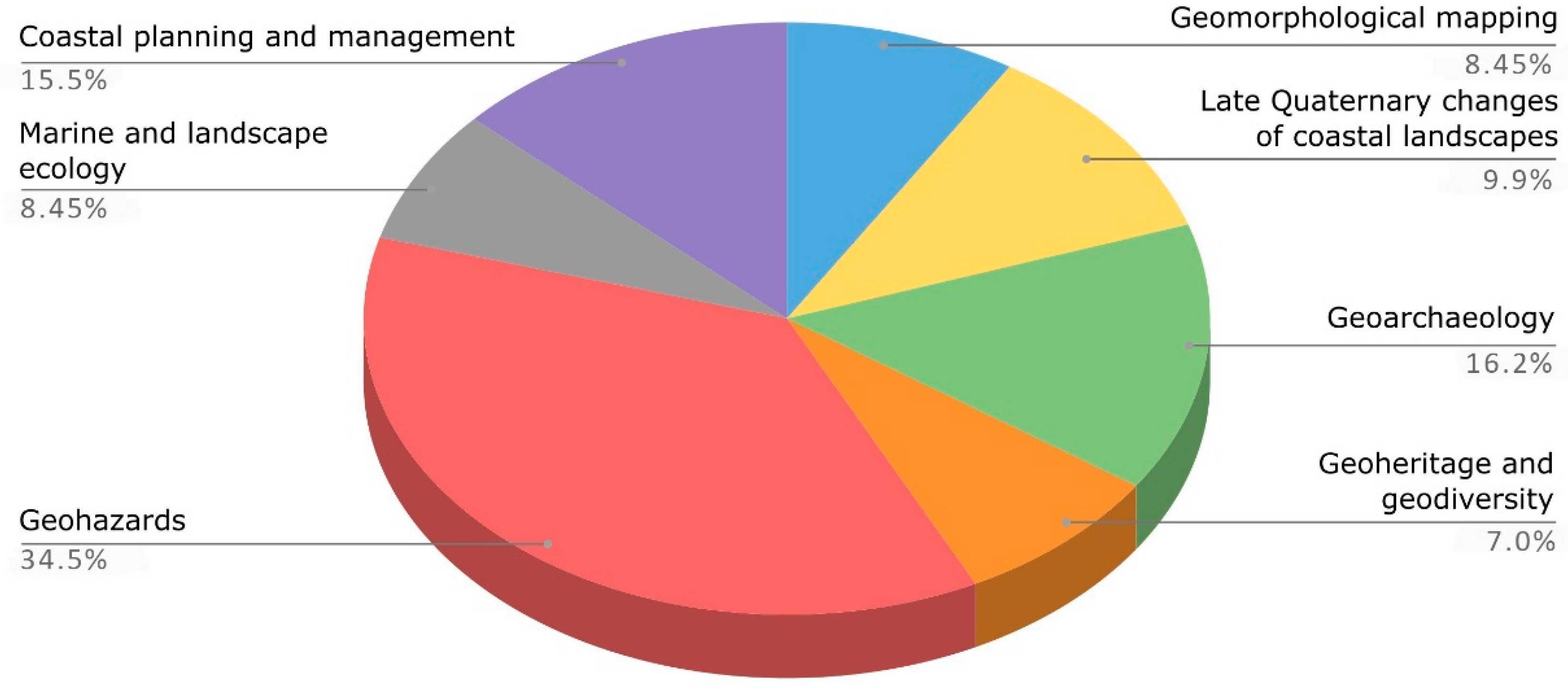
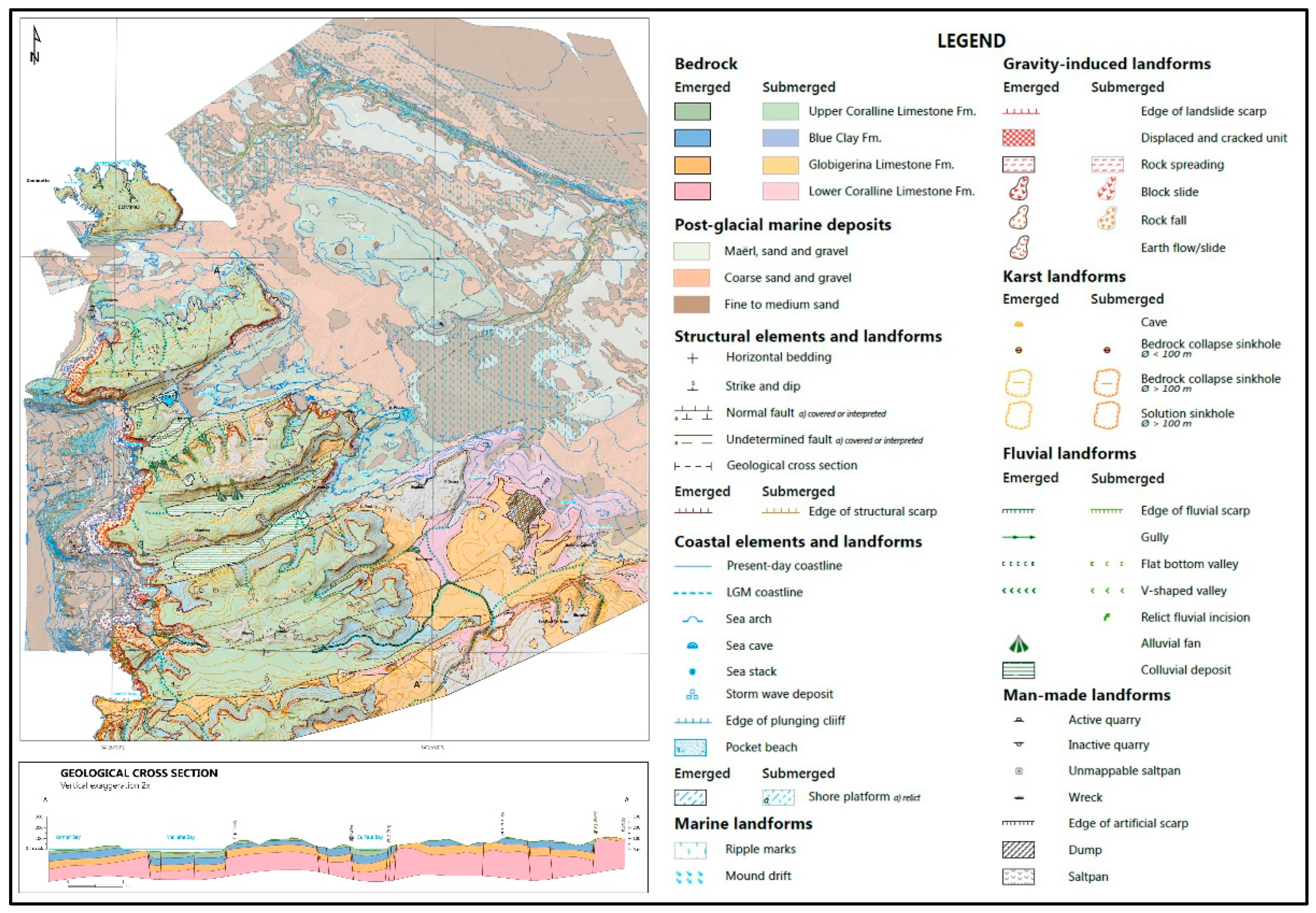
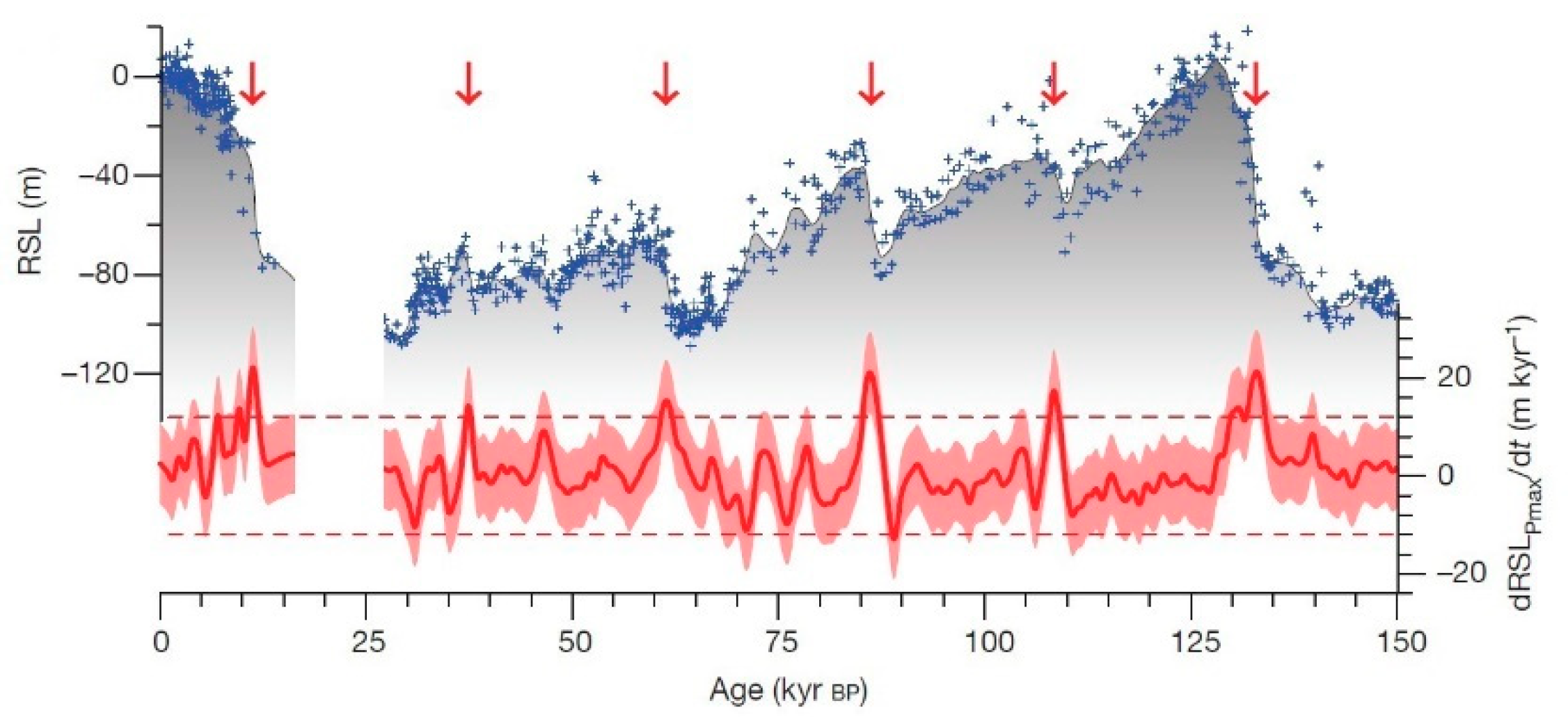
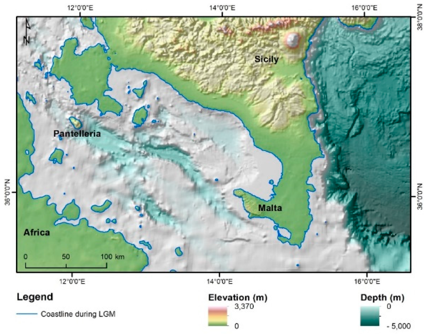
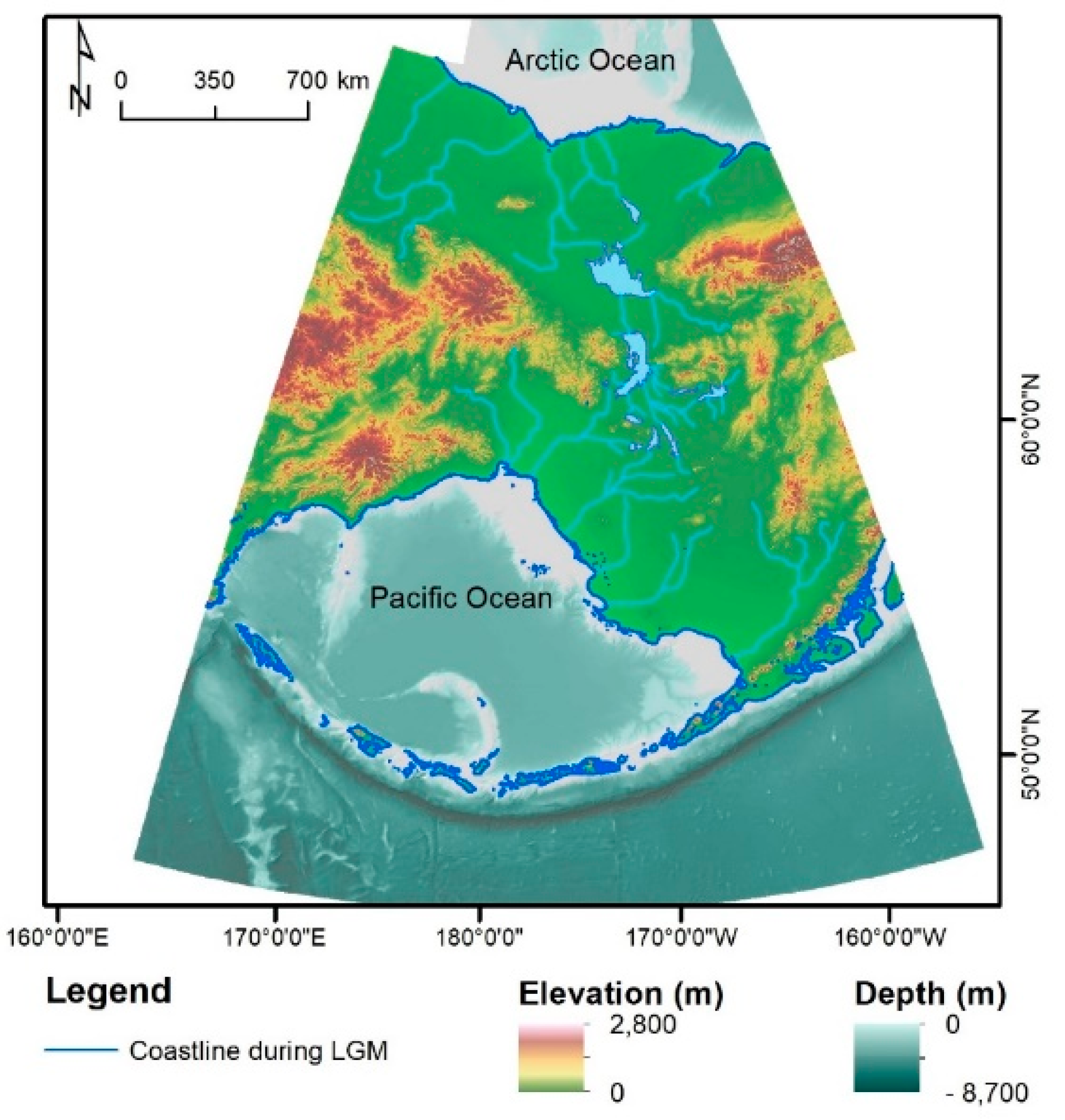
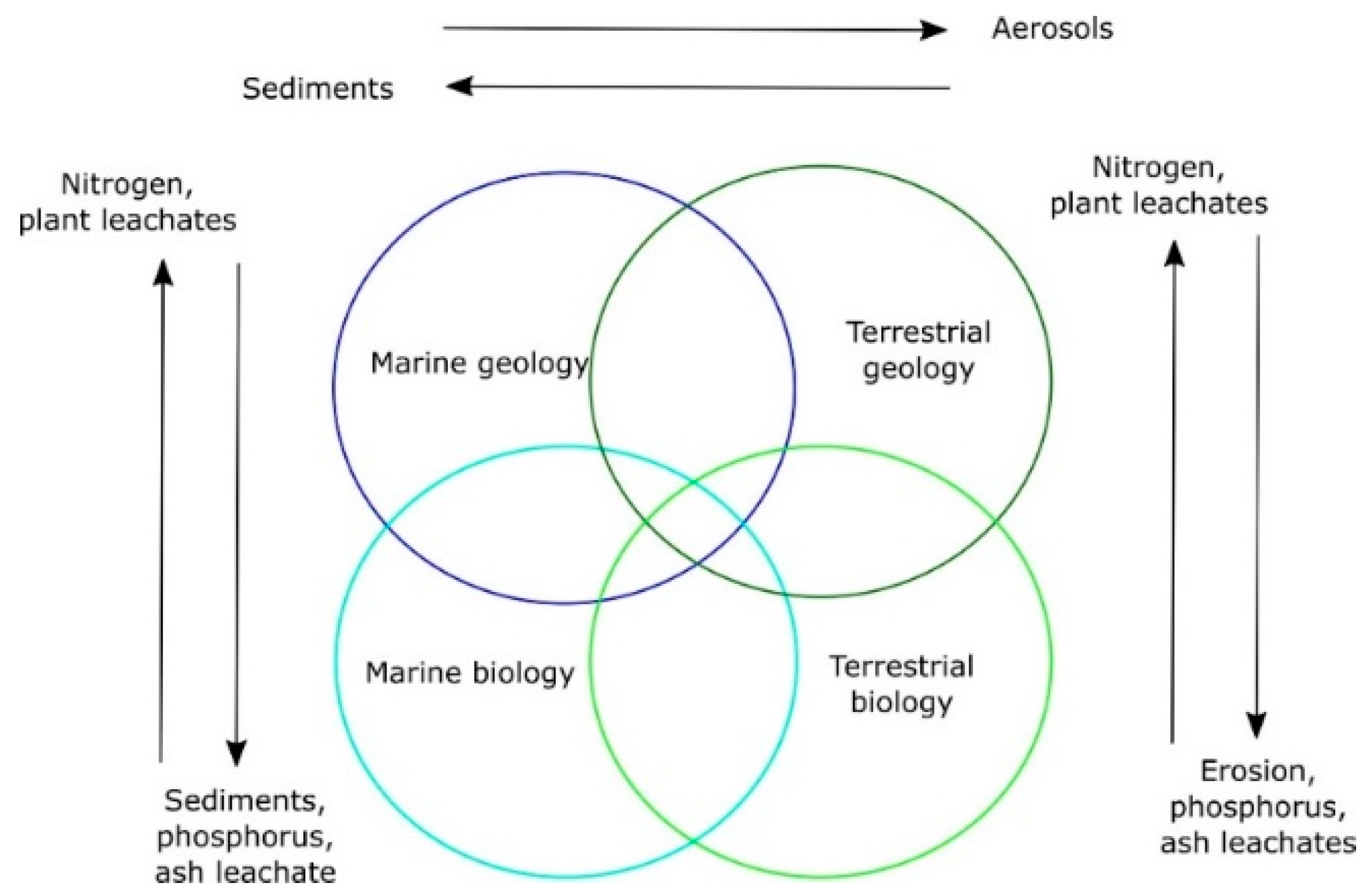
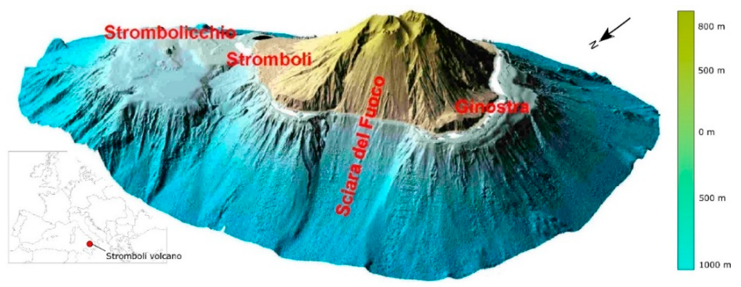
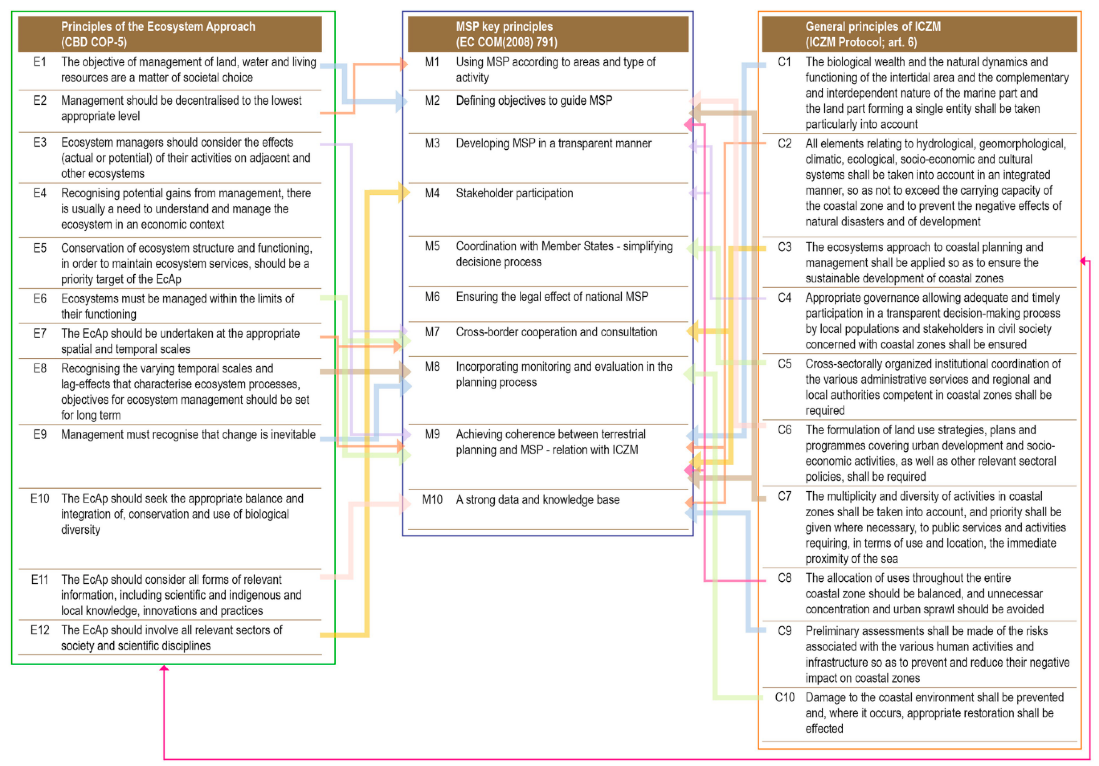
Table 1.
Outline of the most relevant scientific literature showing the outputs of integrated terrestrial and marine research with reference to the ‘seven good reasons’ mentioned above.
Table 1.
Outline of the most relevant scientific literature showing the outputs of integrated terrestrial and marine research with reference to the ‘seven good reasons’ mentioned above.
| Field of Applications | Relevant Examples | |
|---|---|---|
| 1 | Geomorphological mapping | Miccadei et al. [18,19,20]; Leon et al. [21]; Gasparo Morticelli et al. [22]; Mastronuzzi et al. [23]; Prampolini et al. [6,24]; Brandolini et al. [25]; Furlani et al. [26]; Campobasso et al. [27]; Genchi et al. [28] |
| 2 | Late-Quaternary changes of coastal landscapes | Bridgland et al. [29]; Pujol et al. [30]; Rovere et al. [31]; Westley et al. [32]; Micallef et al. [33]; Kennedy et al. [34]; Greenwood et al. [35]; Aucelli et al. [36]; Foglini et al. [37]; Benjamin et al. [38]; Furlani et al. [39]; Furlani and Martin [40]; De Gioiosa et al. [41]; Lo Presti et al. [42] |
| 3 | Geoarchaeology | Antonioli et al. [43]; Bailey and Flemming [44]; Harff and Lüth [45,46]; Fisher et al. [47]; Benjamin et al. [48]; Westley et al. [32]; Bailey et al. [49]; Furlani et al. [50]; Anzidei et al. [51]; Evans et al. [52]; Westley et al. [53]; Bailey et al. [54]; Aucelli et al. [36,55]; Harff et al. [56]; Cawthra et al. [57]; Benjamin et al. [38]; Benjamin et al. [58]; Furlani and Martin [40]; Mattei et al. [59]; Sturt et al. [60]; Veth et al. [61] |
| 4 | Geoheritage and geodiversity | Orrù and Ulzega [62]; Orrù et al. [63,64]; Brooks et al. [65]; Rovere et al. [66]; Mansini Maia and Alencar Castro [67]; Veloo [68]; Gordon et al. [69,70]; Coratza et al. [71] |
| 5 | Geohazards | Moore et al. [72]; Mulder et al. [73]; Assier-Rzadkiewicz et al. [74]; Caplan-Auerbach et al. [75]; Gee et al. [76]; Masson et al. [77]; McMurtry et al. [78]; Zhang et al. [79]; Dan et al. [80]; Scheffers and Scheffers [81]; Chiocci et al. [82]; Baldi et al. [83]; Parrott et al. [84]; Casalbore [85]; Violante [86]; De Blasio and Mazzanti [87]; De Gange et al. [88]; Sultan et al. [89]; Casalbore et al. [90,91]; Chiocci and Ridente [92]; Lambeck et al. [93]; Mazzanti and Bozzano [94]; De Jongh and van Opstal [95]; Della Seta et al. [96]; Knight and Harrison [97]; Masselink and Russel [98]; Mastronuzzi et al. [99]; Minelli et al. [100]; Carracedo [101]; Cazenave et al. [102]; Mataspaud et al. [103]; Mottershead et al. [104]; Biolchi et al. [105]; Yonggang et al. [106]; Antonioli et al. [107]; Aucelli et al., [108]; Zaggia et al. [109]; Casalbore et al. [110]; Di Paola et al. [111]; Moore et al. [112]; Obrocki et al. [113]; Pennetta et al. [114]; Urlaub et al. [115]; Biolchi et al. [116]; Buosi et al. [117]; Mucerino et al. [118]; Toker et al. [119]; Rizzo et al. [120] |
| 6 | Marine and landscape ecology | Hogrefe et al. [121]; McKean et al. [122,123]; Tallis et al. [124]; Wright and Heyman [12]; Vierling et al. [125]; Brown et al. [126]; Leon et al. [21]; Marchese et al. [127]; Prampolini et al. [6,128]; Harris and Baker [129] |
| 7 | Coastal planning and management | Cicin-Sain and Belfiore [130]; Sarda et al. [131]; Schultz-Zehden et al. [132]; Cogan et al. [133]; Ehler et al. [134]; Watts et al. [135]; Meiner [136]; Schlacke et al. [137]; Smith et al. [138]; Qiu and Jones [139]; Kerr et al. [140]; Ramieri et al. [141,142]; Barbanti et al. [143]; Domínguez-Tejo et al. [144]; UNEP/MAP [145]; UNEP-MAP PAP/RAC [146]; Decision IG. 22/1 [147]; Decision IG. 22/2 [148]; Sustainable Development Goals [149,150]; UNEP/MAP PAP [151] |
Table 2.
List of sensors and techniques cited in the text which are relevant for collecting elevation data in the shallow-water environment (i.e., white ribbon). Active sensors are those sensors that control the projection of acoustic or electromagnetic waves (i.e., sound or light) onto the scene, while the term “passive” refers to those systems or techniques that use ambient light to illuminate the scene or techniques such as Structure from Motion (SfM). MBES: Multi-Beam Echo-Sounder; PDBS: Phase Differencing Bathymetric Systems; MPES: multi-phase echo-sounders; ASV: Autonomous Surface Vessels; USV: Uncrewed surface vehicles; ROV: Remotely Operated Vehicle; UAV: Uncrewed Aerial Vehicle; LiDAR: Light Detecting And Ranging; LLS: Laser Line Scanning; SDB: Satellite-Derived Bathymetry; SfM: Structure from Motion.
| Active Sensors | ||||
|---|---|---|---|---|
| Sensor | Platform | Achievable DTM Resolution (Nearshore) | Survey Environment | |
| Acoustic | MBES (beamforming) | Vessel ASV/USV ROV | Sub-metric | Water |
| PDBS (Interferometers) | ||||
| MPES (Hybrid) | ||||
PROS:
| CONS:
| |||
| Optical | Bathymetric LiDAR | Airborne UAV | Sub-metric | Air/water |
PROS:
| CONS:
| |||
| LLS | Vessel ROV | Sub-metric | Water | |
PROS:
| CONS:
| |||
| Passive Sensors and Computational Techniques | ||||
| Name | Platform | DTM Resolution (Nearshore) | Survey Environment | |
| Optical | SDB | Satellite | 2 m | Air/Water |
PROS:
| CONS:
| |||
| SfM | UAV | Sub-metric | Air/Water | |
PROS:
| CONS:
| |||
© 2020 by the authors. Licensee MDPI, Basel, Switzerland. This article is an open access article distributed under the terms and conditions of the Creative Commons Attribution (CC BY) license (http://creativecommons.org/licenses/by/4.0/).
Share and Cite
MDPI and ACS Style
Prampolini, M.; Savini, A.; Foglini, F.; Soldati, M. Seven Good Reasons for Integrating Terrestrial and Marine Spatial Datasets in Changing Environments. Water 2020, 12, 2221. https://doi.org/10.3390/w12082221
AMA Style
Prampolini M, Savini A, Foglini F, Soldati M. Seven Good Reasons for Integrating Terrestrial and Marine Spatial Datasets in Changing Environments. Water. 2020; 12(8):2221. https://doi.org/10.3390/w12082221
Chicago/Turabian StylePrampolini, Mariacristina, Alessandra Savini, Federica Foglini, and Mauro Soldati. 2020. "Seven Good Reasons for Integrating Terrestrial and Marine Spatial Datasets in Changing Environments" Water 12, no. 8: 2221. https://doi.org/10.3390/w12082221
Note that from the first issue of 2016, this journal uses article numbers instead of page numbers. See further details here.