An Improved Immersed Boundary Method for Simulating Flow Hydrodynamics in Streams with Complex Terrains


1
Department of Civil and Environment Engineering, Pennsylvania State University, University Park, PA 16802, USA
2
Technical Service Center, U.S. Bureau of Reclamation, P.O. Box 25007, Denver, CO 80225, USA
3
Department of Civil and Environment Engineering, Institute of Computational and Data Sciences, Pennsylvania State University, University Park, PA 16802, USA
*
Author to whom correspondence should be addressed.
Water 2020, 12(8), 2226; https://doi.org/10.3390/w12082226
Submission received: 16 July 2020
/
Revised: 3 August 2020
/
Accepted: 5 August 2020
/
Published: 7 August 2020
(This article belongs to the Special Issue Multi-Dimensional Modeling of Flow and Sediment Transport)
Abstract
:Three-dimensional (3D) computational fluid dynamic (CFD) simulations have gained substantial popularity in recent years for stream flow modelling. The complex terrain in streams is usually represented by a 3D mesh conforming to the terrain geometry. Such terrain-conforming meshes are time-consuming to generate. In this work, an immersed boundary method is developed in an existing terrain-conforming CFD model named U2RANS as an alternative, in which terrains are represented implicitly in the Cartesian background mesh. An improved two-layer wall function is proposed in the framework of the k-ε turbulence model, with the aim of producing accurate and smooth wall shear stress distribution and paving the way for future model development on sediment transport and scour modeling. The improvement overcomes the inherent discontinuity and nonlinearity of the two-layer velocity profile, which causes error in the estimation of shear velocity. The new algorithm utilizes a distance control on the image point in immersed boundary method and a modification of velocity prediction in the laminar layer. The improved immersed boundary method is tested with 1D, 2D, and 3D cases, and comparisons with flume experiments show promising results.
1. Introduction
Traditional three-dimensional (3D) modeling requires a 3D mesh to conform to domain geometry, termed the “terrain-conforming method” in this paper. Despite the widespread use of the terrain-conforming method in Computational Fluid Dynamics (CFD) models, generation of a high-quality mesh is still a challenging task in 3D modeling of flows over complex terrain. A very refined near-wall mesh must be used to resolve the boundary layer to produce an accurate solution. The stability and accuracy of the terrain-conforming method highly depend on the mesh quality. In addition, the mesh size increases rapidly with the increase of Reynolds numbers [1].
In this work, we aim to present a user-friendly 3D CFD model for practical applications in hydraulic engineering. An alternative way to the terrain-conforming method is the immersed boundary (IB) method, in which terrains are embedded in a background mesh. The boundary conditions on terrain surface are implicitly represented by modifying the governing equations of the flow. Such a method is also referred to as the terrain-embedding method in this work. Special numerical treatments are developed to implement the solid boundary conditions for turbulent flows near complex terrain and solid objects. For example, a discrete-forcing term can be added in the discretized Navier-Stokes equations to represent the embedded terrain [2,3]. The forcing term is calculated from the no-slip condition and the moving velocity of the immersed surface if the boundary motion is considered. This method is referred to as the Kinematic IB scheme [4].
With the IB method, mesh generation becomes relatively simple, as only a background mesh is needed, and mesh quality is easy to control. A key issue of the IB method is the model accuracy in simulating turbulent flows, although it has been demonstrated for laminar flows. Another advantage of the IB method is that it can easily track terrain deformation, which is important in the simulation of sediment transport and scour. With the terrain-conforming methods, the mesh has to be regenerated to conform to the terrain or solid body movement in each morphological time step. The mesh regeneration is difficult to perform and may lead to numerical instability and loss of accuracy due to the deterioration of the mesh quality caused by large movement. With the IB method, terrain deformation is captured by recalculating the discrete-forcing term and no mesh changes are necessary.
A key variable in sediment transport and scour simulation is the wall shear stress on erodible beds. Existing algorithms of the IB method have demonstrated good performance in the prediction of flow velocity [5,6]. However, the accuracy and smoothness of the wall shear stress in the IB method need improvements. This issue is mainly caused by the poor prediction of the velocity profile between the near-wall cell and the terrain boundary [7]. The other reason is the mass conservation problem on the terrain boundary [7]. In addition, the implementation of a wall function in the IB method is a significant challenge, especially for high Reynolds number flows. To avoid high mesh resolution in the near-wall region, attempts have been made in the implementation of wall models in the large eddy simulation (LES) framework [8,9]. For example, Roman et al. proposed a Reynolds-Averaged Navier-Stokes (RANS)-like eddy viscosity to reconstruct the wall shear stress in LES [8].
Considering that there are drastically different time scales in hydrodynamics and morphodynamics (the latter is much slower than the former) [10], a wall model in the RANS framework is more suitable for real-world applications. Tamaki et al. proposed a Spalart-Allmaras (SA) wall model using the IB method, and modified the eddy viscosity to balance the shear stress [11]. Capizzano adopted a two-layer wall model in the near-wall region for k-ω and k-g turbulence models with a blending estimation of and [12]. Zhou applied a blending of Spalding’s law, Reichardt’s law, and log-law in the SST k-ω turbulence model [13]. The key of the most existing wall functions is to avoid the transition of the wall model between the viscous sublayer and the log-law sublayer by either using the blending turbulence variables or using continuous velocity profiles.
Despite the progresses made in the IB methodology and its applications in river hydraulics, mature models are yet to be developed to have the accuracy, stability, and efficiency needed for real-world applications. In particular, a reliable sediment transport and scour model would hinge on the accurate prediction of the bed shear stress. In this work, we present an improved IB algorithm which is then implemented into the terrain-conforming model of [14] (named U2RANS). The aim is to develop an IB-method based 3D model so that accurate flow and bed shear stress may be predicted. This paper extends the work presented in [15,16]. Specifically, a two-layer wall function is implemented in association with the k-ε turbulence model [17] and the IB method. The model is then verified to produce an accurate velocity field, as well as a smooth and accurate wall shear stress distribution. A key contribution of the present study is the improvement of the model accuracy through the control of the image point position, which is a point used in the IB model to reconstruct the near-wall flow field. In addition, a modification of the wall model in the laminar sublayer allows better handling of the discontinuity between the viscous sublayer and the logarithmic layer. As a result, a better estimation of wall shear stress can be achieved.
The new IB-method-based U2RANS model is validated and demonstrated using a number of flow cases in the following. As discussed before, due to the limitations of the terrain-conforming method, the terrain-embedding method is more suitable for modeling of real-world cases, particularly for sediment transport and scour modeling. The scour modeling is under development and will be reported in the future.
2. Numerical Methods
U2RANS is a 3D CFD model using the unstructured mesh with arbitrarily shaped cells [14]. The flow is assumed incompressible, viscous, and Newtonian. The governing RANS equations are as follows:
where is time; is the flow density; is the mean velocity; is the turbulence stress; is the mean pressure; is the kinematic viscosity; and is the gravity acceleration.
The Reynolds stress tensor is calculated with the standard k-ε model of [17]:
where is the Kronecker delta (a unit tensor) and the eddy viscosity is calculated as:
where ; is the turbulence kinetic energy; and is the turbulence dissipation rate.
The transport equations for and are:
where is the turbulence generation rate; ; ; ; and .
A numerical solution to the above flow equations involves the use of a mesh to cover the model domain, followed by discretization of the governing equations. With the IB method, only a background mesh is needed. The background mesh itself, however, can be unstructured and assume polyhedral shapes. Such a mesh is the most flexible and has the advantage of uniting various mesh topologies into a single formulation. The cell-centered scheme is adopted with all dependent variables located at the centroid of a mesh cell. The other alternatives include the cell-vertex scheme, with which all variables are at the cell’s vertices, or a staggered scheme, with which the velocity and pressure are stored at difference locations. The governing equations are discretized using the finite-volume approach using the Gauss theorem. An advantage of the finite-volume method is that the conservation of any flow property can be achieved locally and globally. The detailed numerical method was referred to in [14], is and not repeated herein.
3. Immersed Boundary Implementation
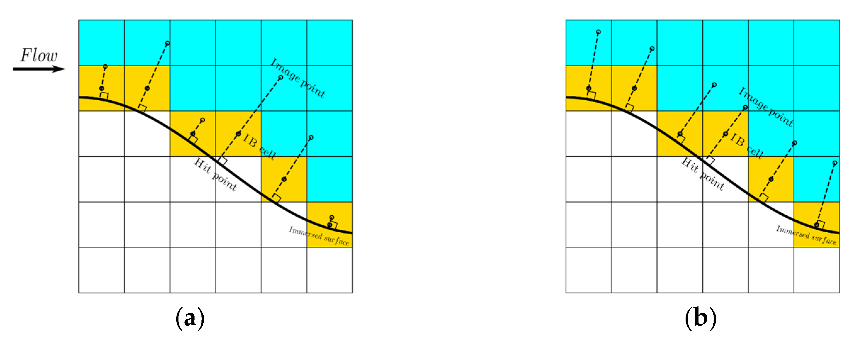
The proposed IB method uses a discrete forcing approach, where the forcing term is cell-based for an unstructured mesh. The IB cells are cells cut by the immersed surface, and their cell centers are located on the fluid side (yellow cells shown in Figure 1). Three different points are identified: (1) the IB cell center (IB); (2) the hit point (HP), which is the intersection of the immersed surface with its normal line through the cell center; and (3) the image point (IP), which is the point on the extended line of the normal vector through the cell center in the fluid field. Three different characteristic lengths are identified: (1) wall distance : the distance from the IB cell center to the corresponding hit point; (2) image distance : the distance from the image point to the corresponding hit point; (3) and IB cell length : the minimum dimension of all IB cells. To enforce the turbulence model conditions at the IB cell centers, the following steps are carried out:
- The tangential flow velocity at an image point is reconstructed by using a distance-based weighting procedure with the neighboring cells around the image point.
- Based on the log-law velocity profile, the dimensionless distance and are computed (iteratively) as:where and .
- The shear velocity on the immersed surface is calculated as:
- The tangential flow velocity , , and at the IB cell center are calculated based on :where and . The implementation of and are similar to the wall functions for and used in OpenFOAM [18].
- Fix the values of flow variables on the IB cell centers when solving the momentum equation and the transport equations for and .
- Adjust the flux balance on the faces of IB cell centers on the solid side for mass conservation.
The key to the IB treatment is the estimation of the shear velocity , that is, the calculation of . Considering the nonlinear and discontinuous nature of velocity profile between the laminar sublayer and log-law sublayer, the result of converges to different values if different velocity profiles are used. To keep the consistency when estimating the shear velocity of all IB cells, Equation (7) assumes that the image points are located within the log-law sublayer such that only the log-law velocity profile is used in the iteration. Generally, the image point distance is proportional to the wall distance (for example, = 3), as shown in Figure 1a [19,20]. However, the wall distance is arbitrarily distributed around the immersed surface, making it impossible to guarantee that the image point is located in the logarithmic sublayer. In addition, an extremely small value of may result in numerical instability and even divergence of the model. In this work, is set to be proportional to the minimum dimension of each IB cell = 3). Consequently, the image points are uniformly distributed along the immersed surface, as shown in Figure 1b. The numerical instability due to the small value of is avoided. A similar implementation has been used in [12] and [11] for the k-ω model and SA model.
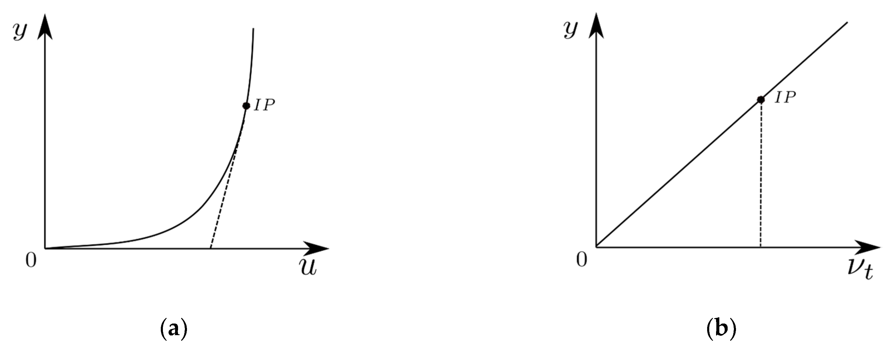
Another problem in the near-wall treatment of the immersed boundary method comes from the inconsistency when the IB cell center and its corresponding image point are located in different sublayers of the velocity profile. Although all image points are designed to be in the log-law layer, the wall distance is still an arbitrary value and the IB cell center may be in the laminar sublayer. Therefore, Equation (9), which assumes the IB cell center and its image point follow the same logarithmic velocity profile, is not applicable in this situation. To address this problem, a modified velocity profile is used when the IB cell center is in the laminar sublayer. We assume a linear velocity profile between the wall and the image point, such that the first derivative of the velocity with respect to the wall distance is still a constant (Figure 2a). This method was proposed in [11] to correct the mass flux on the cell boundary by using a slip velocity boundary condition. Here, it is used to extend the logarithmic velocity profile to the wall when the IB cell center is in the laminar sublayer. The eddy viscosity is also modified to be a constant between the wall and the image point (Figure 2b). Thus, , and are constant in this region. This modification is based on the balance of shear stress on the boundary:
The modified flow velocity , , and at the IB cell center are calculated as the following:
where In the following, this is called the modified wall model, and the one presented before is called the original model.
4. Result
The above IB method is implemented into the U2RANS model. In this section, a number of turbulent flow cases are selected to verify the improved IB method. In particular, model accuracy is examined and discussed.
4.1. Turbulent Flow over Flat Plate
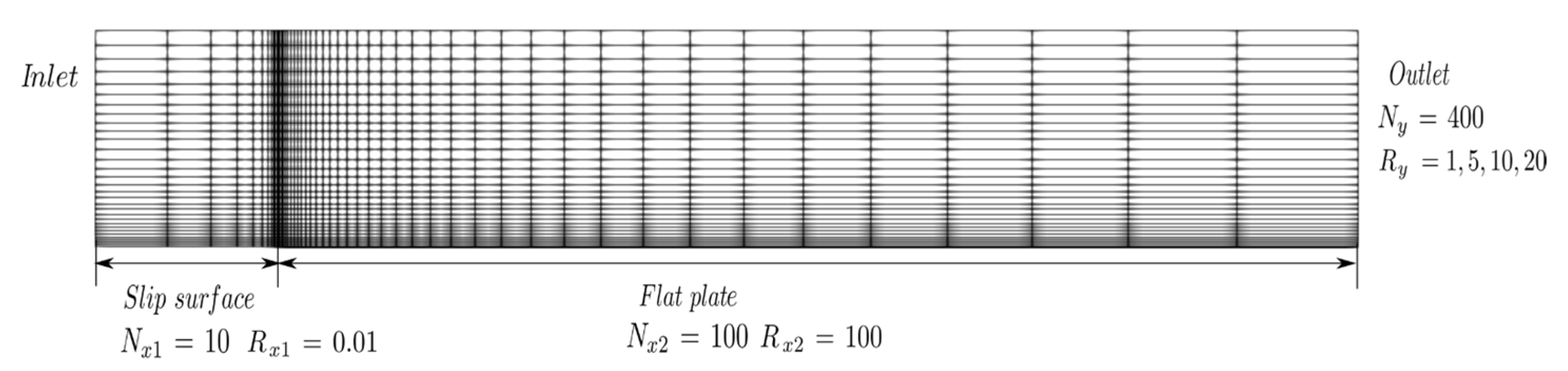
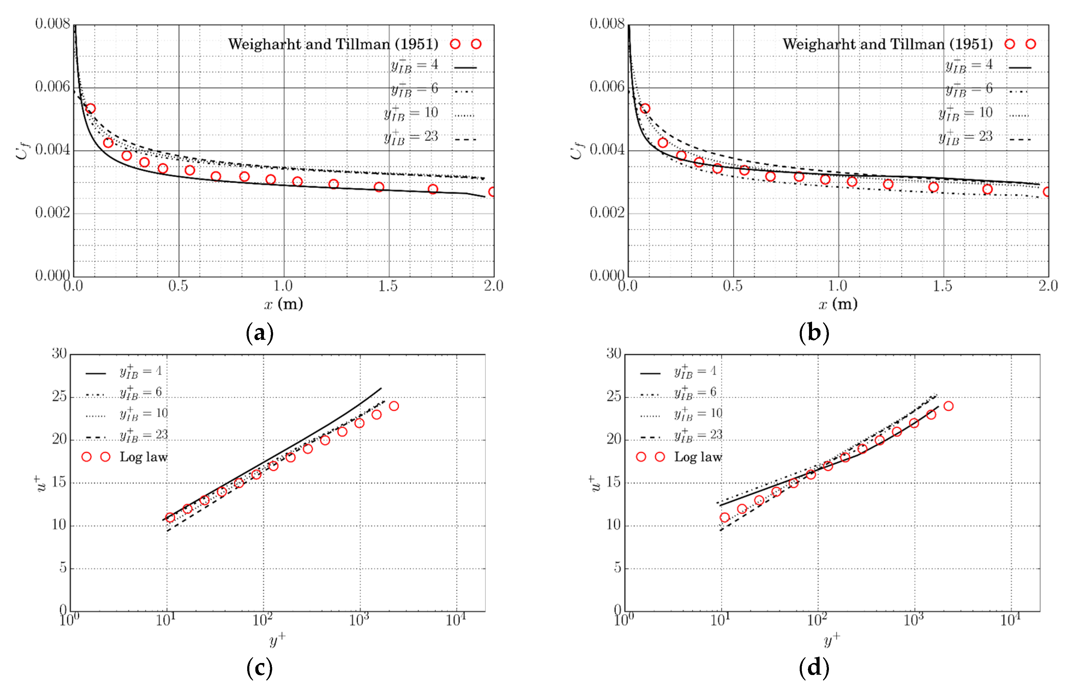
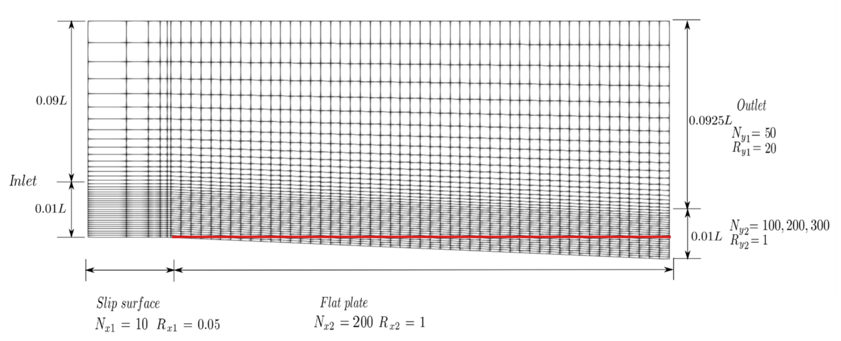
The flow over a flat plate was used to investigate a 2D boundary layer without pressure gradient. The case is used to verify the IB method implementation with the proposed wall function. The length L of the plate is 2 m. The Reynolds number based on the plate length is and incoming flow velocity is = 2.5 m/s. The upper boundary is 0.1L away from the flat plate. The Cartesian mesh is refined near the leading edge and the plate. The mesh arrangement is shown in Figure 3. A short slip surface (0.1L) is added in front of the leading edge using the symmetric boundary condition. The flat plate is modeled as an immersed boundary, and the wall boundary condition is applied on it. We tested four different mesh sizes by using four different cell expansion ratios, , in the y-direction to change the mesh size of the first cell touching the wall. The cell expansion ratio, , is that of the size of the end cell to the size of the start cell along the edge direction (). Different mesh sizes change the value of and . For both original and modified wall models, the computed local friction coefficient () along the plate compares well with the experimental data from [21] (Figure 4a,b); the velocity profiles at 0.9L are in good agreement with the log-law (Figure 4c,d). In addition, as decreases, the simulation results converge to the experimental data. The results show that the proposed IB algorithm with an original or modified wall model is insensitive to the image point distance in the log-law layer.
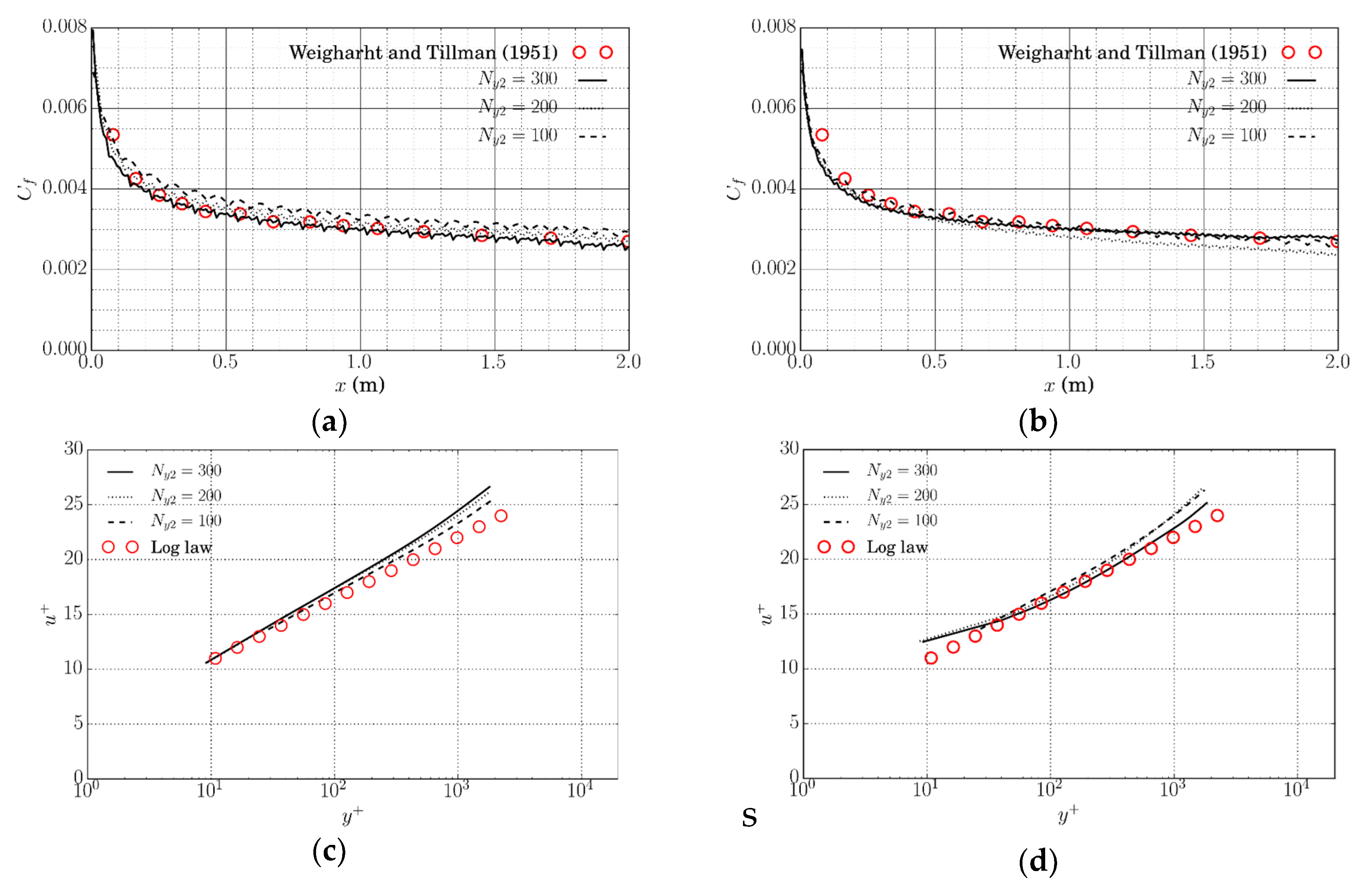
To further investigate the stability of the algorithm and its dependence on wall distance, the mesh above the flat plate is rotated, as shown in Figure 5. The top line of the grid has the same height to maintain the same water depth throughout the length. The bottom of the mesh is rotated, and the downstream end of the bottom is moved down by 0.0025L. The red line represents the position of the flat plate. With this configuration, the mesh lines are not aligned with the flat plate. As the grid rotates (stretches), the wall distance is not uniformly distributed along the plate. Other details of the mesh arrangement are shown in Figure 5. is the number of mesh refinement in the y-direction used in the region between the bottom line and the line 0.1L away from the bottom. We changed the number of () to show the mesh independence of this method. The cell expansion ratio in the y-direction in the refinement zone is 1 to maintain the minimum dimension constant for each IB cell, such that the image point distance is the same; but the wall distance distribution is nonuniform over the plate. Figure 6a shows the numerical results of the local friction coefficient using the original wall model. The predicted results are comparable with the experiment. However, there are some small, semi-periodic oscillations due to the change of wall distance along the plate, especially when the value of decreases and the IB cell center is in the laminar sublayer. To suppress the oscillation from the nonuniform wall distance, the modified wall model is applied and the simulated results are plotted in Figure 6b. The modified wall model can predict the local friction coefficient more accurately and the oscillation is greatly reduced. As the mesh is refined, the local friction coefficient converges to the experimental data. In addition, velocity profiles in Figure 6b and d at 0.9L agree well with the log-law. Both the original and modified wall models give a good prediction of velocity.
Table 1 provides the computational cost in one iteration of the IB method with the modified wall model. The calculation of the modified wall model includes the finding of IB cells, identification of image stencil for reconstruction, and implementation of wall function. All simulations were performed on a Dell Precision Tower 5810 with an Intel Xeon CPU ES-1620. The computational cost of the modified wall model is about 60% of the total CPU time in one iteration for each case. However, considering the boundary is immobile in this work, the IB cells and image stencil are only calculated in the first iteration, and remain unchanged in the following iterations. The percentage of the computational cost of the modified wall model greatly decreases over the whole simulation time. In addition, the modified wall model avoids the computational cost required to fully resolve the near-wall flow in the laminar layer.
4.2. Turbulent Flow around a Cylinder over Scoured Beds
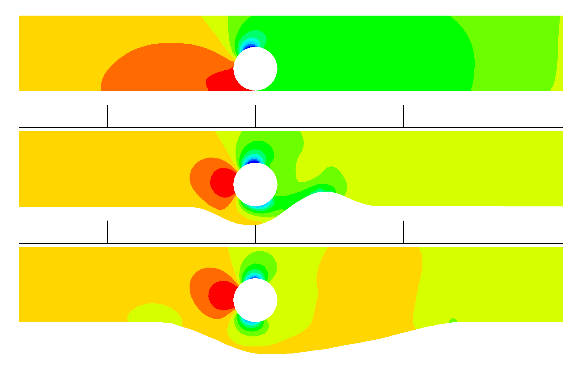
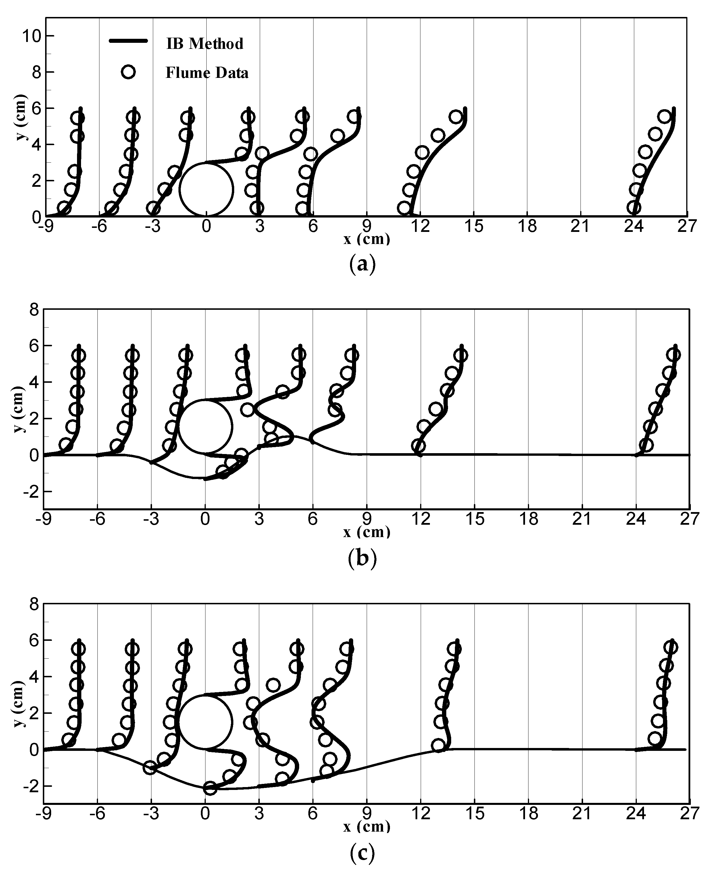
The proposed IB algorithm is verified next for its capability to simulate a case with an instream structure—a turbulent flow around an instream cylinder over scoured beds. The modified wall model is used. The simulated results are compared with the flume experiment by Jensen et al. [22]. Figure 7 shows the three bed profiles representing three scour phases observed in the experiment by Mao [23]. The cylinder has a diameter of 3 cm and is placed above three scoured bed profiles. The mean inlet flow velocity is 0.2 m/s. The computational domain is 1.1 m in the streamwise direction (x-direction). The flow depth at the uneroded bed at the exit is maintained at 0.245 m (y-direction). Despite 2D flow in nature, the modeling is carried out in a 3D model domain with the dimension of 0.03 m along the cylinder (z-direction).
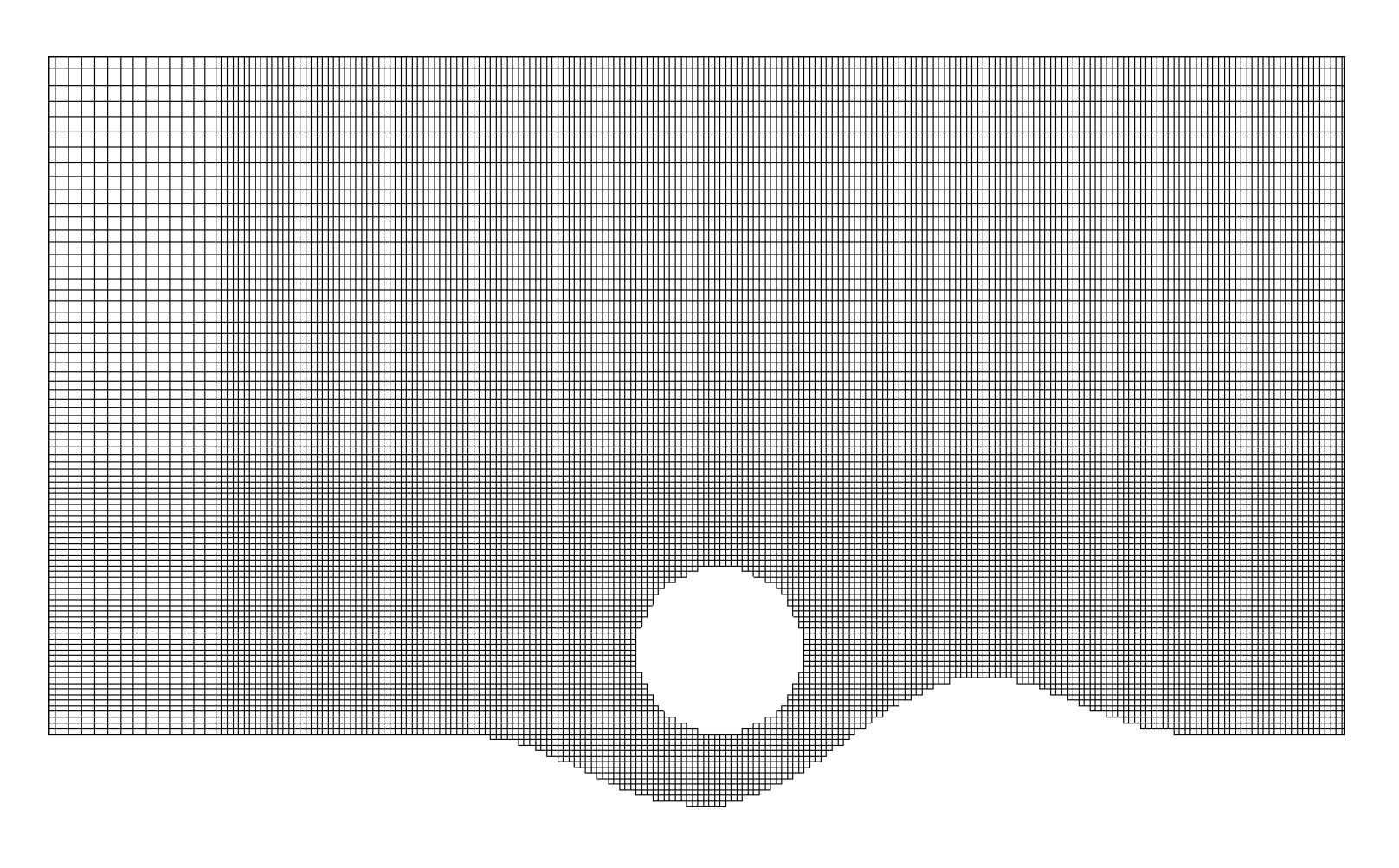
Using profile 3 as an example, the Cartesian background mesh has 0.1 cm resolution near the cylinder and scour bed, which is the finest resolution similarly used by Smith and Foster [24]. The background mesh has a total of 355,515 3D cells (71,103 2D cells in the xy plane and 5 cells along z). The cylinder boundary and bed profiles are treated as the immersed boundaries. The fluid and IB cells near the immersed boundaries are shown in Figure 8. The meshes for the two other profiles are similar.
Figure 9 shows the comparisons between simulation results and measured data from experiments. It is seen that the computed streamwise (x) velocity profile approaching the cylinder is near-logarithmic, although a constant velocity boundary condition is applied at the inlet. The IB method-simulated velocity profiles agree well with the experimental data for all three profiles and at the eight streamwise stations. The results show that the recovery from the cylinder is slow, even at the last measured location about eight cylinder diameters downstream (x = 24 cm) where the wake effect of the cylinder is still significant.
4.3. Turbulent Flow over 3D Dunes
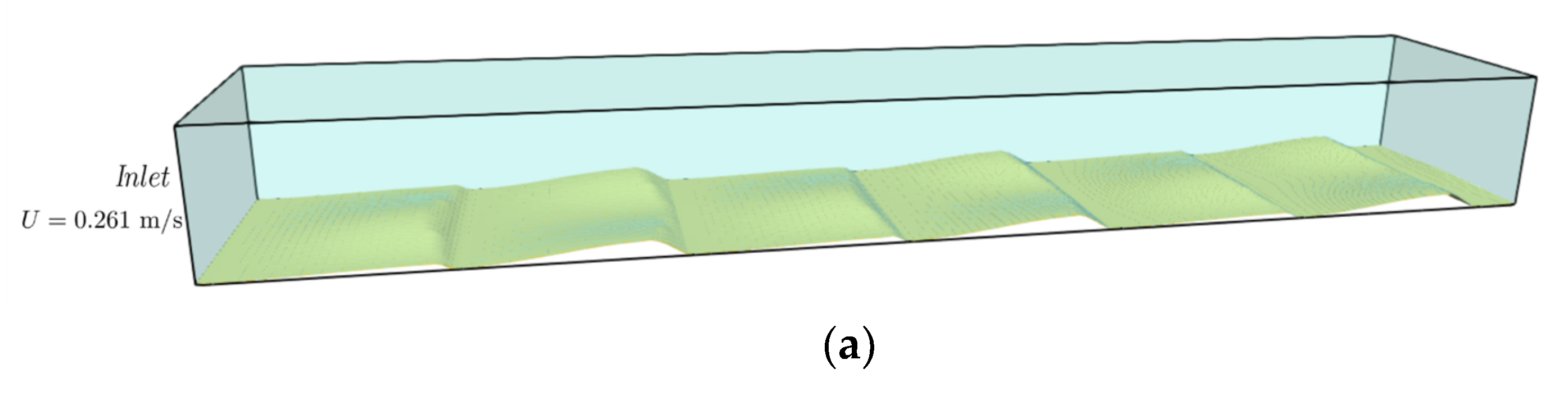
3D dunes were used to verify the model performance with the turbulence model in a 3D form, especially the prediction of wall shear stress. The modified wall model is used in this case for a more accurate and smooth wall shear prediction. The simulation results are compared with the experiments of [25]. In the experiment, 14 fixed 3D dunes were placed on the bottom of the flume sequentially and experimental data were measured on the 11th and 12th numbered dunes. Only six dunes were simulated to reduce the computational cost, and the data were collected from the last two dunes, as shown in Figure 10a. The length of the simulation domain is 5.0 m in the x-direction and the width of the domain is 0.9 m in the y-direction. The bed elevation contour of the 3D dunes is shown in Figure 10b. The incoming velocity is 0.261 m/s in the x-direction and the water depth is 0.561 m in the z-direction.
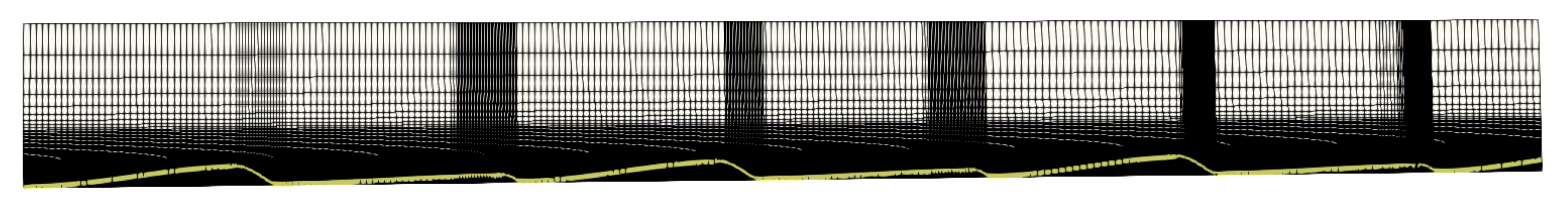
The Cartesian background mesh is shown in Figure 11. The numbers of cells are 450, 90, and 70 in the x, y, and z directions, respectively. The mesh is refined near the dunes, especially where the bed elevation changes rapidly.
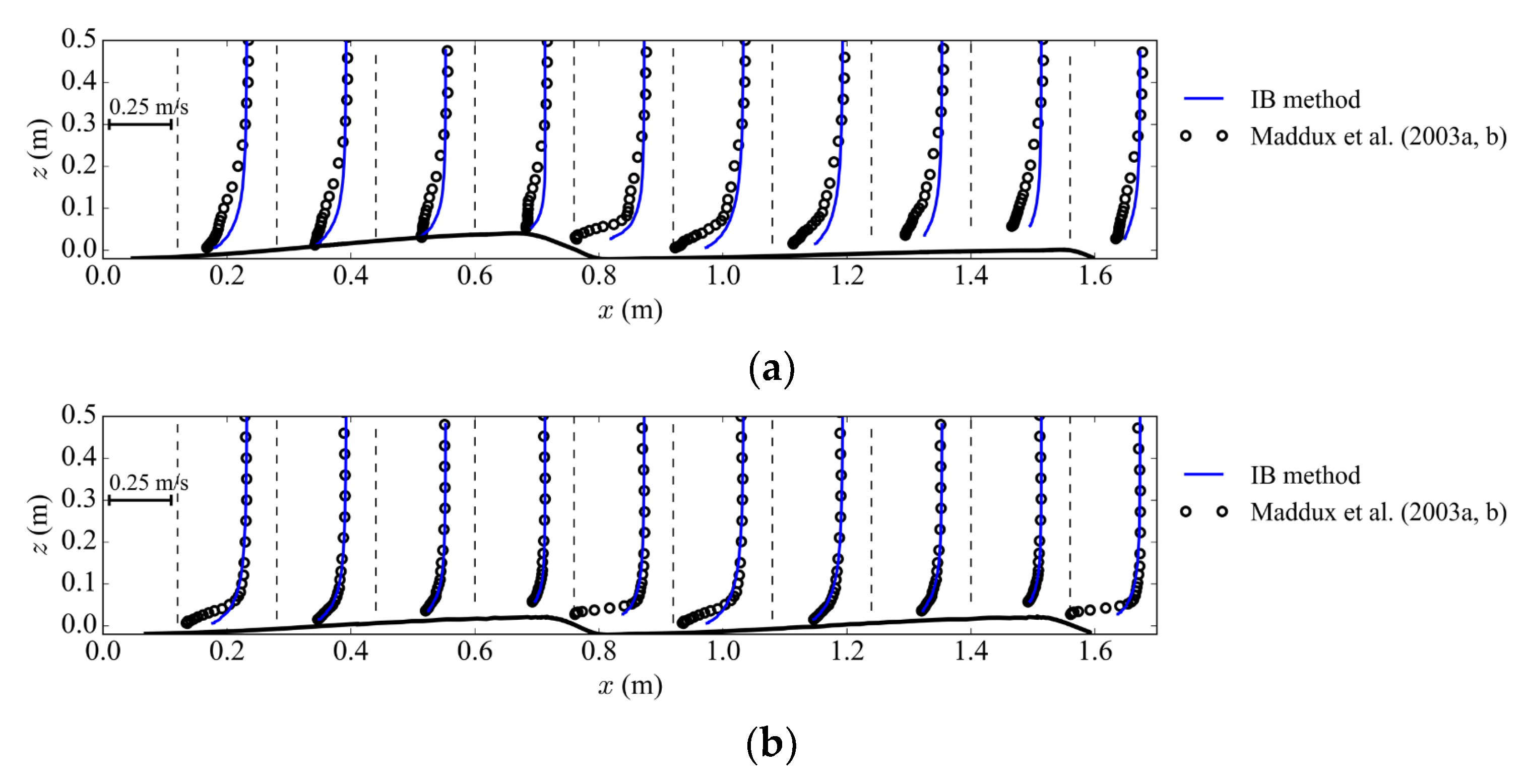
Figure 12 is a comparison of results from the IB method and the experiment. The streamwise velocities at different locations are well-predicted. The only noticeable deviation is downstream of the measured two dunes at y = 0 m. In this slice, the bed elevation has the largest slope, such that a long distance from the inlet is required for the flow to be fully developed. In the experiment, the measured dunes are the eleventh and twelfth. However, the measured dunes in the simulation are at the fifth and sixth, due to the limitation of computing capacity. Thus, the flow condition is slightly different.
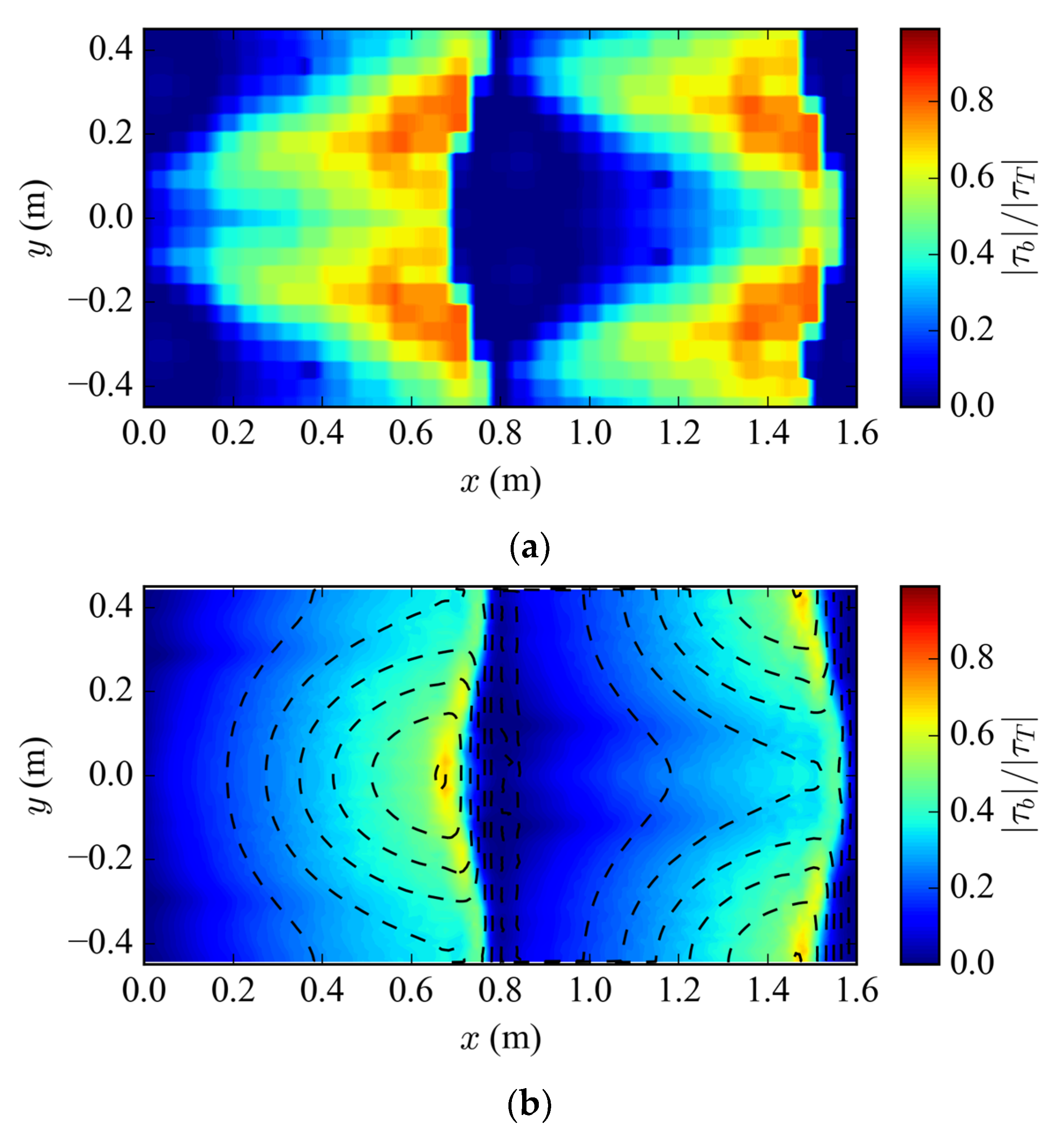
Comparison of bed shear stress is shown in Figure 13. The simulation results show that the new IB algorithm can provide a smooth wall shear stress distribution. The normalized wall shear stress of the measured data (Figure 13a) is estimated using the velocity 5 mm above the bed [25]:
where is the velocity at 5 mm above the bed, the distance is 5 mm, and mm is the bed roughness.
The wall shear stress from the IB simulation is based on Equations (7) and (8) and shown in Figure 13b. Even with the distribution of IB cells and image points changing arbitrarily with the bed elevation, the predicted shear stress is smooth. A comparison with the experimental data in Figure 13a shows the existence of mismatch between the two. This is mainly because the accuracy of the simulation is limited by the computing capacity, such that the velocity prediction at the places with large slope deviates from the experiment. However, the general characteristics of the wall shear stress are captured by the numerical model. The wall shear stress is the highest at the crests of dunes and relatively small elsewhere. The smooth distribution of wall shear stress is very important for modeling the sediment transport and scours, which is currently under development.
5. Conclusions
This work proposes a new wall model algorithm for use by the IB method in association with the k-ε turbulence model. It was implemented into the terrain-conforming U2RANS model of [14]. The aim was to develop a flexible IB-method-based CFD model so that turbulent flow field can be simulated accurately and smooth wall shear stress can be generated. A key contribution is to use a consistent velocity profile—log-law velocity profile—to estimate the wall shear velocity. In addition, a modification was proposed in the wall model for the laminar sublayer to suppress the oscillation caused by the small value of wall distance . In such a way, the discontinuity and nonlinearity of the velocity profile between the laminar sublayer and log-law sublayer are avoided. The proposed two-layer wall function has the same drawbacks of standard wall functions for non-equilibrium flow with a large pressure gradient, such as stagnation point and separated flow. However, it provides a relatively accurate prediction of a high Reynolds number and wall-bounded flow with an affordable computational cost. The new method was tested and validated with selected 1D, 2D, and 3D flow cases. Good results were obtained in each case. The proposed method produces an accurate and smooth wall shear stress distribution, paving the way for the next stage of model development for sediment transport and scour modeling.
Author Contributions
Conceptualization, Y.S. and X.L.; methodology, Y.S.; software, Y.S. and Y.G.L.; validation, Y.S. and Y.G.L.; writing—original draft preparation, Y.S.; writing—review and editing, Y.G.L. and X.L. All authors have read and agreed to the published version of the manuscript.
Funding
This research was funded by U.S. Bureau of Reclamation, grant number R17AC00025.
Acknowledgments
We thank the anonymous reviewers for their comments and suggestions.
Conflicts of Interest
Co-author Y.G.L. is an engineer working for the U.S. Bureau of Reclamation, who is the funder of this work.
References
- Mittal, R.; Iaccarino, G. Immersed boundary methods. Annu. Rev. Fluid Mech. 2005, 37, 239–261. [Google Scholar] [CrossRef] [Green Version]
- Mohd-Yusof, J. For simulations of flow in complex geometries. Annu. Res. Briefs 1997, 317, 35. [Google Scholar]
- Verzicco, R.; Mohd-Yusof, J.; Orlandi, P.; Haworth, D. LES in complex geometries using boundary body forces. In Proceedings of the Summer Program; Center for Turbulence Research: Stanford, CA, USA, 1998. [Google Scholar]
- Coclite, A.; Ranaldo, S.; de Tullio, M.D.; Decuzzi, P.; Pascazio, G. Kinematic and dynamic forcing strategies for predicting the transport of inertial capsules via a combined lattice Boltzmann–immersed boundary method. Comput. Fluids 2019, 180, 41–53. [Google Scholar] [CrossRef] [Green Version]
- Kim, J.; Kim, D.; Choi, H. An immersed-boundary finite-volume method for simulations of flow in complex geometries. J. Comput. Phys. 2001, 171, 132–150. [Google Scholar] [CrossRef]
- Tessicini, F.; Iaccarino, G.; Fatica, M.; Wang, M.; Verzicco, R. Wall modeling for large-eddy simulation using an immersed boundary method. In Annual Research Briefs; Center for Turbulence Research: Stanford, CA, USA, 2002; pp. 181–187. [Google Scholar]
- Harada, M.; Tamaki, Y.; Takahashi, Y.; Imamura, T. A Novel Simple Cut-Cell Method for Robust Flow Simulation on Cartesian Grids. In Proceedings of the 54th AIAA Aerospace Sciences Meeting, San Diego, CA, USA, 4–8 January 2016. [Google Scholar]
- Roman, F.; Napoli, E.; Milici, B.; Armenio, V. An improved immersed boundary method for curvilinear grids. Comput. Fluids 2009, 38, 1510–1527. [Google Scholar] [CrossRef]
- Yang, X.I.A.; Sadique, J.; Mittal, R.; Meneveau, C. Integral wall model for large eddy simulations of wall-bounded turbulent flows. Phys. Fluids 2015, 27, 025112. [Google Scholar] [CrossRef]
- Termini, D. Bed scouring downstream of hydraulic structures under steady flow conditions: Experimental analysis of space and time scales and implications for mathematical modeling. Catena 2011, 84, 125–135. [Google Scholar] [CrossRef]
- Tamaki, Y.; Harada, M.; Imamura, T. Near-Wall Modification of Spalart–Allmaras Turbulence Model for Immersed Boundary Method. AIAA J. 2017, 55, 3027–3039. [Google Scholar] [CrossRef]
- Capizzano, F. Turbulent Wall Model for Immersed Boundary Methods. AIAA J. 2011, 49, 2367–2381. [Google Scholar] [CrossRef]
- Zhou, C. RANS simulation of high-Re turbulent flows using an immersed boundary method in conjunction with wall modeling. Comput. Fluids 2017, 143, 73–89. [Google Scholar] [CrossRef]
- Lai, Y.G.; Weber, L.J.; Patel, V.C. Nonhydrostatic Three-Dimensional Method for Hydraulic Flow Simulation. II: Validation and Application. J. Hydraul. Eng. 2003, 129, 206–214. [Google Scholar] [CrossRef]
- Lai, Y.G. 3D CFD Simulation: Terrain-Conforming versus Terrain-Embedding Method. In Proceedings of the ASCE World Environmental and Water Resources Congress, Henderson, NV, USA, 17–21 May 2020. [Google Scholar]
- Song, Y.; Lai, Y.G.; Liu, X. Improved Adaptive Immersed Boundary Method for Smooth Wall Shear. In Proceedings of the ASCE World Environmental and Water Resources Congress, Henderson, NV, USA, 17–21 May 2020. [Google Scholar]
- Launder, B.; Spalding, D. The numerical computation of turbulent flows. In Numerical Prediction of Flow, Heat Transfer, Turbulence and Combustion; Elsevier: Amsterdam, The Netherlands, 1983; pp. 96–116. [Google Scholar]
- Greenshields, C.J. The OpenFOAM Foundation. “User Guide Version 6”; OpenFOAM Foundation Ltd.: London, UK, 2018. [Google Scholar]
- Balaras, E. Modeling complex boundaries using an external force field on fixed Cartesian grids in large-eddy simulations. Comput. Fluids 2004, 33, 375–404. [Google Scholar] [CrossRef]
- Seo, J.H.; Mittal, R. A high-order immersed boundary method for acoustic wave scattering and low-Mach number flow-induced sound in complex geometries. J. Comput. Phys. 2011, 230, 1000–1019. [Google Scholar] [CrossRef] [PubMed]
- Wieghardt, K.; Tillmann, W. On the Turbulent Friction Layer for Rising Pressure; National Advisory Committee for Aeronautics: Washington, DC, USA, 1951. [Google Scholar]
- Jensen, B.L.; Sumer, B.M.; Jensen, H.R.; Fredsoe, J. Flow Around and Forces on a Pipeline near a Scoured Bed in Steady Current. J. Offshore Mech. Arct. Eng. 1990, 112, 206–213. [Google Scholar] [CrossRef]
- Mao, Y. The Interaction Between a Pipeline and an Erodible Bed. Ph.D. Thesis, Technical University of Denmark, Lyngby, Denmark, 1986. [Google Scholar]
- Smith, H.D.; Foster, D.L. Modeling of Flow Around a Cylinder Over a Scoured Bed. J. Waterw. Port Coast. Ocean Eng. 2005, 131, 14–24. [Google Scholar] [CrossRef]
- Maddux, T.B.; Nelson, J.M.; McLean, S.R. Turbulent flow over three-dimensional dunes: 1. Free surface and flow response. J. Geophys. Res. Earth Surf. 2003, 108. [Google Scholar] [CrossRef]
- Maddux, T.B.; Nelson, J.M.; McLean, S.R. Turbulent flow over three-dimensional dunes: 2. Fluid and bed stresses. J. Geophys. Res. Earth Surf. 2003, 108. [Google Scholar] [CrossRef]
Figure 1.
A schematic illustrating the IB models using a two-dimensional (2D) mesh. (a) ; (b) .

Figure 2.
(a) Velocity profile; (b) Eddy viscosity profile. The solid lines are the original profiles. The dash lines are the modified profiles between the image point and the wall.
Figure 2.
(a) Velocity profile; (b) Eddy viscosity profile. The solid lines are the original profiles. The dash lines are the modified profiles between the image point and the wall.

Figure 3.
Mesh for turbulence flow over a flat plate. N is the number of cells and R is the cell expansion ratio in each direction.
Figure 3.
Mesh for turbulence flow over a flat plate. N is the number of cells and R is the cell expansion ratio in each direction.

Figure 4.
Flat plate flow: simulated local friction coefficient and velocity profile at 0.9L of the plate using original and modified wall models. The aligned mesh is used. (a) Local friction coefficient (original); (b) local friction coefficient (modified); (c) velocity profile at 0.9L (original); (d) velocity profile at 0.9L (modified).

Figure 5.
Sketch of the rotated (stretched) mesh for turbulence flow over a flat plate.

Figure 6.
Flat plate flow: simulated local friction coefficient ( and velocity profile at 0.9L of the plate using original and modified wall models. The rotated mesh is used. (a) Local friction coefficient (original); (b) local friction coefficient (modified); (c) velocity profile at 0.9L (original); (d) velocity profile at 0.9L (modified).

Figure 7.
Three cases are simulated corresponding to three bed profiles; the top, middle, and bottom profiles correspond to profiles 1, 3, and 5, respectively, of the experiments in [22]. The simulated pressure contours are also displayed.
Figure 7.
Three cases are simulated corresponding to three bed profiles; the top, middle, and bottom profiles correspond to profiles 1, 3, and 5, respectively, of the experiments in [22]. The simulated pressure contours are also displayed.

Figure 8.
Close-up side views of the fluid mesh cells near the cylinder and bed profile 3.

Figure 9.
Comparisons of the predicted streamwise velocity () with the measured data along eight streamwise stations. Scaling of is such that one unit of x is 10 cm/s. (a) Profile 1; (b) profile 2; (c) profile 3.
Figure 9.
Comparisons of the predicted streamwise velocity () with the measured data along eight streamwise stations. Scaling of is such that one unit of x is 10 cm/s. (a) Profile 1; (b) profile 2; (c) profile 3.

Figure 10.
Simulation domain and bed boundary. (a) Sketch of the computational domain; (b) bed elevation of the 3D dunes in meters.
Figure 10.
Simulation domain and bed boundary. (a) Sketch of the computational domain; (b) bed elevation of the 3D dunes in meters.


Figure 11.
Mesh for flow over 3D dunes.

Figure 12.
The comparison of streamwise velocity from simulation and experiment. (a) The streamwise velocity at y = 0 m; (b) the streamwise velocity at y = 0.225 m.
Figure 12.
The comparison of streamwise velocity from simulation and experiment. (a) The streamwise velocity at y = 0 m; (b) the streamwise velocity at y = 0.225 m.

Figure 13.
(a) Normalized wall shear stress from [26], m2/s; (b) normalized wall shear stress from the IB method.
Figure 13.
(a) Normalized wall shear stress from [26], m2/s; (b) normalized wall shear stress from the IB method.


Table 1.
Modified wall model performances on a single-core computer.
| Grid | CPU Time in Modified Wall Model (s) | Total CPU Time (s) | Percent (%) | ||
|---|---|---|---|---|---|
| Definition of IB Cells | Image Stencil | Boundary Condition | |||
| 20.68 | 1.281 | 0.0004 | 31.963 | 68.7 | |
| 23.61 | 1.678 | 0.0003 | 41.943 | 60.3 | |
| 16.43 | 2.155 | 0.0004 | 52.361 | 54.6 | |
© 2020 by the authors. Licensee MDPI, Basel, Switzerland. This article is an open access article distributed under the terms and conditions of the Creative Commons Attribution (CC BY) license (http://creativecommons.org/licenses/by/4.0/).
Share and Cite
MDPI and ACS Style
Song, Y.; Lai, Y.G.; Liu, X. An Improved Immersed Boundary Method for Simulating Flow Hydrodynamics in Streams with Complex Terrains. Water 2020, 12, 2226. https://doi.org/10.3390/w12082226
AMA Style
Song Y, Lai YG, Liu X. An Improved Immersed Boundary Method for Simulating Flow Hydrodynamics in Streams with Complex Terrains. Water. 2020; 12(8):2226. https://doi.org/10.3390/w12082226
Chicago/Turabian StyleSong, Yalan, Yong G. Lai, and Xiaofeng Liu. 2020. "An Improved Immersed Boundary Method for Simulating Flow Hydrodynamics in Streams with Complex Terrains" Water 12, no. 8: 2226. https://doi.org/10.3390/w12082226
Note that from the first issue of 2016, this journal uses article numbers instead of page numbers. See further details here.