Mixing Performance Prediction of Detergent Mixing Process Based on the Discrete Element Method and Machine Learning

Abstract

The DIY approach promotes small-scale digital manufacturing for the production of customized, fast moving consumer goods, including powder detergent. In this context, a machine was developed to manufacture a customized detergent according to the needs of the clients indicated on a digital platform connected to the machine. The detergent is produced by a mixing process of the formulation components carried out in a 3D mixer. Analysing the mixing performance of the process is essential to obtain a quality product. In this study, the mixing process of the powder detergent was modelled using the discrete element method. After validating it with experimental test, this model was utilized to study the mixing performance considering the allowable mass fraction range of every formulation component and a mixer speed of 45 rpm, and the dataset generated from this study was employed along with a machine learning algorithm to obtain a model to predict the mixing index. In this sense, twenty-five different combinations of the defined components were simulated and a mixing index of 0.98–0.99 was obtained in a time of 60 s, revealing that all the combinations were completely mixed. In addition, the developed model was validated with results obtained from the DEM model. The model predicts the mixing index in advance and with accuracy.

1. Introduction

The customization of products is a growing trend, as revealed by studies such as [1], mainly due to the combination of the DIY approach and the use of new digital technologies. In this context, the concept of small-scale digital manufacturing has been researched in the DIY4U European project to be applied in the manufacturing of customized fast moving consumer goods, particularly powder and liquid detergents. A machine and a digital platform were developed, so that the machine manufactures a customized detergent according to the needs that the clients indicate on the digital platform connected to the machine. This machine is modular and contains tanks with the liquid and powder components, and all the modules needed to manufacture the formulation from the components. The manufacturing of powder detergent is performed according to the following steps: an empty cup is placed in the machine, a certain amount of every formulation component is poured into the cup, the lid is placed on it, then the closed cup is positioned in the mixer, which mixes the components to obtain the mixture by replicating the Turbula^® (Willy A. Bachofen AG, Muttenz, Switzerland) movement, and finally the machine provides the cup with the customized detergent.

In a powder mixing process, a homogenous mixture is a requirement to obtain a quality product. As it is a process of manufacturing customized detergent, the amount of the components can be different for each mixing process that the machine makes, so the mixing performance must be analysed to assess the quality of each final product. For this reason, it is intended to include a Digital Twin in the digital platform that is able to predict, in real time and before ordering the fabrication to the machine, the mixing performance of the mixing process considering the initial components and the operation parameters (mixing time and mixer speed). To achieve this objective, a model of the powder mixing process can be obtained that allows us to analyse the mixing performance of the final mixture, and result data extracted from this model can be used to predict the quality mixing in real time without experimental test.

One of the methods widely used to model the behaviour of a particle flow is the discrete element method (DEM), a numerical method developed for mining applications initially as in [1], and whose use has spread to other sectors, such as agriculture [2], food [3] or pharmacy [4], where the study of the behaviour of granular materials subjected to different processes is of great interest. There are studies that have employed DEM to model an operation process, and after calibrating the model with experimental results, use this model to analyse the effect of some parameters on the process efficiency [5,6].

The mixing process is one of the most used processes in industries handling powders, where to achieve a homogenous mixing is of great importance for making a quality product. By this reason, several types of mixers have been developed, among which is the 3D mixer, based on the Turbula^® movement, that has been used in the DIY4U project. An experimental analysis of the powder behaviour in a Turbula^® mixer has been carried out in [7]. On the other hand, several works [8,9] have analysed the mixing performance of several mixers, as well as the influence of various process parameters on it, by using the DEM simulation [10,11,12]. Therefore, the DEM method was identified as the best option to model the mixing process of the powder detergent and to analyse its mixing performance.

The study of the variables of a process can help to assess and optimize the performance or efficiency of the process [13,14]. In order to analyse certain variables of a process and to make predictions about it based on data collected from tests and sensors, machine learning methods were used to interpret and learn the patterns in the data structure. Machine learning is seeing a significant growth and is being adopted in widespread applications across a broad array of industries and fields.

By the application of supervised machine learning algorithms to an input dataset, models used to predict new datasets not included in the initial dataset can be built, as seen in [15]. Among these algorithms, the regression ones are frequently utilized to predict the value of an output variable as a function of the values of an input variable group, as well as to study the effect between all the variables. In this work, the DEM method has been used to model the mixing process of the powder detergent, which has been validated through experimental test. After that, this model has been employed to study the mixing performance of the process and the effect of the initial quantity of the formulation components and the operation parameters (mixing time and speed mixer) on it. Moreover, an input dataset of the process has been generated from the DEM model considering the whole range of every input variable. This input dataset has been used to obtain a model by the application of a multivariate polynomial regression algorithm that allowed us to predict the mixing index of the powder mixing process in real time without performing simulations or experimental tests, and to analyse the effect of the input variables on the mixing index of the process.

2. Computational Model

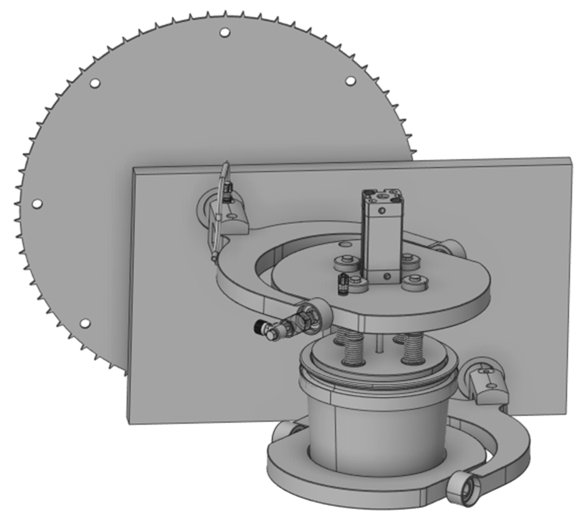
The mixing process of powder detergent is carried out in a 3D mixer, shown in Figure 1, that replicates the Turbula^® movement with a constant speed of 45 rpm. The components utilized to obtain the formulation are surfactant particles, sodium sulphate, sodium carbonate, coloured speckle, and liquid nonionic surfactant. Initially, every component is poured into the cup individually, except surfactant particles and liquid nonionic that are premixed before being poured. The cup has a capacity of 565 mL, and it was defined as having a filling grade of 70%. The properties of formulation components are shown in

Table 1. Properties of formulation components.

Component	Particle Size Median (µm)	Bulk Density (kg/m3)
Surfactant Particle	443	830
Sodium Sulphate	207	1550
Sodium Carbonate	655	1150
Coloured Speckle	1000	800
Liquid Nonionic Surfactant	-	800 1

¹ Density of the liquid component.

.

The mixing process has been modelled by the DEM method, which is typically used to study the behaviour of individual particles when interacting with each other and boundaries. The particle’s motion is governed by the equation of motion and the contact forces that act on them due to the interactions that occur with other particles and boundaries [6,16]. These contact forces consist of normal force and tangential force, and they are calculated according to the contact model used in the DEM simulation. In this work, the hysteretic linear spring model was selected to calculate the normal force, the linear spring coulomb limit to calculate the tangential force, and a constant adhesive force model to take into account the adhesion due to liquid bridge forces. The gravity action was also taken into account. Rocky DEM 4.4.3 software was used to perform the computational simulation.

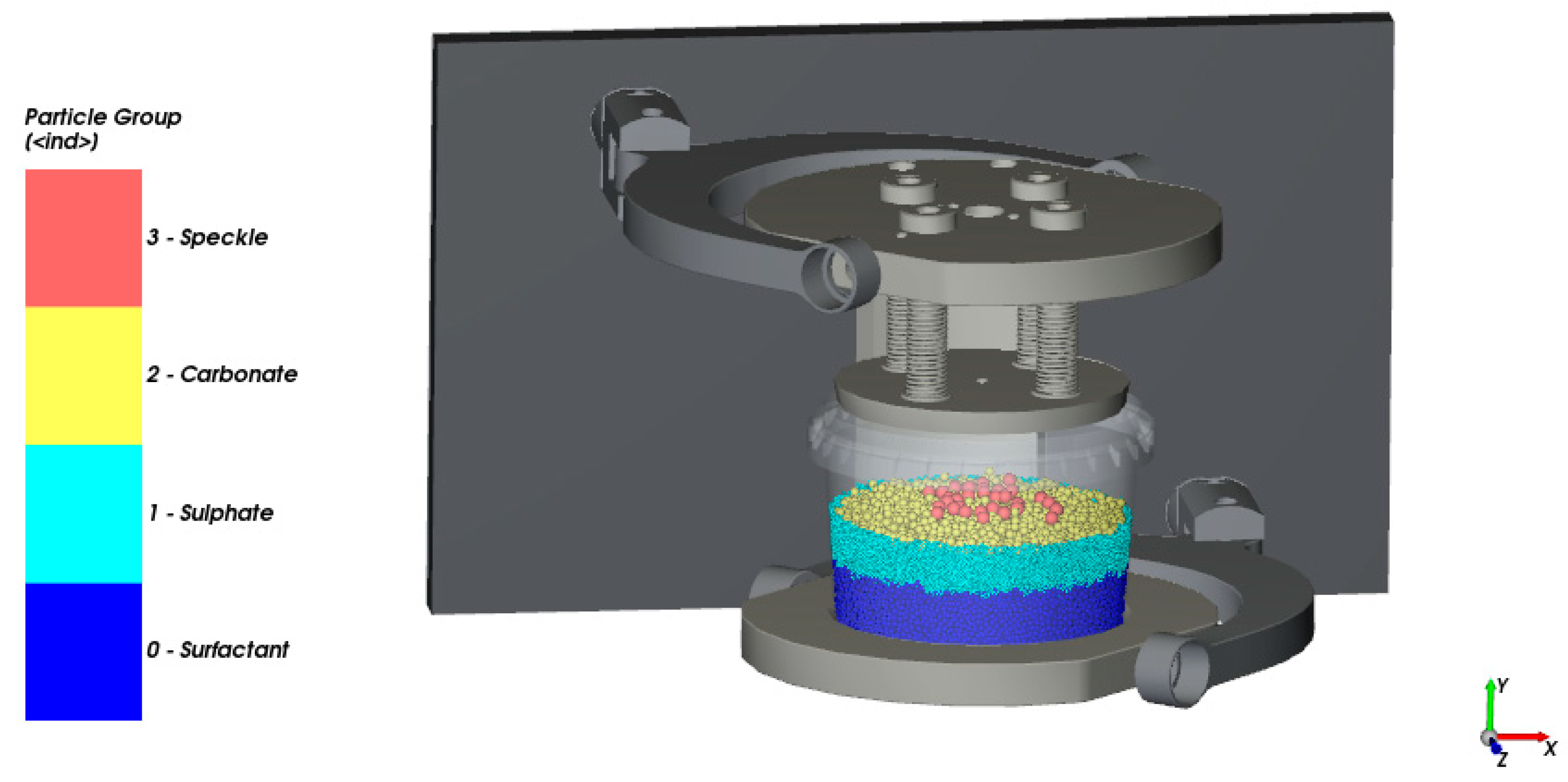
From the geometry of the 3D mixer, only the parts that affect the mixing process were included in the DEM model. To model the powder components, spherical particles were used, and the liquid component was modelled as a liquid film added to the particles, and the liquid amount added to each particle can change when particles interact between them. Due to the particle size of the different components, the modelling of the mixture was expected to generate a high number of particles with a high computational cost. Thus, the Same Statistic Weight (SSW) method has been considered, according to [17], by which a scale factor is applied to the particle size of all the components, achieving a reduction in the particle number to be modelled but keeping the initial shape of the particle size distribution.

Table 2. Input parameters for DEM model.

Component	Percentage by Mass (%)	Particle Size (mm)
Surfactant Particle	37.8	2.215
Sodium Sulphate	14.0	1.035
Sodium Carbonate	43.4	3.275
Coloured Speckle	0.7	5.0
Liquid Nonionic Surfactant	4.2	-

indicates the particle size of every component used in the DEM model, as well as the percentage by mass according to a standard formulation. The mechanical properties regarding interactions between particles, and between particles and boundaries, are presented in

Table 3. Mechanical properties from [18].

Parameter	Value
Particle–particle static friction	0.6
Particle–boundary static friction	0.4
Restitution coefficient	0.4
Rolling resistance	0.001

. The DEM model at the initial stage of the mixing process is shown in Figure 2, where a certain colour is assigned to every component. Initially, the powder components were totally segregated, and it was considered that the liquid component mass was equally distributed between particles of surfactant component.

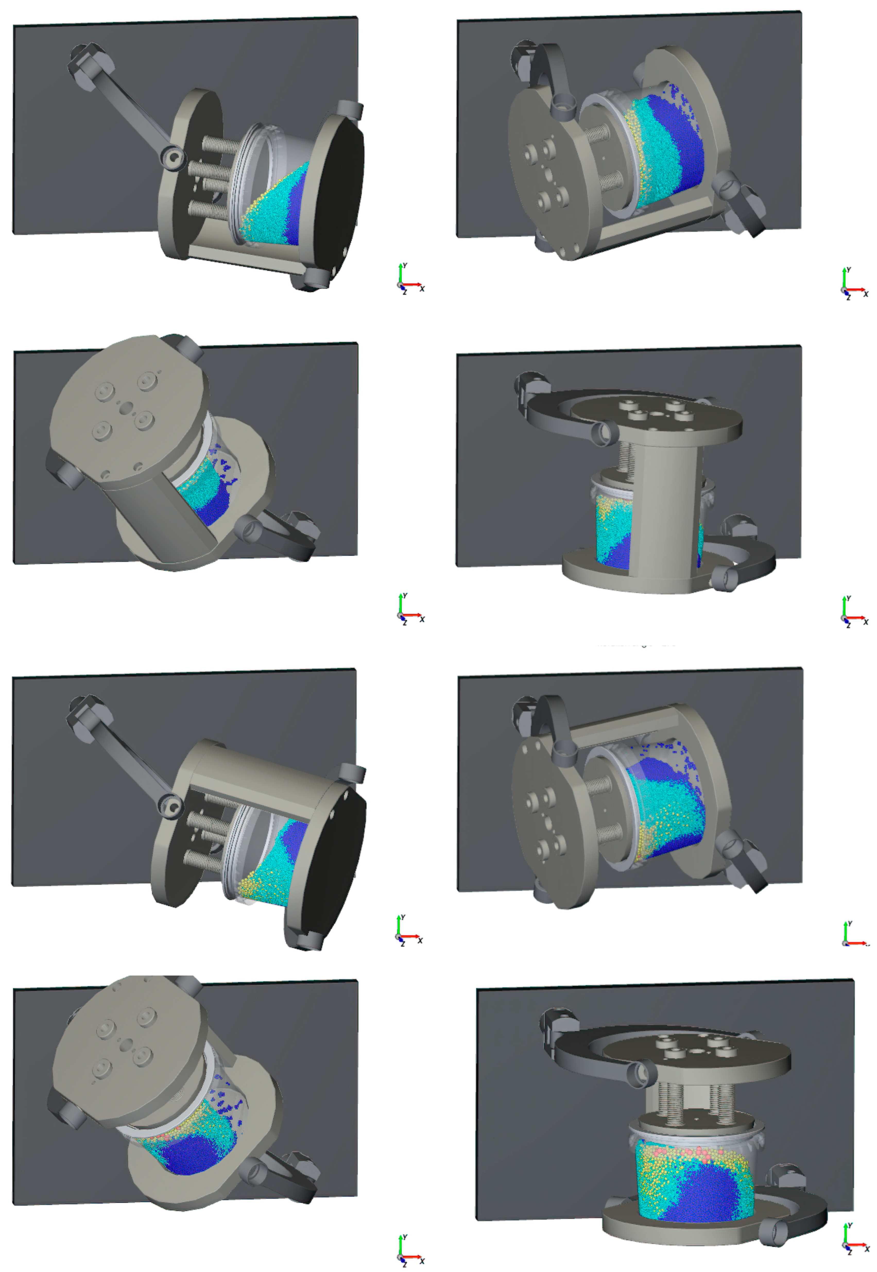
The Turbula^® movement is a three-dimensional movement based on the Schatz six-revolute mechanism [19], which has been employed to mixing powders. To replicate this movement, which was analysed in [20,21], an FEM model from the mixer geometry was created, and the parameterized position of every part during a cycle of movement was obtained by a rigid dynamics analysis. These position data were imported to the DEM software and applied to the DEM model. The movement described by the mixer model in each cycle is shown in Figure 3, representing the position of it every 45°.

Moreover, after introducing the mixing time, the DEM model simulates the mixing process up to the indicated time, and later it allows us to obtain the mixing performance of the process, defined as the output parameter, depending on the input parameters, which are time and components mass fraction.

In this study, the created DEM model was used to generate the dataset to estimate the mixing performance based on machine learning. This dataset contains a set of design points, where every point is defined by a certain value for every input parameter, and the corresponding value of the output parameter obtained from the DEM model.

To create the set of design points, the whole range of mass fraction of every component was considered. For that, a design of experiments (DOE) set was defined by the Central composite design (CCD), which is a five-level fractional factorial design that is suitable for calibrating quadratic response models. Using the CCD method, 25 design points were defined which are listed in

Table 4. DOE points. Percentage by mass (%) of input parameters.

Design Point	Surfactant Particle	Sodium Carbonate	Sodium Sulphate	Coloured Speckle	Liquid Nonionic Surfactant
1	25.0	0.9	72.1	1.0	1.0
2	25.0	0.9	68.7	1.0	4.4
3	25.0	0.9	73.1	0.0	1.0
4	25.0	0.9	69.7	0.0	4.4
5	25.0	36.7	36.3	1.0	1.0
6	25.0	36.7	32.9	1.0	4.4
7	25.0	36.7	37.3	0.0	1.0
8	25.0	36.7	33.9	0.0	4.4
9	40.0	0.9	57.1	1.0	1.0
10	40.0	0.9	53.7	1.0	4.4
11	40.0	0.9	58.1	0.0	1.0
12	40.0	0.9	54.7	0.0	4.4
13	40.0	36.7	21.3	1.0	1.0
14	40.0	36.7	17.9	1.0	4.4
15	40.0	36.7	22.3	0.0	1.0
16	40.0	36.7	18.9	0.0	4.4
17	32.5	18.8	45.5	0.5	2.7
18	25.0	18.8	53.0	0.5	2.7
19	40.0	18.8	38.0	0.5	2.7
20	32.5	0.9	63.4	0.5	2.7
21	32.5	36.7	27.6	0.5	2.7
22	32.5	18.8	46.0	0.0	2.7
23	32.5	18.8	45.0	1.0	2.7
24	32.5	18.8	47.2	0.5	1.0
25	32.5	18.8	43.8	0.5	4.4

.

3. Machine Learning Based Methodology

A machine learning (ML) algorithm based on multivariate polynomial regression (MPR) analysis was adopted to identify the relationship between variables and allowed the prediction of the mixing index.

The MPR used to estimate the coefficient values for different variables in the mixing process was derived from a Second Order Multiple Polynomial Regression expressed as:

$$y={\beta }_0+{\beta }_1{x}_1+{\beta }_2{x}_2+{\beta }_{11}{x}_1^2+{\beta }_{22}{x}_2^2+\epsilon$$

(1)

where β₁ and β₂ are called as linear effect parameters, β₁₁ and β₂₂ are called as quadratic effect parameters, β₀ is the bias, and ε is the error in the normal distribution.

According to [22], the Regression Function is given in Equation (2):

$$E\left(y\right)={\beta }_0+{\beta }_1{x}_1+{\beta }_2{x}_2+{\beta }_{11}{x}_1^2+{\beta }_{22}{x}_2^2$$

(2)

The representation of the polynomial regression in a matrix form is given in (3):

$$Y=\beta X+\epsilon$$

(3)

The estimated parameters can be computed as in Equation (4):

$$\widehat{\beta }={\left(X^{\prime }X\right)}^{-1}{X}^{\prime }Y$$

(4)

And the Computed Regression Equation is represented in (5):

$$\widehat{y}={\widehat{\beta }}_0+{\widehat{\beta }}_1{x}_1+{\widehat{\beta }}_2{x}_2+{\widehat{\beta }}_{11}{x}_1^2+{\widehat{\beta }}_{22}{x}_2^2$$

(5)

In order to assess the accuracy of the predicted values obtained by the regression-based ML model, the most used traditional metrics can be adopted [23]. MAPE (mean absolute percentage error), MAE (mean absolute error), RMSE (root mean square error), and R² (coefficient of determination) metrics were calculated as in Equations (6)–(9):

$$MAPE=\frac{100}{n}{\sum }_{i=1}^n\left|\frac{y_i-{\widehat{y}}_i}{y_i}\right|$$

(6)

$$MAE=\frac{1}{n}{\sum }_{i=1}^n\left|y_i-{\widehat{y}}_i\right|$$

(7)

$$RMSE=\sqrt{\frac{1}{n}{\sum }_{i=1}^n{\left(y_i-{\widehat{y}}_i\right)}^2}$$

(8)

$$R^2=1-\frac{{\sum }_{i=1}^n{\left(y_i-{\widehat{y}}_i\right)}^2}{{\sum }_{i=1}^n{\left(y_i-{\stackrel{-}{y}}_i\right)}^2};{\stackrel{-}{y}}_i=\frac{1}{n}{\sum }_{i=1}^n{y}_i$$

(9)

where y_i is the actual value, ${\widehat{y}}_i$ is the predicted value, and n is the number of data points.

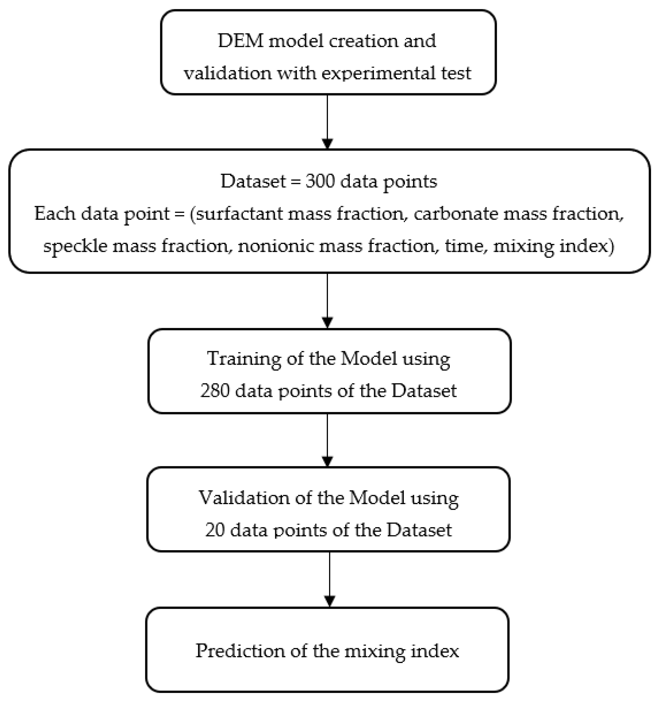
Figure 4 shows the flowchart of the methodology defined to predict the mixing index of the mixing process. The DEM model created is used to obtain the dataset. According the 25 design points listed in Table 4 and considering a time every 5 s from 5 to 60 s, a dataset of 300 data points was created. Each data point is composed by values of the inputs and the output. For the predictive model, the inputs are time and mass fraction of surfactant, carbonate, speckle and nonionic, and the output is the mixing index. The sulphate mass fraction is not considered an input because it depends on the total amount of the other components.

The dataset is divided into 2 parts. A total of 280 data points are used to train and test the predictive model. The other 20 data points are used to perform an independent validation of the model. In this process of training and validation, the accuracy of the predictive model results is assessed by calculating the error metrics indicated in Equations (6)–(9). Finally, the predictive model is obtained and allows us to predict the mixing index for any allowable combination of the components.

4. Results

The results show the validation of the DEM model compared with experimental results from a mixing test. In addition, the study of the effect of the initial component mass fraction and mixing time on the mixing performance is presented. The dataset acquired from this study was used to obtain a predictive model of the mixing index of the process that is also presented.

4.1. DEM Model Validation

To validate the DEM model, a mixing test with a 3D mixer was carried out and the mixture obtained from the test was used to determine the repose angle. The same procedure was simulated by the DEM model, and the numerical results were compared with the experimental ones. From a qualitative point of view, the mixing homogeneity was compared, and from a quantitative point of view, the repose angle.

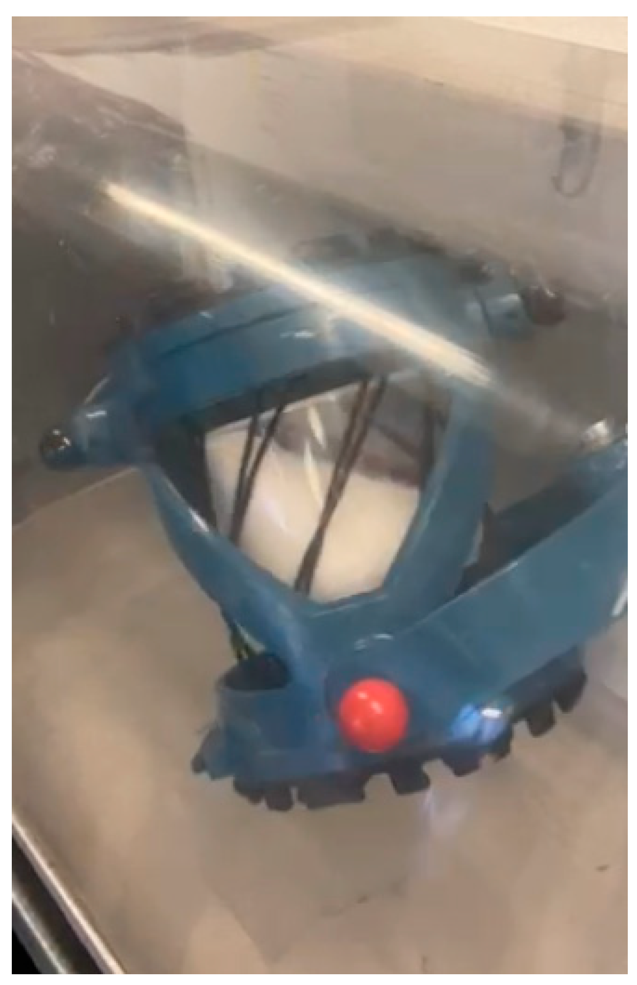
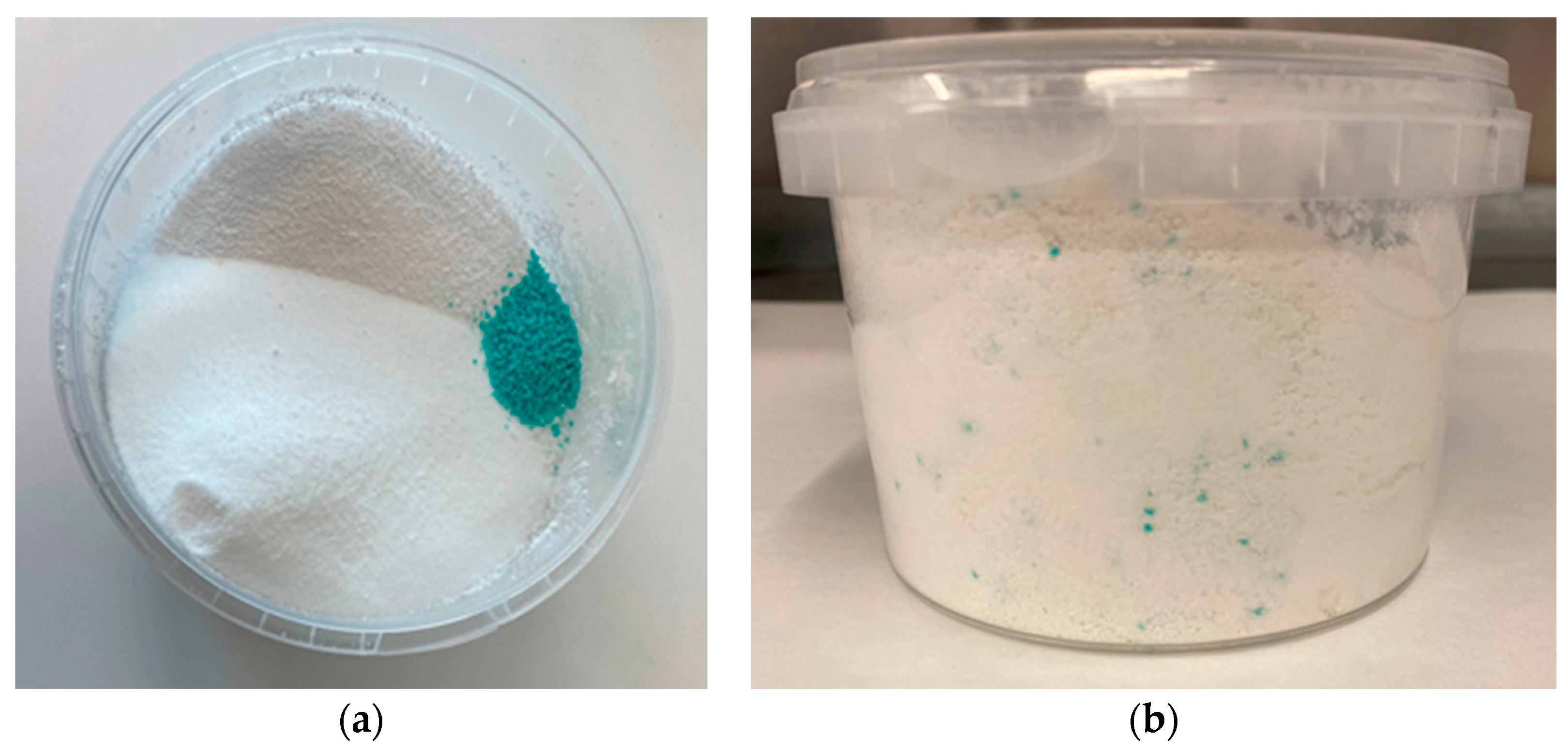
The methodology consisted of filling the cup with the component mass fraction according to the formulation shown in Table 2, closing the cup with a lid, placing it in a 3D mixer and running for 60 s. In Figure 5 a screenshot taken during the mixing test is observed. Figure 6 shows the cup filled with the components totally segregated before the test, and the cup with the components mixed after the test.

Once the mixing process was finished, a sample from the mixture was taken to determine the repose angle by the fixed funnel method according to [24]. Figure 7 presents a comparison between the powder piles obtained from test and DEM simulation. From a visual perspective, it is observed that a high grade of mixing has been obtained in both cases. The repose angle test was repeated twice and both times the result was 32°, while a repose angle of 31.98° was obtained from the DEM simulation, as indicated in

Table 5. Comparison of repose angle between numerical simulation and experimental test.

Repose Angle	Value
Numerical simulation	31.98°
Experimental test	32.00°
Relative error	0.063%

. Therefore, a great agreement between results from the experimental test and DEM simulation is observed.

4.2. Mixing Performance Analysis

After validating the DEM model with experimental results, it was used to analyse the mixing quality as a function of mass fraction components and mixing time. To assess the homogeneity of the powder multicomponent mixture, a mixing index based on the pooled variance of the whole system according to the study developed in [25] was used, whose criteria is expressed in the following equation:

$$M=\frac{{\sigma }_0^2-{\sigma }^2}{{\sigma }_0^2-{\sigma }_r^2}$$

(10)

where M is the mixing index, ${\sigma }^2$ is the unbiased sample variance of the concentration in a multicomponent mixture, ${\sigma }_r^2$ is the variance for multicomponent mixtures in the completely mixed state, and ${\sigma }_0^2$ is the variance for multicomponent mixtures in the completely segregated state. All these variances are calculated by DEM simulation for a defined input dataset. The M index can take values between 0, completely segregated, and 1, completely mixed.

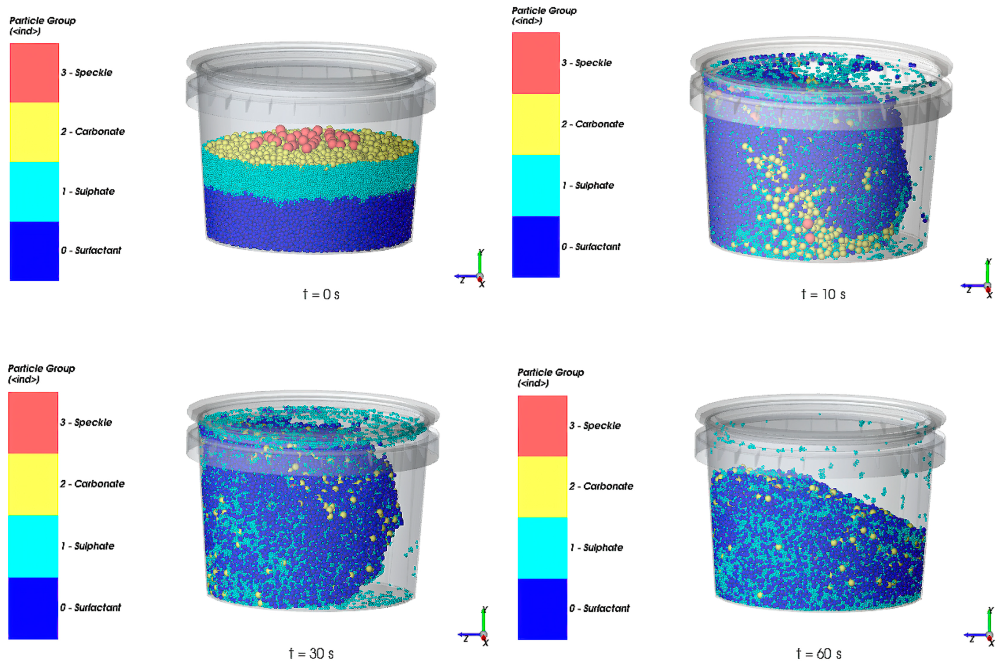
Every design point was simulated using the DEM model for a total mixing time of 60 s. The evolution of the mixture in the cup from the initial to the final instant of the process for the first design point is shown in Figure 8, where each represented instant matches with the end of a cycle of the mixer. A uniform mixing of particles is observed at 60 s from a visual point of view.

As time was defined as one of the input parameters, the M index output was obtained from DEM simulation every 5 s up to 60 s for all the design points, shown in

Table 6. M index output for each design point at t = 5, 10, 15, 20, 25, 30, 35, 40, 45, 50, 55, 60 s.

Design Point	Time (s)
	5	10	15	20	25	30	35	40	45	50	55	60
1	0.776	0.870	0.885	0.918	0.968	0.976	0.979	0.988	0.989	0.992	0.991	0.992
2	0.780	0.892	0.885	0.953	0.970	0.985	0.978	0.989	0.989	0.987	0.989	0.991
3	0.788	0.871	0.879	0.916	0.968	0.975	0.976	0.984	0.988	0.989	0.991	0.989
4	0.716	0.868	0.857	0.943	0.965	0.976	0.967	0.987	0.987	0.985	0.987	0.991
5	0.853	0.909	0.929	0.946	0.973	0.978	0.980	0.981	0.976	0.986	0.983	0.986
6	0.833	0.912	0.912	0.964	0.975	0.977	0.981	0.985	0.983	0.984	0.984	0.992
7	0.843	0.905	0.925	0.952	0.972	0.975	0.979	0.986	0.979	0.988	0.984	0.986
8	0.829	0.911	0.909	0.960	0.971	0.980	0.977	0.985	0.979	0.986	0.985	0.992
9	0.721	0.854	0.886	0.914	0.964	0.974	0.970	0.983	0.982	0.984	0.985	0.988
10	0.695	0.862	0.876	0.934	0.941	0.970	0.973	0.981	0.982	0.988	0.983	0.990
11	0.721	0.852	0.886	0.926	0.968	0.976	0.976	0.985	0.979	0.987	0.988	0.987
12	0.684	0.853	0.862	0.936	0.950	0.972	0.970	0.986	0.984	0.984	0.983	0.989
13	0.742	0.855	0.899	0.935	0.964	0.970	0.964	0.979	0.974	0.988	0.986	0.990
14	0.684	0.853	0.862	0.936	0.950	0.972	0.970	0.986	0.984	0.984	0.983	0.989
15	0.750	0.847	0.895	0.926	0.969	0.971	0.963	0.981	0.969	0.986	0.985	0.989
16	0.705	0.845	0.870	0.928	0.957	0.964	0.971	0.977	0.978	0.987	0.988	0.994
17	0.785	0.897	0.906	0.940	0.966	0.975	0.979	0.983	0.987	0.984	0.983	0.989
18	0.794	0.907	0.908	0.951	0.972	0.982	0.980	0.985	0.987	0.986	0.985	0.987
19	0.762	0.887	0.898	0.941	0.971	0.970	0.976	0.979	0.983	0.985	0.986	0.990
20	0.727	0.868	0.895	0.933	0.955	0.974	0.981	0.984	0.990	0.987	0.988	0.988
21	0.798	0.884	0.894	0.941	0.970	0.974	0.980	0.983	0.981	0.987	0.991	0.991
22	0.798	0.884	0.894	0.941	0.970	0.974	0.980	0.983	0.981	0.987	0.991	0.991
23	0.836	0.893	0.912	0.949	0.971	0.976	0.980	0.982	0.987	0.984	0.985	0.988
24	0.799	0.893	0.914	0.935	0.968	0.974	0.976	0.983	0.982	0.985	0.985	0.988
25	0.783	0.892	0.902	0.954	0.965	0.977	0.973	0.986	0.984	0.986	0.985	0.991

.

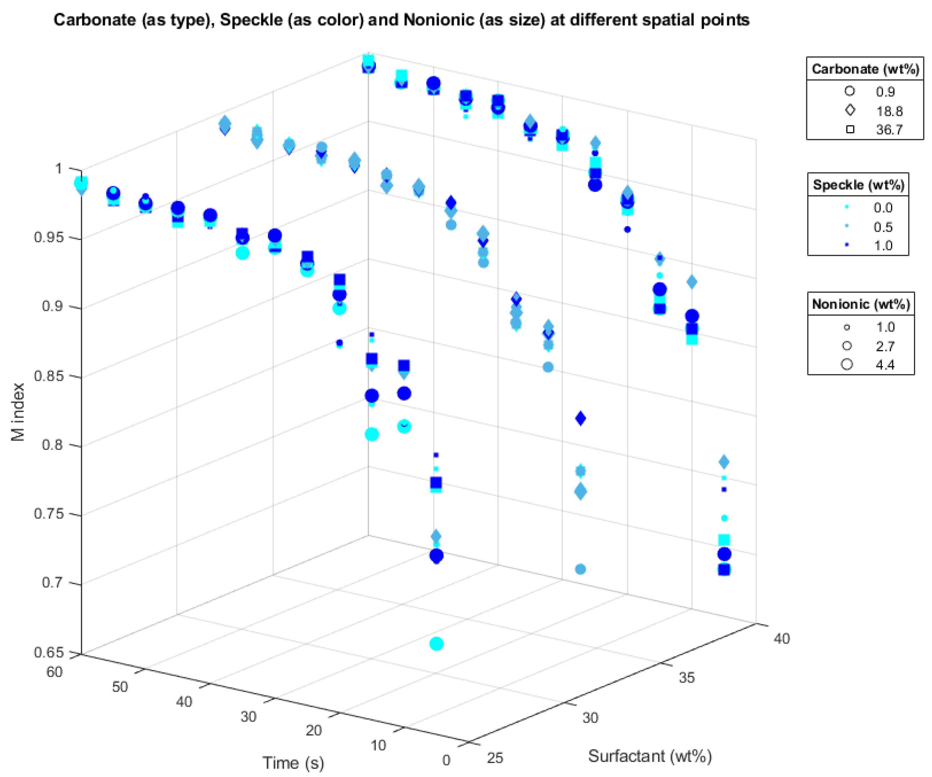
Figure 9 shows the variation of the M index with respect to time and the component mass fraction of surfactant, carbonate, speckle, and nonionic, where it was observed that the value of M index increases with time until it stabilizes at a value close to 1 in all cases analysed.

4.3. Predictive Model

The dataset of the powder mixing process obtained by the DEM model considering a defined range of every input variable, which are time and mass fraction of surfactant particles, sodium sulphate, sodium carbonate, coloured speckle, and liquid nonionic surfactant, was used to obtain a model that predicts the M index quickly and accurately from certain input values included in the ranges defined for them. For this purpose, a multivariate polynomial regression algorithm was used, which was trained and tested with 280 data points. After that, we validated the achieved model by means of an independent test dataset with 20 data points not used for training. The obtained model consists of the vector of coefficients used in the mathematical function, and is expressed in the following equation:

$$\begin{gathered} M=0.79399–0.18742x_{surfactant}+0.09510x_{carbonate}+0.54466x_{speckle}+ \\ 0.20182x_{nonionic}+0.01063x_{time}+0.15038x_{surfactant}^2-0.19728x_{carbonate}^2- \\ 28.44069x_{speckle}^2-4.90740x_{nonionic}^2-0.00012x_{time}^2 \end{gathered}$$

(11)

where M is the mixing index, x_surfactant is the mass fraction of surfactant particle, x_carbonate is the mass fraction of sodium carbonate, x_sulphate is the mass fraction of sodium sulphate, x_speckle is the mass fraction of coloured speckle, x_nonionic is the mass fraction of liquid nonionic surfactant, and x_time is the time in seconds.

The error metrics obtained to evaluate the training and validation of the model are presented in

Table 7. Error metrics.

Metric	MAPE (%)	MAE	RMSE	R2
Training	1.873	0.017	0.024	0.848
Validation	1.503	0.014	0.017	0.9072

.

5. Conclusions

In this work, the mixing process carried out by a 3D mixer for manufacturing a powder detergent was simulated using a DEM model, which was validated with experimental test. This computational model was used to study the mixing performance of the process considering mixing time and allowable mass fraction of components, at a mixer speed of 45 rpm. It was observed that a mixing index close to 1 was obtained in less than 60 s for all the combinations simulated, meaning that they were all completely mixed.

In addition, the proposed methodology based on DEM and ML to obtain a model which predicts the mixing index of the mixing process was developed. The DEM model was used to generate the dataset needed and a polynomial regression algorithm was used to obtain the model. It was demonstrated that the model predicts the mixing index of any allowable formulation with accuracy and in advance without requiring experimental test or numerical simulation. This method can also be used to optimize the mixing time necessary to obtain a uniform mixing of a defined formulation.

References

- Donzé, F.V.; Bouchez, J.; Magnier, S.A. Modeling fractures in rock blasting. Int. J. Rock Mech. Min. Sci. 1997, 34, 1153–1163. [Google Scholar] [CrossRef]
- Zhao, H.; Huang, Y.; Liu, Z.; Liu, W.; Zheng, Z. Applications of Discrete Element Method in the Research of Agricultural Machinery: A Review. Agriculture 2021, 11, 425. [Google Scholar] [CrossRef]
- Ghodki, M.; Goswami, T.K. DEM simulation of flow of black pepper seeds in cryogenic grinding system. J. Food Eng. 2017, 196, 36–51. [Google Scholar] [CrossRef]
- Ketterhagen, W.R.; Am Ende, M.T.; Hancock, B.C. Process Modeling in the Pharmaceutical Industry using the Discrete Element Method. J. Pharm. Sci. 2009, 98, 442–470. [Google Scholar] [CrossRef]
- Furukawa, R.; Shiosaka, Y.; Kadota, K.; Takagaki, K.; Noguchi, T.; Shimosaka, A.; Shirakawa, Y. Size-induced segregation during pharmaceutical particle die filling assessed by response surface methodology using discrete element method. J. Drug Deliv. Sci. Technol. 2016, 35, 284–293. [Google Scholar] [CrossRef]
- Bhalode, P.; Ierapetritou, M. Discrete element modeling for continuous powder feeding operation: Calibration and system analysis. Int. J. Pharm. 2020, 585, 119427. [Google Scholar] [CrossRef]
- Mayer-Laigle, C.; Gatumel, C.; Berthiaux, H. Mixing dynamics for easy flowing powders in a lab scale Turbula® mixer. Chem. Eng. Res. Des. 2015, 95, 248–261. [Google Scholar] [CrossRef]
- Harish, V.V.N.; Cho, M.; Shim, J. Effect of Rotating Cylinder on Mixing Performance in a Cylindrical Double-Ribbon Mixer. Appl. Sci. 2019, 9, 5179. [Google Scholar] [CrossRef]
- Marigo, M.; Cairns, D.L.; Davies, M.; Ingram, A.; Stitt, E.H. A numerical comparison of mixing efficiencies of solids in a cylindrical vessel subject to a range of motions. Powder Technol. 2012, 217, 540–547. [Google Scholar] [CrossRef]
- Zuo, Z.; Gong, S.; Xie, G.; Zhang, J. Sensitivity analysis of process parameters for granular mixing in an intensive mixer using response surface methodology. Powder Technol. 2021, 384, 51–61. [Google Scholar] [CrossRef]
- Sakai, M.; Shigeto, Y.; Basinskas, G.; Hosokawa, A.; Fuji, M. Discrete element simulation for the evaluation of solid mixing in an industrial blender. J. Chem. Eng. 2015, 279, 821–839. [Google Scholar] [CrossRef]
- Zhao, L.; Gu, H.; Ye, M.; Wei, M.; Xu, S.; Zuo, X. Optimization of the coupling parameters and mixing uniformity of multiple organic hydraulic mixtures based on the discrete element method and response surface methodology. Adv. Powder Technol. 2020, 31, 4365–4375. [Google Scholar] [CrossRef]
- Nguyen, V.T.T.; Dang, V.A.; Tran, N.T.; Nguyen, C.H.; Vo, D.H.; Nguyen, D.K.; Nguyen, N.L.; Nguyen, Q.L.; Tieu, T.L.; Bui, T.N.; et al. An investigation on design innovation, fabrication and experiment of a soy bean peeling machine-scale. Int. J. Eng. Technol. 2018, 7, 2704–2709. [Google Scholar] [CrossRef]
- Wang, C.; Yang, F.; Vo, N.T.; Nguyen, V.T.T. Wireless Communications for Data Security: Efficiency Assessment of Cybersecurity Industry—A Promising Application for UAVs. Drones 2022, 6, 363. [Google Scholar] [CrossRef]
- Kačur, J.; Flegner, P.; Durdán, M.; Laciak, M. Prediction of Temperature and Carbon Concentration in Oxygen Steelmaking by Machine Learning: A Comparative Study. Appl. Sci. 2022, 12, 7757. [Google Scholar] [CrossRef]
- ESSS Rocky DEM 2022. Available online: https://rocky.esss.co/software/ (accessed on 17 February 2023).
- Lu, L.; Xu, Y.; Li, T.; Benyahia, S. Assessment of different coarse graining strategies to simulate polydisperse gas-solids flow. Chem. Eng. Sci. 2018, 179, 53–63. [Google Scholar] [CrossRef]
- Thakur, S.C.; Ahmadian, H.; Sun, J.; Ooi, J.Y. An experimental and numerical study of packing, compression, and caking behaviour of detergent powders. Particuology 2014, 12, 2–12. [Google Scholar] [CrossRef]
- Lee, C. Analysis and Synthesis of Schatz Six-Revolute Mechanisms. JSME Int. J. C-Mech. Sy. 2000, 43, 80–91. [Google Scholar] [CrossRef]
- Marigo, M.; Davies, M.; Leadbeater, T.; Cairns, D.L.; Ingram, A.; Stitt, E.H. Application of Positron Emission Particle Tracking (PEPT) to validate a Discrete Element Method (DEM) model of granular flow and mixing in the Turbula mixer. Int. J. Pharm. 2013, 446, 46–58. [Google Scholar] [CrossRef]
- Marigo, M.; Cairns, D.; Davies, M.; Cook, M.; Ingram, A.; Stitt, E. Developing mechanistic understanding of granular behaviour in complex moving geometry using the discrete element method. Part A: Measurement and reconstruction of turbula® mixer motion using positron emission particle tracking. Comput. Model. Eng. Sci. 2010, 59, 217–238. [Google Scholar]
- Sinha, P. Multivariate polynomial regression in Data Mining: Methodology, problems and solutions. Int. J. Sci. Eng. Res. 2013, 4, 962–965. [Google Scholar]
- Naser, M.Z.; Alavi, A.H. Error Metrics and Performance Fitness Indicators for Artificial Intelligence and Machine Learning in Engineering and Sciences. Archit. Struct. Constr. 2021. [Google Scholar] [CrossRef]
- Al-Hashemi, H.M.B.; Al-Amoudi, O.S.B. A review on the angle of repose of granular materials. Powder Technol. 2018, 330, 397–417. [Google Scholar] [CrossRef]
- Fan, L.T.; Too, J.R.; Rubison, R.M.; Lai, F.S. Studies on multicomponent solids mixing and mixtures Part III. Mixing indices. Powder Technol. 1979, 24, 73–89. [Google Scholar] [CrossRef]
Figure 1.
Geometry of the mixer.
Figure 2.
DEM model of the mixing process.
Figure 3.
Replication of a cycle of the mixer. Screenshots every 45°.
Figure 4.
Flowchart of the methodology.
Figure 5.
Image of the mixing test performed in a 3D mixer.
Figure 6.
Mixing test. (a) Initial filling of the components in the cup; (b) mixture of the components after the mixing process.
Figure 7.
Powder pile from (a) experimental test and (b) DEM model.
Figure 8.
Simulation of design point 1 at different instants.
Figure 9.
A 6D scatter plot of the M index depending on the inputs surfactant, carbonate, speckle, nonionic and time.